Feasibility of Radar Vital Sign Monitoring Using Multiple Range Bin Selection

 , , , , and
Abstract
1. Introduction
2. Materials and Methods
2.1. FMCW Radar Measurement Principle
2.2. Chirp Median
2.3. Proposed Method
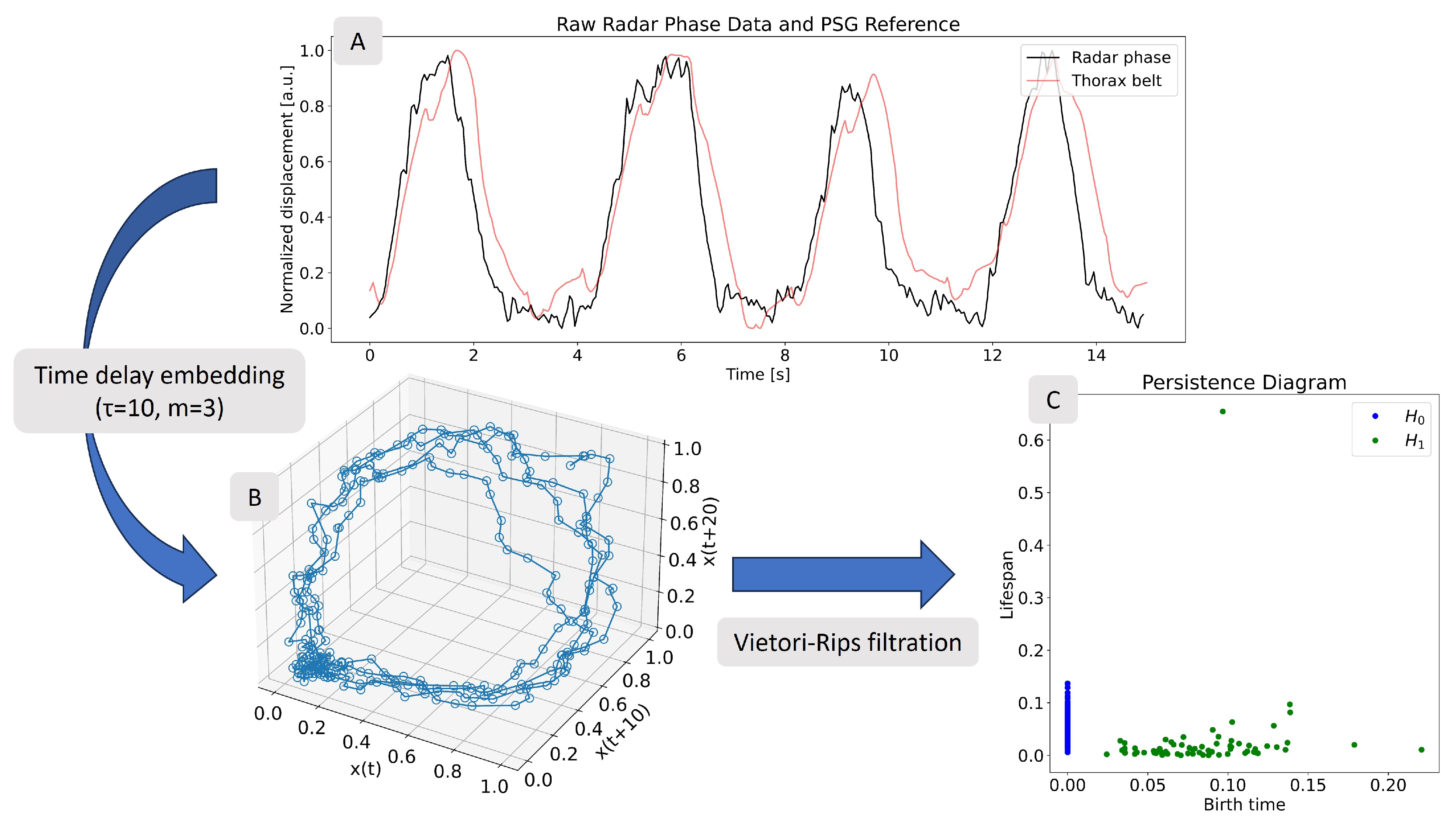
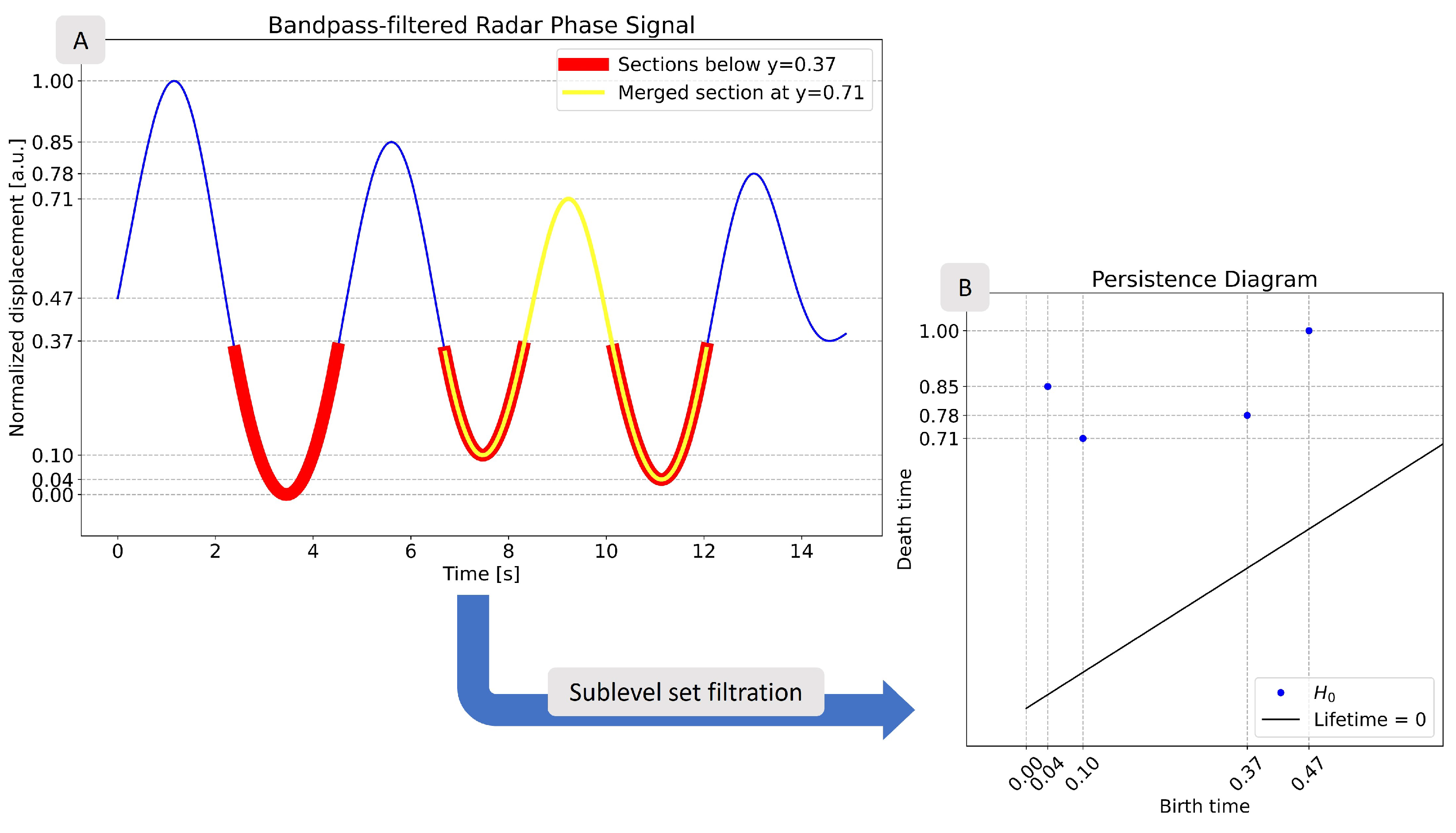
2.3.1. Methodology Background
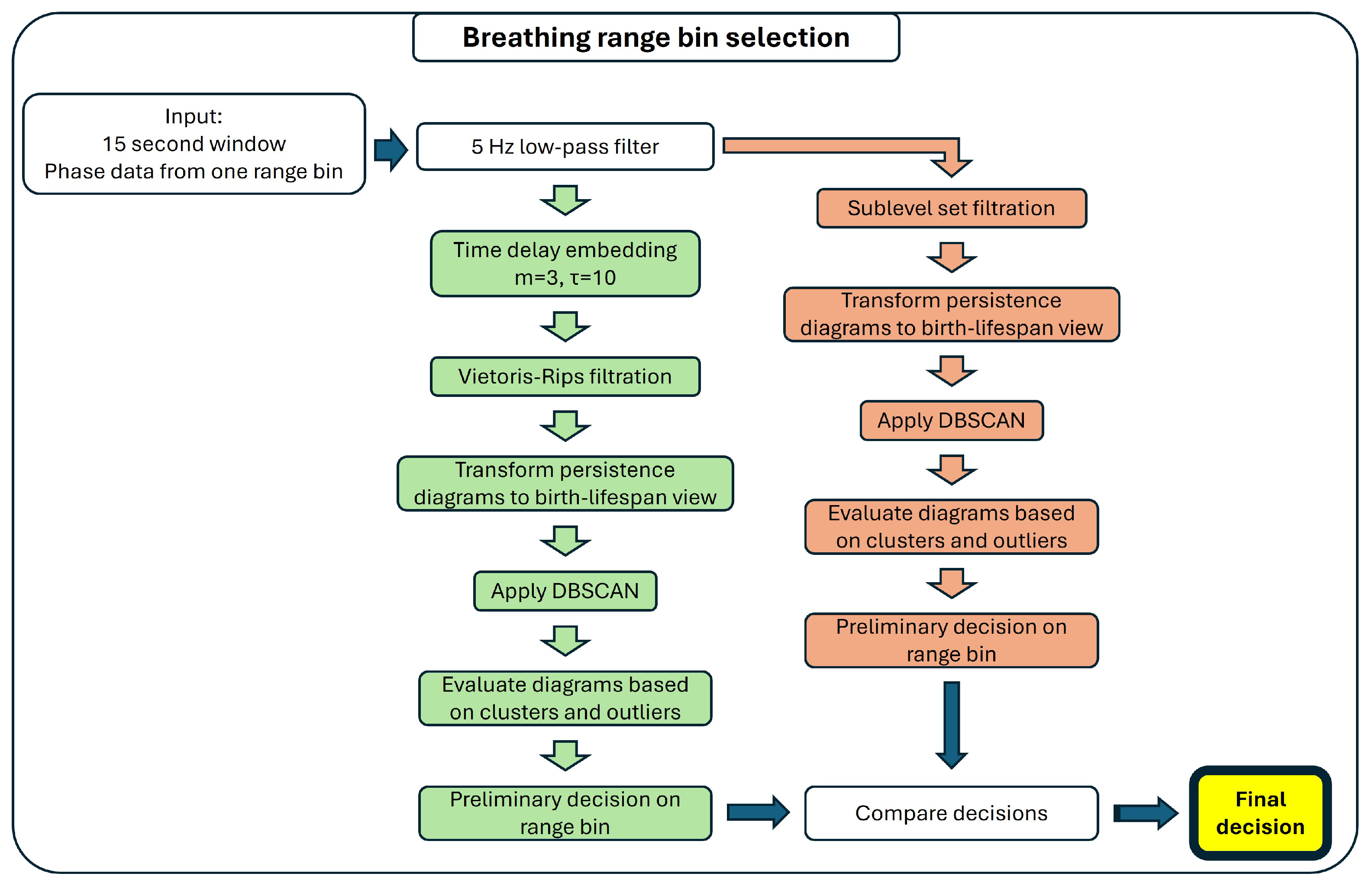
2.3.2. Multiple Range Bin Selection Method
Detection of Breathing
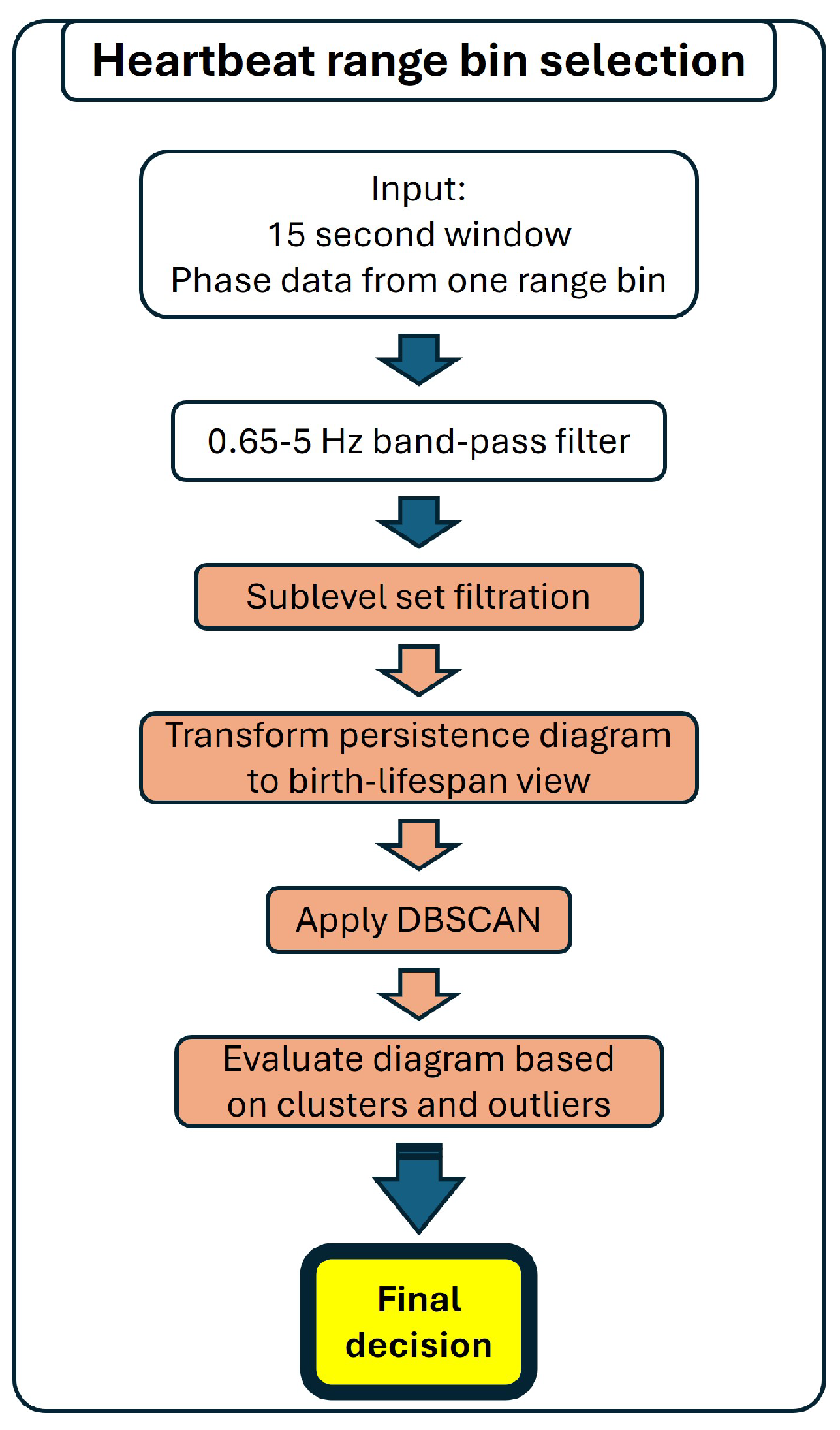
Detection of Heartbeat
2.4. Exploration of Windows with No Selected Range Bins
2.5. Vital Rate Computation
2.6. Description of Dataset
2.6.1. Study Description
2.6.2. Radar Device
2.6.3. Reference Device
2.6.4. Participants
2.7. Epoching and Range Bins of Interest
2.8. Dataset Size and Algorithm Run Time
2.9. Comparison with Single Bin Selection
3. Results
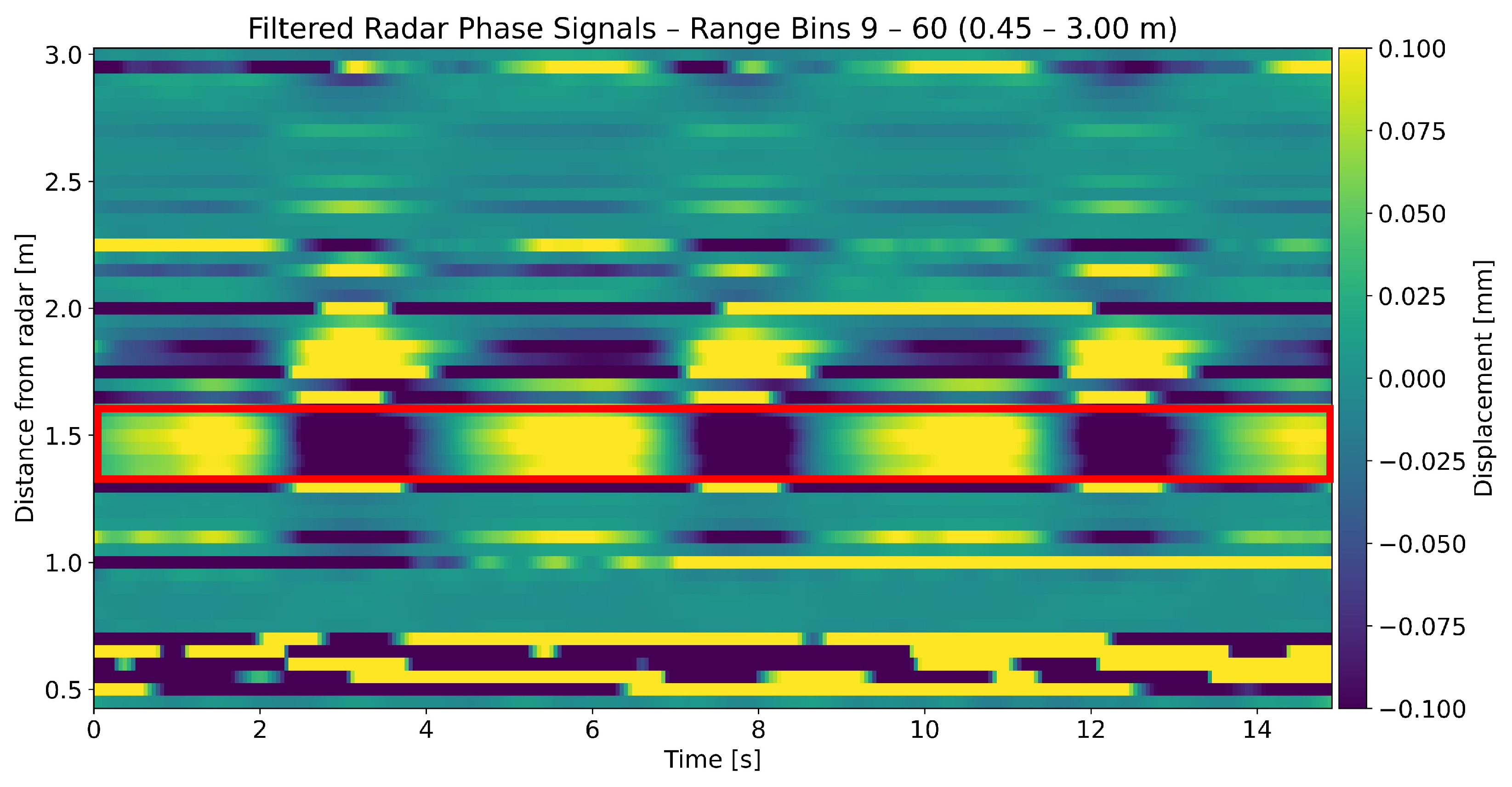
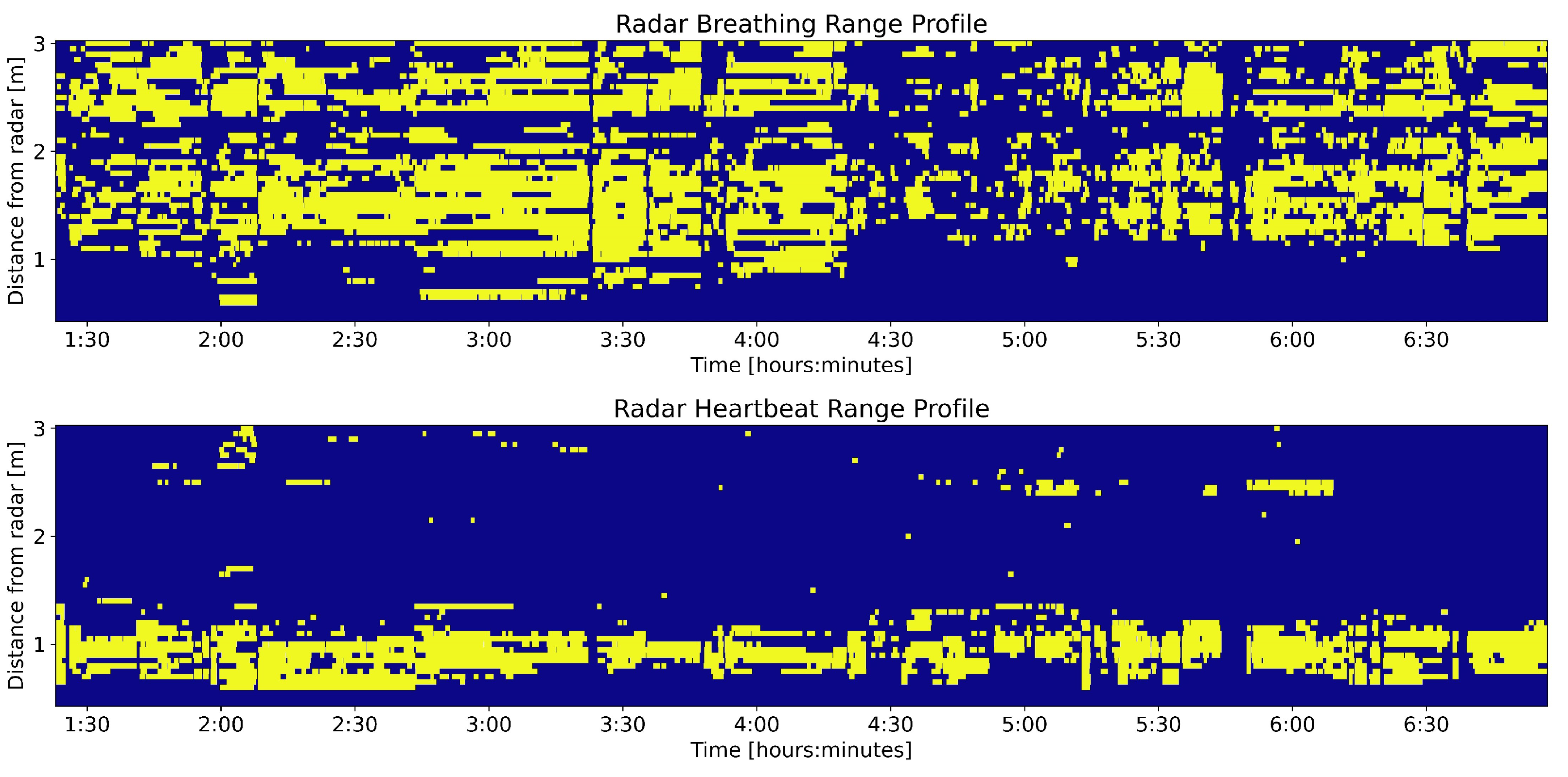
3.1. Range Profile
3.2. Exploration of Windows with No Selected Range Bins
3.3. Vital Rate Computation
3.3.1. Breathing Rate
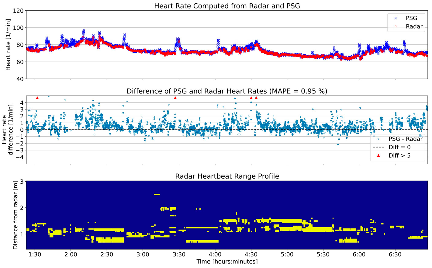
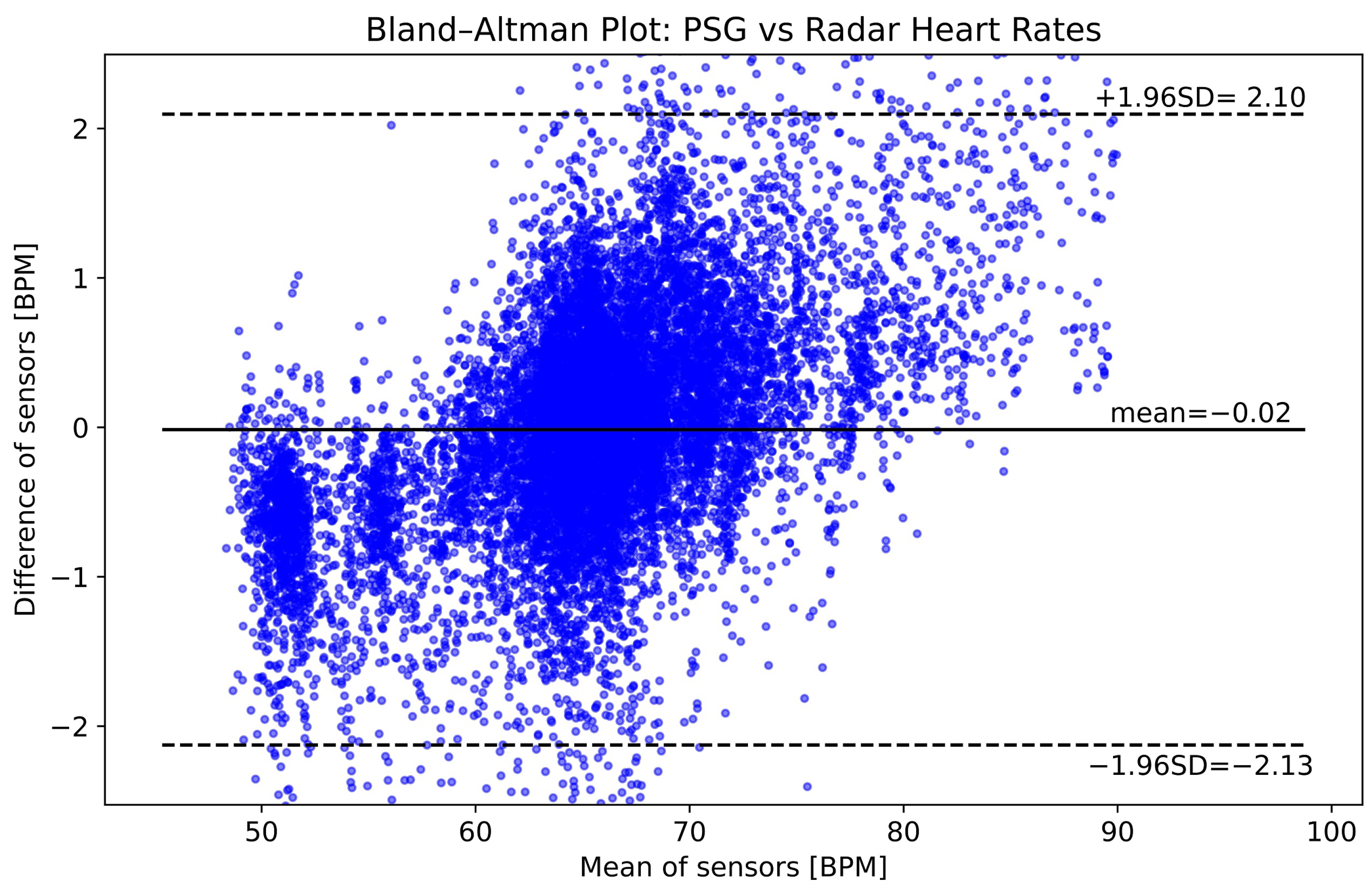
3.3.2. Heart Rate
4. Discussion
4.1. Interpretation of Results
4.2. Potential Uses of Range Profile
4.3. Limitations and Outlook
5. Conclusions
Author Contributions
Funding
Institutional Review Board Statement
Informed Consent Statement
Data Availability Statement
Acknowledgments
Conflicts of Interest
Abbreviations
| PSG | Polysomnography |
| EEG | Electroencephalogram |
| EOG | Electrooculogram |
| ECG | Electrocardiogram |
| EMG | Electromyogram |
| HST | Home Sleep Test |
| CW | Continuous Wave |
| FMCW | Frequency Modulated Continuous Wave |
| IR-UWB | Impulse Radio Ultra Wideband |
| TDA | Topological Data Analysis |
| IF | Intermediate Frequency |
| FFT | Fast Fourier Transform |
| TDE | Time Delay Embedding |
| BPM | Breaths/Beats per Minute |
| DBSCAN | Density-Based Spatial Clustering of Applications with Noise |
| SWT | Stationary Wavelet Transform |
| LSL | Lab Streaming Layer |
| MAE | Mean Absolute Error |
| MAPE | Mean Absolute Percent Error |
| OSAS | Obstructive Sleep Apnea Syndrome |
| COPD | Chronic Obstructive Pulmonary Disease |
References
- Lloyd-Jones, D.M.; Allen, N.B.; Anderson, C.A.; Black, T.; Brewer, L.C.; Foraker, R.E.; Grandner, M.A.; Lavretsky, H.; Perak, A.M.; Sharma, G.; et al. Life’s essential 8: Updating and enhancing the American Heart Association’s construct of cardiovascular health: A presidential advisory from the American Heart Association. Circulation 2022, 146, e18–e43. [Google Scholar] [CrossRef]
- Luyster, F.S.; Strollo, P.J., Jr.; Zee, P.C.; Walsh, J.K. Sleep: A health imperative. Sleep 2012, 35, 727–734. [Google Scholar] [CrossRef] [PubMed]
- Perry, G.S.; Patil, S.P.; Presley-Cantrell, L.R. Raising awareness of sleep as a healthy behavior. Prev. Chronic Dis. 2013, 10, E133. [Google Scholar] [CrossRef]
- Depner, C.M.; Stothard, E.R.; Wright, K.P. Metabolic consequences of sleep and circadian disorders. Curr. Diabetes Rep. 2014, 14, 1–9. [Google Scholar] [CrossRef] [PubMed]
- Liew, S.C.; Aung, T. Sleep deprivation and its association with diseases-a review. Sleep Med. 2021, 77, 192–204. [Google Scholar] [CrossRef] [PubMed]
- Inoue, Y.; Komada, Y. Sleep loss, sleep disorders and driving accidents. Sleep Biol. Rhythm. 2014, 12, 96–105. [Google Scholar] [CrossRef]
- Leger, D.; Bayon, V.; Ohayon, M.M.; Philip, P.; Ement, P.; Metlaine, A.; Chennaoui, M.; Faraut, B. Insomnia and accidents: Cross-sectional study (EQUINOX) on sleep-related home, work and car accidents in 5293 subjects with insomnia from 10 countries. J. Sleep Res. 2014, 23, 143–152. [Google Scholar] [CrossRef]
- Rundo, J.V.; Downey III, R. Polysomnography. Handb. Clin. Neurol. 2019, 160, 381–392. [Google Scholar]
- Markun, L.; Sampat, A. Clinician-focused overview and developments in polysomnography. Curr. Sleep Med. Rep. 2020, 6, 309–321. [Google Scholar] [CrossRef]
- Berry, R.B.; Budhiraja, R.; Gottlieb, D.J.; Gozal, D.; Iber, C.; Kapur, V.K.; Marcus, C.L.; Mehra, R.; Parthasarathy, S.; Quan, S.F.; et al. Rules for scoring respiratory events in sleep: Update of the 2007 AASM manual for the scoring of sleep and associated events: Deliberations of the sleep apnea definitions task force of the American Academy of Sleep Medicine. J. Clin. Sleep Med. 2012, 8, 597–619. [Google Scholar] [CrossRef]
- Flemons, W.W.; Douglas, N.J.; Kuna, S.T.; Rodenstein, D.O.; Wheatley, J. Access to diagnosis and treatment of patients with suspected sleep apnea. Am. J. Respir. Crit. Care Med. 2004, 169, 668–672. [Google Scholar] [CrossRef]
- Kapur, V.K.; Auckley, D.H.; Chowdhuri, S.; Kuhlmann, D.C.; Mehra, R.; Ramar, K.; Harrod, C.G. Clinical practice guideline for diagnostic testing for adult obstructive sleep apnea: An American Academy of Sleep Medicine clinical practice guideline. J. Clin. Sleep Med. 2017, 13, 479–504. [Google Scholar] [CrossRef] [PubMed]
- Le Bon, O.; Staner, L.; Hoffmann, G.; Dramaix, M.; San Sebastian, I.; Murphy, J.R.; Kentos, M.; Pelc, I.; Linkowski, P. The first-night effect may last more than one night. J. Psychiatr. Res. 2001, 35, 165–172. [Google Scholar] [CrossRef] [PubMed]
- Ding, L.; Chen, B.; Dai, Y.; Li, Y. A meta-analysis of the first-night effect in healthy individuals for the full age spectrum. Sleep Med. 2022, 89, 159–165. [Google Scholar] [CrossRef]
- Kapoor, M.; Greenough, G. Home sleep tests for obstructive sleep apnea (OSA). J. Am. Board Fam. Med. 2015, 28, 504–509. [Google Scholar] [CrossRef]
- Yoon, H.; Choi, S.H. Technologies for sleep monitoring at home: Wearables and nearables. Biomed. Eng. Lett. 2023, 13, 313–327. [Google Scholar] [CrossRef] [PubMed]
- Penzel, T.; Fietze, I.; Glos, M. Alternative algorithms and devices in sleep apnoea diagnosis: What we know and what we expect. Curr. Opin. Pulm. Med. 2020, 26, 650–656. [Google Scholar] [CrossRef]
- Boiko, A.; Martínez Madrid, N.; Seepold, R. Contactless technologies, sensors, and systems for cardiac and respiratory measurement during sleep: A systematic review. Sensors 2023, 23, 5038. [Google Scholar] [CrossRef]
- Balali, P.; Rabineau, J.; Hossein, A.; Tordeur, C.; Debeir, O.; Van De Borne, P. Investigating cardiorespiratory interaction using ballistocardiography and seismocardiography—A narrative review. Sensors 2022, 22, 9565. [Google Scholar] [CrossRef]
- Dafna, E.; Tarasiuk, A.; Zigel, Y. Sleep staging using nocturnal sound analysis. Sci. Rep. 2018, 8, 13474. [Google Scholar] [CrossRef]
- van Meulen, F.B.; Grassi, A.; Van den Heuvel, L.; Overeem, S.; van Gilst, M.M.; van Dijk, J.P.; Maass, H.; Van Gastel, M.J.; Fonseca, P. Contactless camera-based sleep staging: The healthbed study. Bioengineering 2023, 10, 109. [Google Scholar] [CrossRef] [PubMed]
- Turppa, E.; Kortelainen, J.M.; Antropov, O.; Kiuru, T. Vital sign monitoring using FMCW radar in various sleeping scenarios. Sensors 2020, 20, 6505. [Google Scholar] [CrossRef] [PubMed]
- Liebetruth, M.; Kehe, K.; Steinritz, D.; Sammito, S. Systematic Literature Review Regarding Heart Rate and Respiratory Rate Measurement by Means of Radar Technology. Sensors 2024, 24, 1003. [Google Scholar] [CrossRef]
- Boric-Lubecke, O.; Lubecke, V.M.; Droitcour, A.D.; Park, B.K.; Singh, A. Doppler Radar Physiological Sensing; John Wiley & Sons: Hoboken, NJ, USA, 2015. [Google Scholar]
- Paterniani, G.; Sgreccia, D.; Davoli, A.; Guerzoni, G.; Di Viesti, P.; Valenti, A.C.; Vitolo, M.; Vitetta, G.M.; Boriani, G. Radar-based monitoring of vital signs: A tutorial overview. Proc. IEEE 2023, 111, 277–317. [Google Scholar] [CrossRef]
- Hong, H.; Zhang, L.; Gu, C.; Li, Y.; Zhou, G.; Zhu, X. Noncontact sleep stage estimation using a CW Doppler radar. IEEE J. Emerg. Sel. Top. Circuits Syst. 2018, 8, 260–270. [Google Scholar] [CrossRef]
- Choi, H.I.; Song, W.J.; Song, H.; Shin, H.C. Selecting target range with accurate vital sign using spatial phase coherency of FMCW radar. Appl. Sci. 2021, 11, 4514. [Google Scholar] [CrossRef]
- Choi, H.I.; Song, W.J.; Song, H.; Shin, H.C. Improved heartbeat detection by exploiting temporal phase coherency in FMCW radar. IEEE Access 2021, 9, 163654–163664. [Google Scholar] [CrossRef]
- Wang, G.; Gu, C.; Inoue, T.; Li, C. A hybrid FMCW-interferometry radar for indoor precise positioning and versatile life activity monitoring. IEEE Trans. Microw. Theory Tech. 2014, 62, 2812–2822. [Google Scholar] [CrossRef]
- Hornig, L.; Szmola, B.; Pätzold, W.; Vox, J.P.; Wolf, K.I. Evaluation of Lateral Radar Positioning for Vital Sign Monitoring: An Empirical Study. Sensors 2024, 24, 3548. [Google Scholar] [CrossRef]
- Khan, F.; Cho, S.H. A detailed algorithm for vital sign monitoring of a stationary/non-stationary human through IR-UWB radar. Sensors 2017, 17, 290. [Google Scholar] [CrossRef]
- Zomorodian, A.; Carlsson, G. Computing Persistent Homology. Discret. Comput. Geom. 2005, 33, 249–274. [Google Scholar] [CrossRef]
- Ravishanker, N.; Chen, R. An introduction to persistent homology for time series. Wiley Interdiscip. Rev. Comput. Stat. 2021, 13, e1548. [Google Scholar] [CrossRef]
- Chung, Y.M.; Huang, W.K.; Wu, H.T. Topological data analysis assisted automated sleep stage scoring using airflow signals. Biomed. Signal Process. Control 2024, 89, 105760. [Google Scholar] [CrossRef]
- Chung, Y.M.; Hu, C.S.; Lo, Y.L.; Wu, H.T. A persistent homology approach to heart rate variability analysis with an application to sleep-wake classification. Front. Physiol. 2021, 12, 637684. [Google Scholar] [CrossRef] [PubMed]
- Takens, F. Detecting strange attractors in turbulence. In Dynamical Systems and Turbulence, Warwick 1980: Proceedings of a Symposium Held at the University of Warwick 1979/80; Springer: Berlin/Heidelberg, Germany, 2006; pp. 366–381. [Google Scholar]
- Tan, E.; Algar, S.; Corrêa, D.; Small, M.; Stemler, T.; Walker, D. Selecting embedding delays: An overview of embedding techniques and a new method using persistent homology. Chaos Interdiscip. J. Nonlinear Sci. 2023, 33, 032101. [Google Scholar] [CrossRef]
- Skaf, Y.; Laubenbacher, R. Topological data analysis in biomedicine: A review. J. Biomed. Informatics 2022, 130, 104082. [Google Scholar] [CrossRef]
- Erden, F.; Cetin, A.E. Period estimation of an almost periodic signal using persistent homology with application to respiratory rate measurement. IEEE Signal Process. Lett. 2017, 24, 958–962. [Google Scholar] [CrossRef]
- Wang, Y.; Wang, W.; Zhou, M.; Ren, A.; Tian, Z. Remote monitoring of human vital signs based on 77-GHz mm-wave FMCW radar. Sensors 2020, 20, 2999. [Google Scholar] [CrossRef]
- Pauli, M.; Göttel, B.; Scherr, S.; Bhutani, A.; Ayhan, S.; Winkler, W.; Zwick, T. Miniaturized millimeter-wave radar sensor for high-accuracy applications. IEEE Trans. Microw. Theory Tech. 2017, 65, 1707–1715. [Google Scholar] [CrossRef]
- Piotrowsky, L.; Jaeschke, T.; Kueppers, S.; Siska, J.; Pohl, N. Enabling high accuracy distance measurements with FMCW radar sensors. IEEE Trans. Microw. Theory Tech. 2019, 67, 5360–5371. [Google Scholar] [CrossRef]
- Bhutani, A.; Marahrens, S.; Gehringer, M.; Göttel, B.; Pauli, M.; Zwick, T. The role of millimeter-waves in the distance measurement accuracy of an FMCW radar sensor. Sensors 2019, 19, 3938. [Google Scholar] [CrossRef]
- Cretikos, M.A.; Bellomo, R.; Hillman, K.; Chen, J.; Finfer, S.; Flabouris, A. Respiratory rate: The neglected vital sign. Med. J. Aust. 2008, 188, 657–659. [Google Scholar] [CrossRef] [PubMed]
- Hill, B.; Annesley, S.H. Monitoring respiratory rate in adults. Br. J. Nurs. 2020, 29, 12–16. [Google Scholar] [CrossRef]
- Mason, J.W.; Ramseth, D.J.; Chanter, D.O.; Moon, T.E.; Goodman, D.B.; Mendzelevski, B. Electrocardiographic reference ranges derived from 79,743 ambulatory subjects. J. Electrocardiol. 2007, 40, 228–234. [Google Scholar] [CrossRef]
- Avram, R.; Tison, G.H.; Aschbacher, K.; Kuhar, P.; Vittinghoff, E.; Butzner, M.; Runge, R.; Wu, N.; Pletcher, M.J.; Marcus, G.M.; et al. Real-world heart rate norms in the Health eHeart study. NPJ Digit. Med. 2019, 2, 58. [Google Scholar] [CrossRef] [PubMed]
- Tralie, C.; Saul, N.; Bar-On, R. Ripser.py: A Lean Persistent Homology Library for Python. J. Open Source Softw. 2018, 3, 925. [Google Scholar] [CrossRef]
- Ester, M.; Kriegel, H.P.; Sander, J.; Xu, X. A density-based algorithm for discovering clusters in large spatial databases with noise. In Proceedings of the Second International Conference on Knowledge Discovery and Data Mining, Portland, OR, USA, 2–4 August 1996; Volume 96, pp. 226–231. [Google Scholar]
- Lawson, A.; Hoffman, T.; Chung, Y.M.; Keegan, K.; Day, S. A density-based approach to feature detection in persistence diagrams for firn data. Found. Data Sci. 2022, 4, 623–639. [Google Scholar] [CrossRef]
- Kothe, C.A. Lab Streaming Layer. [Computer Software]. Version 1.15.0. Available online: https://github.com/sccn/labstreaminglayer (accessed on 10 January 2024).
- Farre, R.; Montserrat, J.; Navajas, D. Noninvasive monitoring of respiratory mechanics during sleep. Eur. Respir. J. 2004, 24, 1052–1060. [Google Scholar] [CrossRef]
- Cano Porras, D.; Lunardi, A.C.; Marques da Silva, C.C.; Paisani, D.M.; Stelmach, R.; Moriya, H.T.; Carvalho, C.R. Comparison between the phase angle and phase shift parameters to assess thoracoabdominal asynchrony in COPD patients. J. Appl. Physiol. 2017, 122, 1106–1113. [Google Scholar] [CrossRef]


| Time Windows Where at Least One Range Bin Was Selected for Breathing | Time Windows Where No Range Bins Were Selected for Breathing | |
|---|---|---|
| Standard deviation quartiles [V] | 170.06–240.93–329.88 | 650.44–879.18–1140.04 |
| Percentage of windows where abs. skewness > 1 [%] | 15.70 | 46.30 |
| Percentage of windows where abs. kurtosis > 3 [%] | 15.16 | 59.49 |
| Time Windows Where at Least One Range Bin Selected Was for Heartbeat | Time Windows Where No Range Bins Were Selected for Heartbeat | |
|---|---|---|
| Magnitude standard deviation quartiles [V] | 50.47–98.92–192.85 | 280.83–473.13–735.26 |
| Percentage of windows where abs. skewness > 1 [%] | 17.92 | 32.85 |
| Percentage of windows where abs. kurtosis > 3 [%] | 17.76 | 46.92 |
| Single Bin Selection [30] | Proposed Method with Chirp Median | Proposed Method Using 1st Chirp | |
|---|---|---|---|
| Windows where PSG rate was computed [% (count)] | 94 (5583) | 93.6 (22,563) | 93.6 (22,563) |
| Windows where radar rate was computed [% (count)] | 98.5 (5851) | 90 (21,680) | 89.8 (21,651) |
| Duration where no PSG rate was computed [hh:mm:ss] | 00:12:00 | 00:04:25 | 00:04:25 |
| Duration where no radar rate was computed [hh:mm:ss] | 00:05:00 | 00:50:15 | 00:52:15 |
| Windows where difference between PSG and radar < ± 1 BPM [% (count)] | 93.2 (5151) | 96.4 (20,182) | 96.4 (20,167) |
| Mean Absolute Error [1/min] | 0.29 | 0.20 | 0.20 |
| Mean Absolute Percent Error [%] | 2.24 | 1.48 | 1.50 |
| Single Bin Selection [30] | Proposed Method with Chirp Median | Proposed Method Using 1st Chirp | |
|---|---|---|---|
| Windows where PSG rate was computed [% (count)] | 92.6 (5503) | 92.4 (22,279) | 92.4 (22,279) |
| Windows where radar rate was computed [% (count)] | 70.6 (4194) | 59.7 (14,379) | 54.4 (13,101) |
| Duration where no PSG rate was computed [hh:mm:ss] | 01:48:00 | 01:41:00 | 01:41:00 |
| Duration where no radar rate was computed [hh:mm:ss] | 05:53:40 | 07:45:55 | 10:10:35 |
| Windows where difference between PSG and radar < ± 1 BPM [% (count)] | 58.2 (2332) | 81.6 (11,379) | 68.0 (8628) |
| Mean Absolute Error [1/min] | 1.97 | 0.66 | 0.93 |
| Mean Absolute Percent Error [%] | 3.25 | 1.02 | 1.39 |
Disclaimer/Publisher’s Note: The statements, opinions and data contained in all publications are solely those of the individual author(s) and contributor(s) and not of MDPI and/or the editor(s). MDPI and/or the editor(s) disclaim responsibility for any injury to people or property resulting from any ideas, methods, instructions or products referred to in the content. |
© 2025 by the authors. Licensee MDPI, Basel, Switzerland. This article is an open access article distributed under the terms and conditions of the Creative Commons Attribution (CC BY) license (https://creativecommons.org/licenses/by/4.0/).
Share and Cite
Szmola, B.; Hornig, L.; Wolf, K.I.; Radeloff, A.; Witt, K.; Kollmeier, B. Feasibility of Radar Vital Sign Monitoring Using Multiple Range Bin Selection. Sensors 2025, 25, 2596. https://doi.org/10.3390/s25082596
Szmola B, Hornig L, Wolf KI, Radeloff A, Witt K, Kollmeier B. Feasibility of Radar Vital Sign Monitoring Using Multiple Range Bin Selection. Sensors. 2025; 25(8):2596. https://doi.org/10.3390/s25082596
Chicago/Turabian StyleSzmola, Benedek, Lars Hornig, Karen Insa Wolf, Andreas Radeloff, Karsten Witt, and Birger Kollmeier. 2025. "Feasibility of Radar Vital Sign Monitoring Using Multiple Range Bin Selection" Sensors 25, no. 8: 2596. https://doi.org/10.3390/s25082596
APA StyleSzmola, B., Hornig, L., Wolf, K. I., Radeloff, A., Witt, K., & Kollmeier, B. (2025). Feasibility of Radar Vital Sign Monitoring Using Multiple Range Bin Selection. Sensors, 25(8), 2596. https://doi.org/10.3390/s25082596