Article

Photovoltaic System with a Battery-Assisted Quasi-Z-Source Inverter: Improved Control System Design Based on a Novel Small-Signal Model

Faculty of Electrical Engineering, Mechanical Engineering and Naval Architecture, Department of Power Engineering, University of Split, 21000 Split, Croatia
*
Author to whom correspondence should be addressed.
Energies 2022, 15(3), 850; https://doi.org/10.3390/en15030850
Submission received: 13 December 2021 / Revised: 14 January 2022 / Accepted: 21 January 2022 / Published: 24 January 2022
(This article belongs to the Special Issue Advanced Control Techniques for Wind/Solar/Battery Systems)

Abstract

:
This paper deals with a photovoltaic (PV) system containing a quasi-Z-source inverter (qZSI) and batteries connected in parallel with the qZSI’s lower-voltage capacitor. The control system design is based on knowledge of three transfer functions which are obtained from the novel small-signal model of the considered system. The transfer function from the d-axis grid current to the battery current has been identified for the first time in this study for the considered system configuration and has been utilized for the design of the battery current control loop for the grid-tied operation. The transfer function from the duty cycle to the PV source voltage has been utilized for the design of the PV source voltage control loop. The PV source voltage is controlled so as to ensure the desired power production of the PV source. For the maximum power point tracking, a perturb-and-observe algorithm is utilized that does not require the measurement of the PV source current, but it instead utilizes the battery current during the stand-alone operation and the d-axis reference current during the grid-tied operation. The corresponding tracking period was determined by using the transfer function from the duty cycle to the battery current and in accordance with the longest settling time noted in the corresponding step response. The proposed control algorithm also has integrated protection against battery overcharging during the stand-alone operation. The considered system has been experimentally tested over wide ranges of irradiance and PV panel temperature.

1. Introduction

Solar energy as a clean and fully renewable source of energy can be harnessed all over the world and directly converted to electricity by means of photovoltaic (PV) systems. The main component of these systems is a PV source composed of multiple interconnected PV panels. The PV source produces dc voltage and current, so in the case of the grid-tied operation or the stand-alone operation with ac loads, it is commonly combined with a dc–dc boost converter, to ensure required voltage boost and maximum power production of a PV source, and a voltage-source inverter [1,2,3]. The alternative is the utilization of a quasi-Z-source inverter (qZSI) [4], which enables both the boost and control of the PV source voltage, thus eliminating the requirement for a dc–dc converter. The qZSI ensures boost of the input voltage by means of an impedance network and the additional shoot-through (ST) switching state, which is achieved by short circuiting one or all of the inverter legs during the zero-switching states of the inverter.
The combination of the PV source and the qZSI has been in the scope of many recent studies. In [5,6], PV systems containing the qZSI in the grid-tied applications are analyzed, where the main tasks of the corresponding control algorithms are to ensure the maximum power production of the PV source and injection of that power into the grid. The main disadvantage of the mentioned systems is the absence of an energy-storage system, so during the stand-alone operation the PV source power has to be equal to the sum of the output load power and system losses. This means that the maximum power production of the PV source practically may not be achieved and the system has to be turned off if the available PV source power is insufficient. To overcome these disadvantages, batteries have been reportedly installed into the impedance network of the qZSI. This allows an expanded operation range of the system during the grid-tied operation and stand-alone operation and the maximum power production of the PV source during the stand-alone operation. In [7,8], the batteries are connected in parallel with the higher-voltage capacitor in the impedance network, whereas in [9,10,11,12,13,14,15,16,17,18] they are connected in parallel with the lower-voltage capacitor. The latter topology is more commonly utilized due to the lower required rated voltage of batteries, which implies lower costs of the system implementation.
In the qZSI-based PV systems with the batteries connected in parallel with the lower-voltage capacitor, the tasks of a control algorithm depend on the operation mode. In [13,14,15,18], during the grid-tied operation, the maximum power production of the PV source is ensured by the variation of the output qZSI current, whereas the battery current/power is controlled by the variation of the duty cycle (d0). However, in [11,16], the opposite approach is utilized for the same operation. During the stand-alone operation, the only way to achieve the maximum power production of the PV source is by varying the duty cycle [9,12]. To simplify control system design, control algorithms for the grid-tied and stand-alone operation should preferably have a certain degree of similarity in the sense of shared control loops and features. With this in mind, it seems more reasonable to utilize the duty cycle for control of the PV source power, as in [11,16].
An analysis of the qZSI control algorithm often requires knowledge of the small-signal model of the system. These models were determined in [11,13,14,15] for the PV systems with the PV panel–qZSI–batteries arrangement identical as in this study. In [13,14,15], the same small-signal model was utilized to obtain a transfer function from the duty cycle to the battery current, which was required for the system analysis. However, during the analysis of the small-signal model in [13,14,15], several mistakes that adversely affect the model’s accuracy have been detected in the corresponding equations, as explained in Section 3. On the other hand, the small-signal model in [11] was utilized to obtain the transfer function from the duty cycle to the PV source voltage. This model is not derived in detail in this study due to the lack of data in [11], but the accuracy of the resulting transfer function is tested.
The electrical power production of the PV source depends on the solar irradiance level (Z) and the temperature of PV panels (Tpv). For each combination of these two parameters, there is an operating point, the so-called maximum power point (MPP), which ensures the maximum power production of the PV source. In the case of the PV systems with the battery-assisted qZSI, the most commonly utilized maximum power point tracking (MPPT) algorithm is the perturb-and-observe (P&O) algorithm [19,20], due to its simplicity. This type of algorithm has been utilized in [13,14,15,16,17,18], and its implementation requires the measurement of the PV source voltage and current. On the other hand, the MPPT algorithm utilized in [9] tracks the MPP based on the measured values of Z and Tpv, whereas in [10] a fixed-duty-cycle method [21] was utilized. However, the implementation of sensors for the measurement of Z and Tpv increases the system implementation costs and decreases its reliability, whereas the utilization of the fixed-duty cycle implies higher MPP tracking error than in the case of the P&O method, especially in the case of Tpv variations.
This paper presents a control algorithm for the qZSI-based PV system with the batteries connected in parallel with the lower-voltage capacitor in the impedance network. The proposed control algorithm enables both grid-tied and stand-alone operation of the considered system and it is implemented in the dq synchronous reference frame. During the grid-tied operation, the battery current controller provides the reference value for the d-axis grid current controller, whereas the q-axis reference current equals zero to ensure unity power factor. During the stand-alone operation, the d-axis and q-axis load voltage controllers provide the reference values for the corresponding current controllers. The control system design is based on knowledge of three transfer functions which were obtained according to the novel small-signal model of the considered system derived in this study due to the mentioned shortcomings of the existing models proposed in [11,13,14,15]. The transfer function from the d-axis current to the battery current—determined here for the first time for the considered system configuration—is utilized for the design of the battery current control loop for the grid-tied operation. The transfer function from the duty cycle to the PV source voltage is utilized for the design of the PV source voltage control loop. The proposed P&O MPPT algorithm provides the reference PV source voltage. Unlike the conventional P&O MPPT algorithm, the proposed algorithm does not require the measurement of the PV source current. Instead, the battery current is utilized during the stand-alone operation, whereas the reference d-axis current is utilized during the grid-tied operation. This does not imply installation of additional sensors because these two currents are anyway required in the control system, regardless of the MPPT algorithm. In this way, the PV source current sensor may be omitted. The tracking period of the proposed P&O algorithm was determined by using the transfer function from the duty cycle to the battery current, in accordance with the longest settling time noted in the corresponding step response. To prevent overcharging of the batteries during the stand-alone operation, the PV source operating point in some cases needs to depart from the MPP. This kind of battery overcharging protection is integrated within the proposed control algorithm. The proposed control strategy was tested experimentally—for both the grid-tied and stand-alone operation—by using the laboratory setup of the considered system.

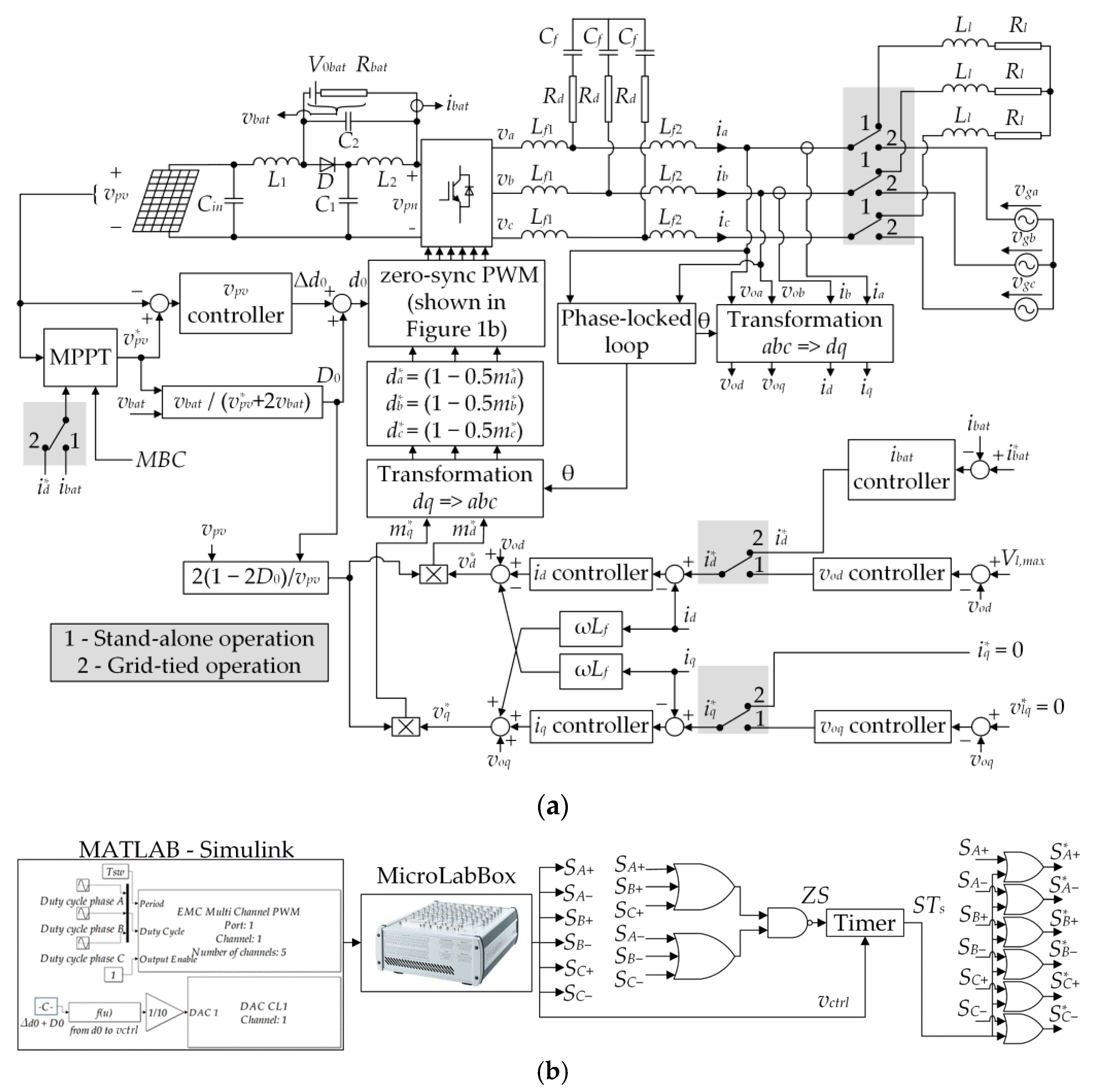
2. System Configuration

The considered PV system, including the corresponding control algorithm, is shown in Figure 1. The main components of the system are the PV source with the corresponding terminal capacitor Cin, the qZSI with the batteries added in parallel with the lower-voltage capacitor C2, and the three-phase output LCL filter, composed of inductors Lf1 and Lf2, capacitors Cf, and damping resistors Rd.
The control system of the qZSI is implemented in the d–q synchronous reference frame, with the inverter output voltages defined as follows [22]:
v o d = v d i d R f L f d i d d t + ω L f i q v o q = v q i q R f L f d i q d t ω L f i d
where vod, voq represent the d and q axis components of the inverter output voltage, respectively; vd, vq represent the d and q axis components of the inverter bridge output voltage, respectively; id, iq represent the d and q axis components of the inverter output current, respectively; ω is the angular frequency.
A properly selected bandwidth of the inverter output current controller ensures fairly accurate approximation of the LCL filter with the L filter [23], i.e., Lf = Lf1 + Lf2, Rf = Rf1 + Rf2, where Rf1 and Rf2 represent the corresponding parasitic resistances.

2.1. Grid-Tied Operation

During the grid-tied operation, the synchronous reference frame phase-locked loop (PLL) ensures the synchronization of the inverter output voltage with the grid voltage by maintaining vod = Vg,max and voq = 0, where Vg,max is the amplitude of the grid phase voltage. Note also that, during the grid-tied operation, the system angular frequency is equal to the grid angular frequency, where the angle θ required for the coordinate transformations is obtained as an integral of the angular frequency. The implementation of the PLL ensures the grid active (pgrid) and reactive power (qgrid) to be defined as follows [22]:
p g r i d = 3 2 i d V g , m a x q g r i d = 3 2 i q V g , m a x
During the grid-tied operation, the active power injected to the grid is defined by id, whereas the reactive power is defined by iq. The reference d-axis current (i*d) is obtained as the output of the battery current controller, whereas the reference q-axis current (i*q) is set to zero.

2.2. Stand-Alone Operation

During the stand-alone operation, two controllers are introduced to control voltages vod and voq. The reference of the d-axis voltage controller (v*od) is set equal to the amplitude of the phase load voltage (Vl,max). On the other hand, the reference q-axis voltage (v*oq) is set to zero in order to ensure the load active (pload) and reactive power (qload) to be defined as follows [22]:
p l o a d = 3 2 i d V l , m a x q l o a d = 3 2 i q V l , m a x
Note that, during the stand-alone operation, the angular frequency obtained by the phase-locked loop amounts to ω = 2πfl, where fl is the desired fundamental frequency of the load voltage/current (in this study, 50 Hz).

2.3. Maximum Power Point Tracking of the Photovoltaic Source

The I–V characteristics of the PV source are not linear and the electric power generated by the PV source varies with the irradiance and the temperature of the PV panels. However, there is an operating point where the PV source generates maximum power. Therefore, the MPPT algorithm is utilized to ensure the MPP operation of the PV source for different values of the solar irradiance and the PV panel temperature. In the considered system shown in Figure 1a, the proposed P&O MPPT algorithm tracks the MPP with the corresponding tracking period by varying the PV source voltage (vpv). The main advantage of this algorithm is that it does not require the measurement of the PV source current, which allows elimination of the corresponding sensor. During the grid-tied operation, the MPPT algorithm detects the MPP based on vpv and the reference d-axis grid current, whereas during the stand-alone operation it detects the MPP based on vpv and the battery current (ibat). Note that during the stand-alone operation, the battery current is not controlled, so in the case of the fully charged batteries, further charging has to be prevented. For that purpose, the maximum battery charge signal (MBC in Figure 1a) is implemented in the control algorithm. The detailed analysis of the proposed MPPT algorithm is given in Section 4.
In this study, the sinusoidal pulse-width modulation (PWM) with injected third harmonic and dead time is implemented [24]. The ST states are injected by means of the zero-sync PWM, proposed and detailed in [24], whose logic diagram is shown in Figure 1b. This method ensures wider range of the duty cycle and lower qZSI losses in comparison to the conventional ST states injection method without dead time.

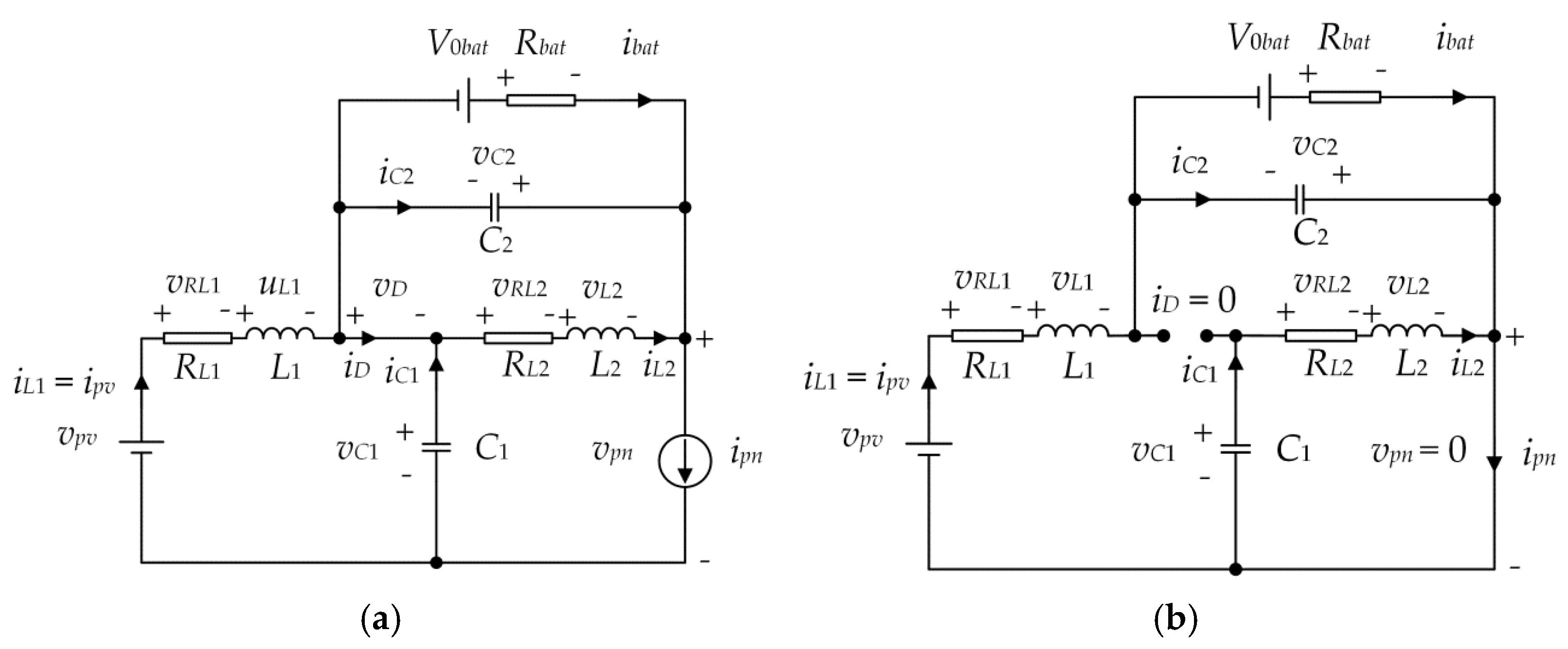
3. Small-Signal Model of the System

The small-signal model of the considered system is obtained by considering the equivalent circuits of the qZSI in the non-ST state and ST state, which are shown in Figure 2a,b, respectively. RL1 and RL2 represent the parasitic resistances of the impedance network inductors. Note that the influence of the terminal capacitor Cin is neglected, which implies that the PV source current (ipv) equals the qZSI inductor current (iL1). In this paper, a symmetrical impedance network is considered, i.e., L1 = L2 = L, C1 = C2 = C, RL1 = RL2 = RL. During the non-ST state, the impedance network is coupled to the load/grid, which allows the power flow from the PV source and the batteries to the load/grid. In this state, the diode D (Figure 1a) is forward biased, and the capacitors C1 and C2 are being charged, whereas the currents through L1 and L2 are decreasing. The dynamic state–space equations of the qZSI for the non-ST state, obtained based on Figure 2a, are given as follows:
F d x / d t = A n S T x + B n S T u
where
x = [ i L 1 i L 2 v C 1 i b a t ] T , u = [ v p v i p n V 0 b a t ] T ,
A n S T = [ R L 0 1 0 0 R L 0 R b a t 1 0 0 0 0 1 0 1 ] , B n S T = [ 1 0 0 0 0 1 0 1 0 0 1 0 ] , F = [ L 0 0 0 0 L 0 0 0 0 C 0 0 0 0 R b a t C ]
The state–space variables are the two inductor currents (iL1 and iL2), the voltage across C1 (vC1), and the battery current (ibat). The input variables of the model are the PV source voltage (vpv), the input current of the inverter bridge (ipn), and the battery open-circuit voltage (V0bat). Finally, the duty cycle (d0) is defined as T0/Tsw, where T0 and Tsw represent the ST state period and the switching period, respectively, whereas Rbat utilized in (4) represents the equivalent resistance of the batteries.
The ST state always occurs only during the zero-switching state, in which the impedance network is practically disconnected from the load/grid. During the ST state, the inverter bridge is short-circuited, which causes blocking of the diode D (Figure 1a), discharging of the capacitors C1 and C2, and an increase in iL1 and iL2. The utilization of the ST state ensures the boost of the PV source voltage. The dynamic state–space equations of the qZSI for the ST state are obtained, based on Figure 2b, as:
F d x / d t = A S T x + B S T u
where
A S T = [ R L 0 0 R b a t 0 R L 1 0 0 1 0 0 1 0 0 1 ] ,   B S T = [ 1 0 1 0 0 0 0 0 0 0 0 0 ] ,
The system average state–space equations are obtained by using state–space averaging, as follows:
F d x / d t = A x + B u
where
A = A S T d 0 + A n S T ( 1 d 0 ) = [ R L 0 d 0 1 d 0 R b a t 0 R L d 0 ( 1 d 0 ) R b a t 1 d 0 d 0 0 0 d 0 d 0 1 0 1 ]
B = B S T d 0 + B n S T ( 1 d 0 ) = [ 1 0 d 0 0 0 d 0 1 0 d 0 1 0 0 1 d 0 0 ]
The dynamic small-signal model of the considered system is obtained from the average state–space equations by utilizing the small-perturbation method and Laplace transformation. The I–V characteristic of the PV source may be described in the Laplace domain by utilizing the equivalent PV source resistance (Rfn), as follows [5,6]:
v ˜ p v ( s ) = R f n i ˜ L 1 ( s )
Finally, the average state–space equations in the Laplace domain, with the considered perturbation of the PV source voltage as per (7), are given as follows:
( R L + s L ) i ˜ L 1 ( s ) = ( D 0 1 ) v ˜ C 1 ( s ) R b a t D 0 i ˜ b a t ( s ) R f n i ˜ L 1 ( s ) + D 0 v ˜ 0 b a t + d ˜ 0 ( s ) V 11
( R L + s L ) i ˜ L 2 ( s ) = D 0 v ˜ C 1 ( s ) + ( 1 D 0 ) R b a t i ˜ b a t ( s ) + ( D 0 1 ) v ˜ 0 b a t + d ˜ 0 ( s ) V 11
C s v ˜ C 1 ( s ) = ( 1 D 0 ) i ˜ L 1 ( s ) D 0 i ˜ L 2 ( s ) + ( D 0 1 ) i ˜ p n ( s ) + d ˜ 0 ( s ) I 11
C s R b a t i ˜ b a t ( s ) = D 0 i ˜ L 1 ( s ) + ( D 0 1 ) i ˜ L 2 ( s ) i ˜ b a t ( s ) + ( 1 D 0 ) i ˜ p n ( s ) d ˜ 0 ( s ) I 11
In (7)–(11), capital letters represent the steady-state values of the considered variables, V11 = VC1IbatRbat + V0bat, I11 = Ibat − 2IL1 + Ipn, whereas “~” denotes the variables obtained as the Laplace transform of the corresponding perturbation (e.g., d ˜ 0 is equal to the Laplace transform of Δd0).
Equations (8)–(11) are used to obtain transfer functions which may be used for control system design. The first transfer function from the duty cycle to the PV source voltage is obtained from (8)–(11). However, the transfer functions from the duty cycle to the battery current and from the d-axis grid current to the battery current require one more equation. In the non-ST state, this equation is defined as:
i p n V p n = 3 2 v o d i d
where Vpn represents the peak value of the inverter bridge input voltage of the ideal qZSI.
In (12), the input power of the inverter bridge is assumed equal to the inverter output power expressed in the dq coordinate system, which implies neglecting of the inverter bridge losses and output LCL filter losses.
In the ST state, there is no exchange of energy between the ac and dc sides of the inverter bridge. Consequently, the average equation is obtained by multiplying the inverter input power during the non-ST state (left side of (12)) with the factor (1 − d0), as follows:
i p n V p n ( 1 d 0 ) = 3 2 v o d i d
In (13), vod may be obtained as a function of Vpn and the amplitude modulation index (ma), as follows:
v o d = V p n 2 m a
With respect to (14), (13) becomes:
i p n ( 1 d 0 ) = 3 4 m a i d
By utilizing the small-perturbation method and Laplace transformation, (15) becomes:
i ˜ p n ( s ) ( 1 D 0 ) d ˜ 0 ( s ) I p n = 3 4 m ˜ a ( s ) I d + 3 4 M a i ˜ d ( s )
where capital letters represent the steady-state values of the considered variables.
The transfer function from the d-axis grid current to the battery current is obtained based on (8)–(11) and (16). In the five considered equations, there are nine variables, so in order to obtain the desired transfer function, the perturbances of three variables should be set to zero. It is assumed that, during the perturbation of the d-axis grid current, the modulation index, the open-circuit voltage of the batteries, and the duty cycle remain constant. Finally, with m ˜ a ( s ) = 0 , v ˜ 0 b a t ( s ) = 0 , and d ˜ 0 ( s ) = 0 , the transfer function from the d-axis grid current to the battery current is given as follows:
G i ˜ d i ˜ b a t = 1 4 N 3 s 3 + N 2 s 2 + N 1 s + N 0 K 4 s 4 + K 3 s 3 + K 2 s 2 + K 1 s + K 0
where
N 0 = 3 M a R L + 3 D 0 M a R f n ,   N 1 = 3 M a L + 3 C M a R L 2 + 3 C M a R f n R L ,
N 2 = 6 C M a L R L + 3 C M a R f n L ,   N 3 = 3 C M a L 2 ,
K 0 = 2 D 0 2 R L + 4 D 0 2 R b a t + D 0 2 R f n 2 D 0 R L 4 D 0 R b a t + R L + R b a t
K 1 = L 2 D 0 L + 2 D 0 2 L + C R L 2 + 2 C R L R b a t + C R L R f n + C R b a t R f n + 4 C D 0 2 R L R b a t + 2 C D 0 2 R b a t R f n 4 C D 0 R L R b a t 2 C D 0 R b a t R f n
K 2 = 2 C L R L + 2 C L R b a t + C L R f n + C 2 R L 2 R b a t 4 C D 0 L R b a t + 4 C D 0 2 L R b a t + C 2 R L R b a t R f n
K 3 = C L 2 + 2 C 2 L R L R b a t + C 2 L R b a t R f n ,   K 4 = C 2 L 2 R b a t .
The transfer function obtained in (17) is required for the design of the battery current control loop utilized during the grid-tied operation. On the other hand, the transfer function from the duty cycle to the battery current was obtained from (8)–(11) and (16), by considering the assumptions v ˜ 0 b a t ( s ) = 0 , m ˜ a ( s ) = 0 , i ˜ d ( s ) = 0 , as follows:
G d ˜ 0 i ˜ b a t = 1 4 P 3 s 3 + P 2 s 2 + P 1 s + P 0 K 4 s 4 + K 3 s 3 + K 2 s 2 + K 1 s + K 0
where
P 0 = 4 V 11 + 8 D 0 V 11 4 I 11 R L + 4 I p n R L 4 D 0 I 11 R f n + 4 D 0 I p n R f n ,
P 1 = 4 I 11 L + 4 I p n L 4 C R L V 11 4 C R f n V 11 4 C I 11 R L 2 + 4 C I p n R L 2 + + 8 C D 0 R L V 11 + 4 C D 0 R f n V 11 4 C I 11 R L R f n + 4 C I p n R L R f n
P 2 = 4 C L V 11 + 8 C D 0 L V 11 8 C I 11 L R L 4 C I 11 L R f n + 8 C I p n L R L + 4 C I p n L R f n ,
P 3 = 4 C I 11 L 2 + 4 C I p n L 2
The transfer function given in (18) was utilized only for the selection of the MPPT algorithm tracking period (Tmppt) because the longest settling time of the battery current response is noted for step changes in the duty cycle. Note that the transfer function from the duty cycle to the battery current has been already derived in [13,14,15], but errors have been detected in the corresponding small-signal model. First, in the system of Equation (5) in [14], (1–d0)V0bat in the second equation should be replaced by (d0−1)V0bat. The second detected error is the utilization of an equation that defines the steady-state battery current for the determination of the dynamic model of the system.
The transfer function from d0 to vpv is obtained from (8)–(11), by considering the assumptions i ˜ b a t ( s ) = 0 and v ˜ 0 b a t ( s ) = 0 . This transfer function is required for the design of the PV source voltage control loop for both the grid-tide and stand-alone operation, and it is expressed as follows:
G d ˜ 0 v ˜ p v = R f n G d ˜ 0 i ˜ L 1 = R f n C L V 11 s 2 + C R L V 11 s + V 11 C L 2 s 3 + ( 2 C L R L + C R f n L ) s 2 + ( L + C R L 2 + C R f n R L ) s + R L + D 0 R f n
The steady-state values of the state–space variables are obtained from (6), by setting the right side equal to zero, as follows:
I L 1 = d 0 I b a t ( d 0 1 ) I p n 1 2 d 0 I L 2 = ( d 0 1 ) I b a t ( d 0 1 ) I p n 1 2 d 0 I L 1 I L 2 = I b a t V C 1 = 1 d 0 1 2 d 0 V p n + 2 d 0 ( 1 d 0 ) R L I b a t ( 1 d 0 ) R L I p n ( 1 2 d 0 ) 2 V C 2 = d 0 1 2 d 0 V p n + ( 2 d 0 2 2 d 0 + 1 ) R L I b a t + ( d 0 1 ) R L I p n ( 1 2 d 0 ) 2
In the case RL = 0, the expressions for the voltages VC1 and VC2 obtained from (20) are equal to the expressions well-known from the literature [4]. The steady-state values obtained in (20) differ from those obtained in [13,14,15] due to the above-described errors in the corresponding small-signal model.

4. Control Schemes for the Grid-Tied Operation and Stand-Alone Operation

The control algorithm of the considered PV system deals with multiple tasks. During the grid-tied operation, the battery current is controlled through the adjustment of the reference d-axis grid current. On the other hand, during the stand-alone operation, the d and q axis components of the load voltage are controlled through the adjustment of the corresponding reference d and q axis currents, respectively. In both the considered cases, the PV source power is controlled through the adjustment of the PV source voltage. The detailed analysis of the respective control loops is given below.

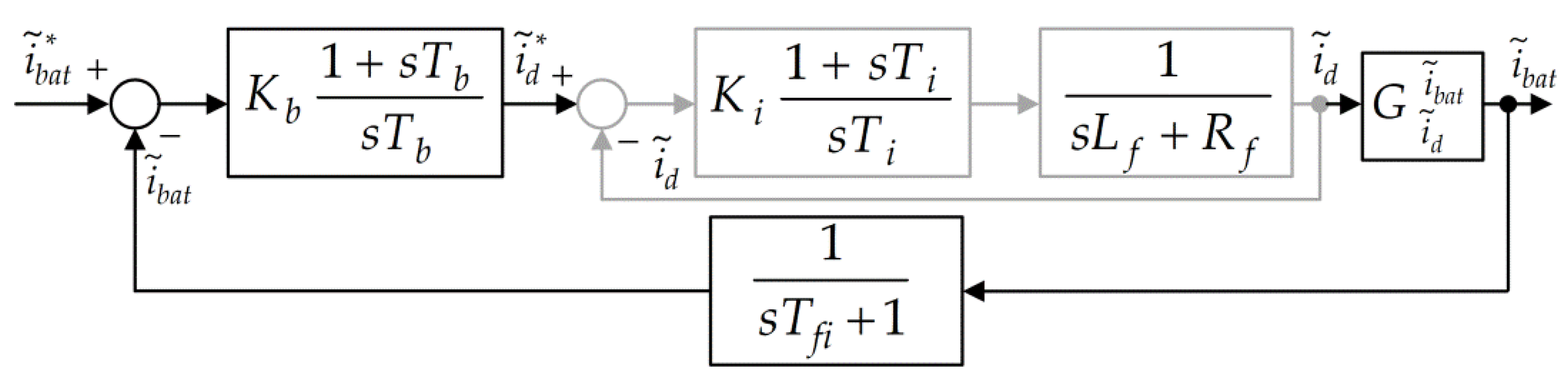
4.1. Control of the Battery Current for the Grid-Tied Operation

The battery current control loop is shown in Figure 3. The output value of the battery current controller is the reference d-axis grid current (i*d), which practically means that the battery controller controls the active power injected to the grid. The inner control loop—highlighted in grey in Figure 3—contains the d-axis current controller and the transfer function of the output filter, with neglected dynamics of the inverter bridge. Note that the output filter was modeled as an L filter (Lf = Lf1 + Lf2, Rf = Rf1 + Rf2) since the properly selected bandwidth of the d-axis current controller ensures fairly accurate approximation of the LCL filter with the L filter [23]. The transfer function from the d-axis grid current to the battery current given in (17) was utilized to obtain the battery current, which is then filtered by the first order filter in the feedback loop.
The q-axis grid current control loop is identical to the inner control loop shown in Figure 3, including the values of the controller parameters, with the corresponding reference value (i*q) set to zero to ensure zero reactive power.

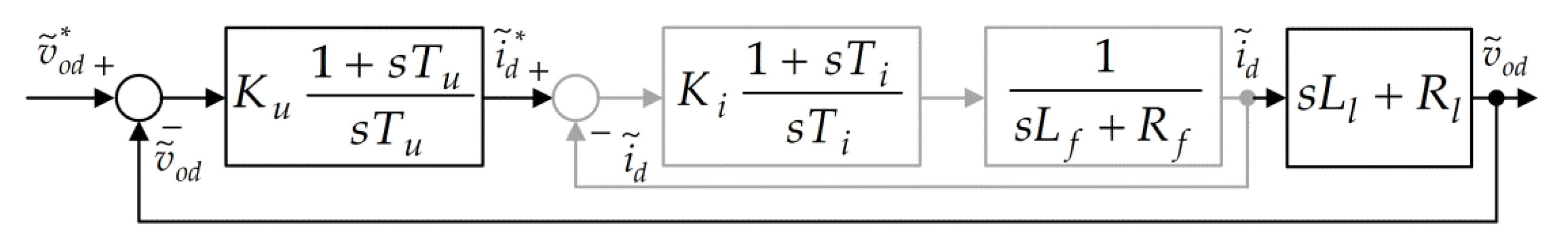
4.2. Control of the Inverter Output Voltage for the Stand-Alone Operation

Figure 4 shows the control loop of the d-axis load voltage (vod) during the stand-alone operation. The reference d-axis voltage (v*od) defines the amplitude of the phase load voltage since the reference q-axis voltage (v*oq) is set to zero, as shown in Figure 1a. The output value of the voltage controller in Figure 4 is the reference d-axis load current. The corresponding inner loop in Figure 4 is the same as that for the grid-tied operation (Figure 3), including the values of the current controller parameters. The transfer function of the load is utilized to obtain vod from id. The load is modeled as a resistive–inductive load with the corresponding inductance Ll and the resistance Rl.
The same control loop as in Figure 4 is utilized for the load q-axis voltage during the stand-alone operation, including the values of the controllers’ parameters. Due to the fact that v*oq equals zero, the reference q-axis current (i*q) defines the reactive power required by the load. This means that, in the case of the resistive load, the q-axis current will be equal to zero, whereas in the case of the resistive–inductive load, this current will be negative.

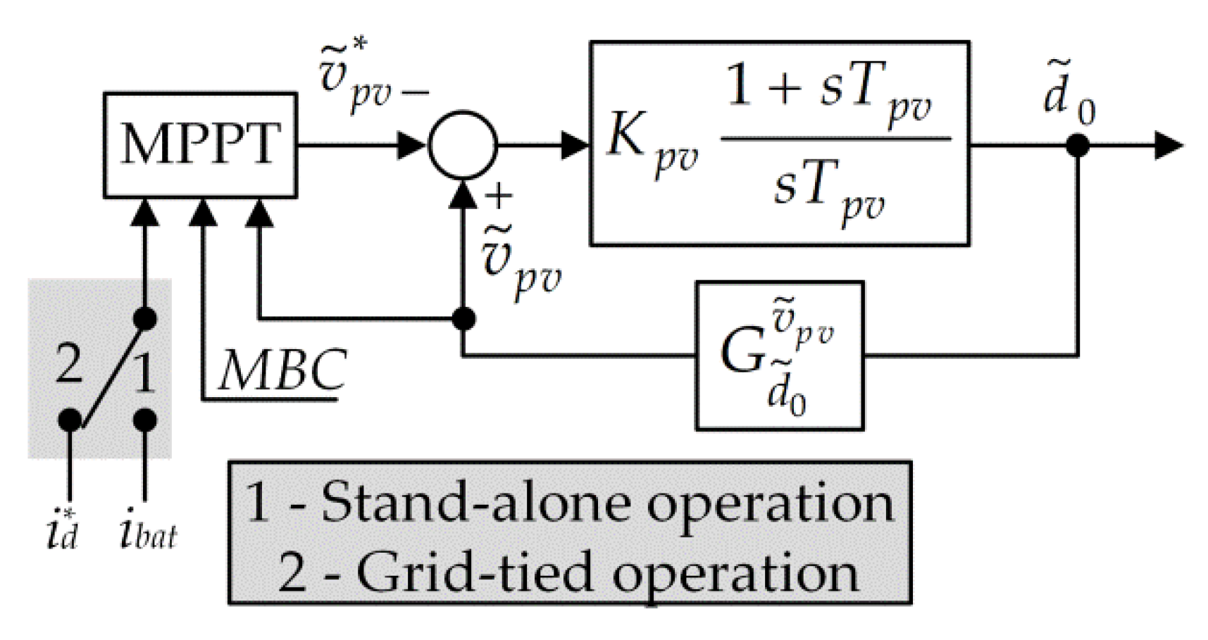
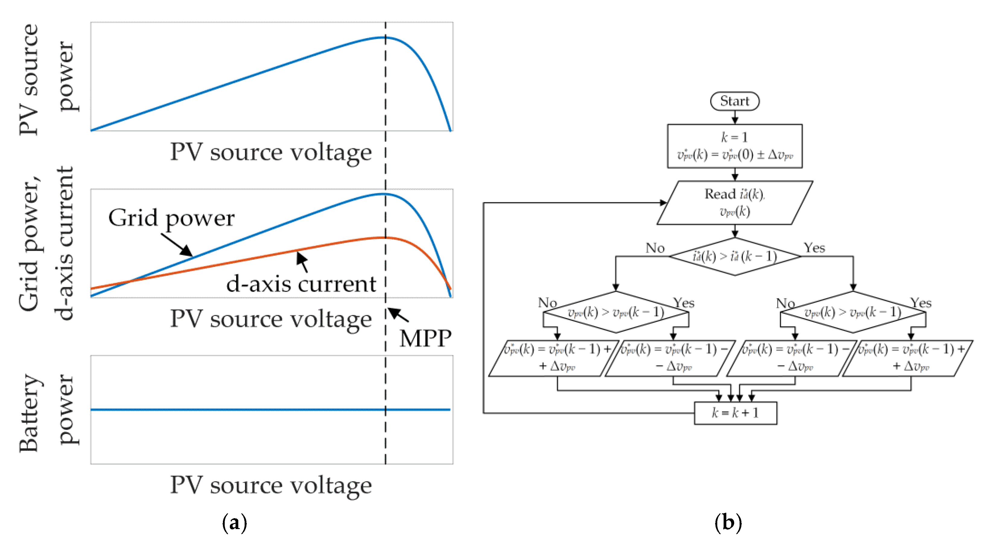
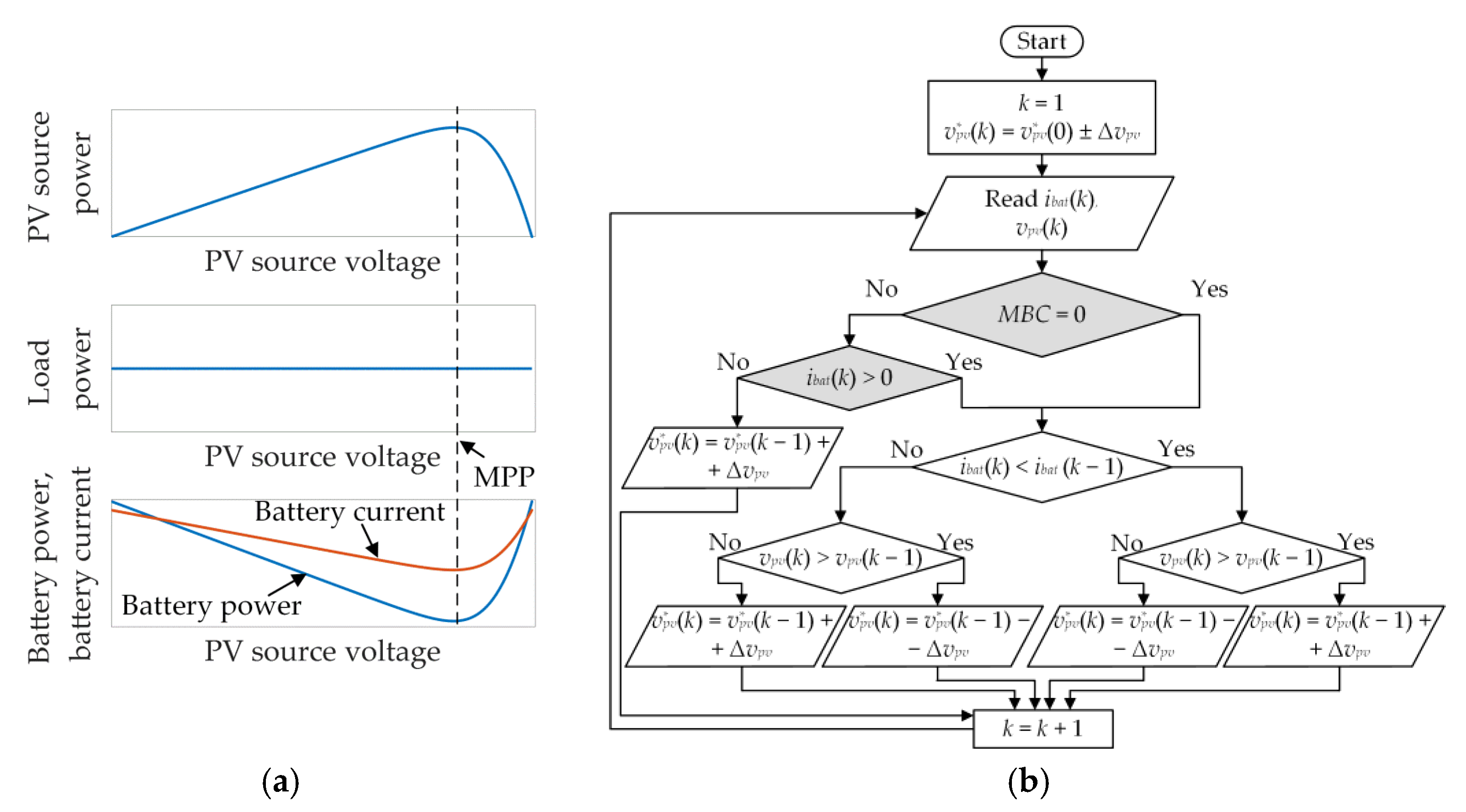
4.3. Control of the Photovoltaic Source Voltage and Maximum Power Point Tracking

The control loop of the PV source voltage is shown in Figure 5. The reference PV source voltage (v*pv) is provided by the MPPT algorithm, whereas the output signal of the respective voltage controller is the duty cycle. The transfer function from the duty cycle to the PV source voltage, given in (19), is utilized to obtain the PV source voltage based on the duty cycle. The control scheme shown in Figure 5 is utilized for the tuning of the PV source voltage controller.
As shown in Figure 5, the PV source voltage is controlled by varying the duty cycle, which is enabled by connecting the batteries in parallel with C2, yielding [4]:
V b a t = V C 2 = d 0 1 2 d 0 V p v
where the mean values of the considered variables are denoted by capital letters.
The battery voltage (Vbat) is approximately constant, so the variation of the duty cycle (d0) results in the variation of Vpv. The equivalent duty cycle is obtained as the sum of the duty cycle obtained by the controller and the corresponding feed-forward signal (D0) obtained according to (21) as Vbat/(V*pv + 2Vbat).
In the conventional P&O MPPT algorithm, the MPP is achieved by considering the PV source voltage and power, which requires the measurement of the PV source voltage and current. The P&O MPPT algorithm proposed in this study requires the PV source voltage and the reference d-axis grid current during the grid-tied operation, whereas it requires the PV source voltage and the battery current during the stand-alone operation. In this way, the PV source current sensor is omitted. In addition, the currents i*d and ibat are required by the control algorithm, regardless of the MPPT algorithm. This means that the number of required sensors in the system is reduced by one. Note also that the MBC signal is implemented in the control algorithm in order to disable charging of the already fully charged batteries during the stand-alone mode. In the case of MBC = 0, battery charging is enabled and the system operates in the MPP, whereas in the case of MBC = 1, the battery current is limited to values higher than or equal to zero to prevent further charging. Therefore, the system operating point may depart from the MPP in the case of MBC = 1.
Figure 6a shows the PV source power (ppv), the grid power (pgrid), the d-axis grid current, and the battery power (pbat) during the grid-tied operation. In this case, the battery current is considered constant since the battery current reference is set to a constant value. The power relation during the grid-tied operation with omitted power losses is defined as follows:
p p v + p b a t = p g r i d v p v i p v + i b a t v b a t = 3 2 V g , m a x i d
The constant battery power means that the variation of the grid injected power follows the variation of the PV source power (the power losses may also be assumed to change proportionally to the PV source power). Hence, the variation of pgrid with vpv is the same as the variation of ppv with vpv, as shown in Figure 6a. The MPP of the PV source power corresponds to the MPP of the grid injected power, so ppv may be replaced by pgrid in the MPPT algorithm. Finally, pgrid may be replaced by the reference d-axis grid current since the grid voltage is considered constant (Vg.max = const.). Note that the system is robust to a grid voltage sag, since Tmppt amounts to a few hundred ms. Figure 6b shows the flow chart of the MPPT algorithm during the grid-tied operation. As compared to the conventional P&O algorithm, the PV source power is here replaced by the reference d-axis grid current.
Figure 7a shows the PV source power (ppv), the load power (pload), the battery power (pbat), and the battery current during the stand-alone operation. In this case, the load power is considered to be slowly varying in comparison with the PV source dynamics, so it may be regarded as constant during the PV source power variation. The power balance equation for the stand-alone operation with omitted power losses is defined as follows:
p p v = p l o a d p b a t v p v i p v = 3 2 V l , m a x i d i b a t v b a t
The constant load power means that the variation of the battery power follows the variation of the PV source power. During battery discharge, the battery power decreases with the increase in the PV source power, whereas during charging, although its absolute value increases with the increase in the PV source power, the battery power changes sign and actually continues to decrease in value. Therefore, in both considered battery modes, the maximum PV source power corresponds to the minimum battery current, as shown in Figure 7a. Consequently, during the stand-alone operation, the PV source power may be replaced by the battery power in the MPPT algorithm. Finally, the battery power may be replaced by the battery current provided that the battery voltage is considered as approximately constant.
Figure 7b shows the flow chart utilized for the determination of the PV source reference voltage (v*pv) during the stand-alone operation, which consists of two parts. The first part is the proposed P&O algorithm, where the PV source power is replaced with the battery current. The second part encompasses conditions added to prevent overcharge of the batteries, which are grey colored in Figure 7b. In the case when the battery charging is allowed, the MBC value equals 0 and v*pv is set to achieve the MPP. However, in the case when the batteries are fully charged, the MBC value equals 1 and v*pv is set to ensure that the battery current does not drop below zero, thus preventing further charging. In the case when MBC = 1 and the battery current is negative, the reference PV source voltage is increased, which, in turn, causes the decrease in the PV source power (i.e., the new PV source operating point is placed right of the MPP on the I–V (or P–V) characteristics of the PV source). The battery current eventually oscillates at around zero. The corresponding mean value may slightly differ from zero, but this error is practically negligible and it may be further reduced by decreasing the variation step of v*pvvpv). Note that the PV source power could be alternatively decreased by decreasing the reference voltage (i.e., by placing the operating point left of the MPP). However, the first-mentioned approach results in lower current ripple and power losses and was, hence, utilized in this study.

5. Experimental Implementation of the System

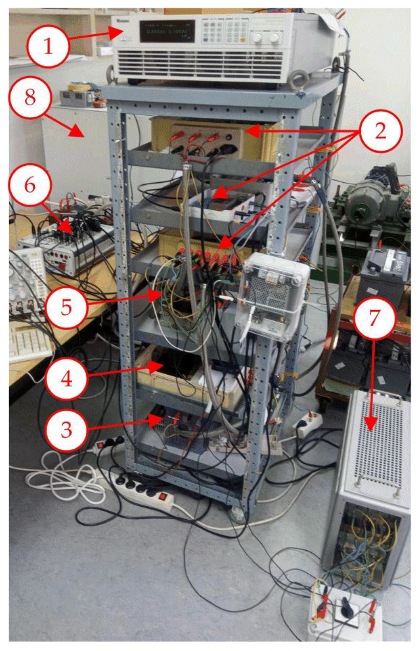
5.1. Laboratory Setup

Figure 8 shows the laboratory setup of the considered PV system. The main components are denoted as follows:
  • DC power supply Chroma 62050H 600S, programmed to emulate 16 series-connected PV panels KC200GT (Kyocera).
  • Hall-effect transducers LA 55-P/SP52 [25] (for the battery current and the grid/load phase currents), DVL 500 [26] (for the PV source voltage), CV 3–500 [27] (for the grid voltages), and LV 25-P (for the load voltages) (LEM).
  • qZSI impedance network with L1 = L2 = 20.2 mH (unsaturated), RL = 0.5 Ω (at 25 °C)), and C1 = C2 = 50 μF (ESR = 7.8 mΩ).
  • qZSI three-phase inverter bridge (IXBX75N170 IGBTs (IXYS) and SKHI 22B(R) drivers (Semikron)).
  • LCL filter at the qZSI output stage (Lf1 = 8.64 mH, Lf2 = 4.32 mH, Rf1 = 0.1036 Ω, Rf2 = 0.0518 Ω, Cf = 4 μF, Rd = 10 Ω), with the design details given in Appendix A.
  • MicroLabBox controller board (dSpace) for the qZSI control.
  • A symmetric three-phase resistive load.
  • The battery system composed of 22 lead-acid batteries connected in series with a total open-circuit voltage amounting to about 270 V.
The major part of the control algorithm was executed with the sampling frequency of 10 kHz. Exceptions are the MPPT algorithm—executed with 5 Hz—and the battery current sampling and filtering—executed with 20 kHz—with the time constant of the corresponding first-order filter (Tfi) set to 5 ms. In this way, the steady-state error of the measured battery current—that otherwise exists when the battery current waveform is sampled with lower frequencies—is eliminated. The sampling frequency of the MPPT algorithm (fmppt = 1/Tmppt) was chosen so as to ensure that all the corresponding transients disappear within a single sampling interval. Note that fmppt has to be a multiple of the sampling frequencies of 10 kHz and 20 kHz due to the multitask operation of MicroLabBox.
The synchronous reference frame PLL with the moving average filter (MAF) [28] was utilized in this study during the grid-tied operation. The corresponding controller parameters have been set to Kpll = 0.0464 rad/Vs and Tpll = 0.02 s, whereas the MAF widow was set to 0.01 s in order to completely remove the 100 Hz harmonics and all its multiples from the filtered voq [29].
The duty cycle (d0) is converted into the control voltage (vctrl) of the LM555CN timer, which results in the desired T0 (Figure 1b). The equation that defines vctrl according to d0 is given as follows [24]:
v c t r l = V c c ( 1 e d 0 T s w / 2 T t ) = V c c ( 1 e T 0 / 2 T t )
where Vcc represents the supply voltage of the timer (5 V in this study), Tt represents the corresponding time constant (20.8 μs in this study), and Tsw is set to 0.2 ms in this study.

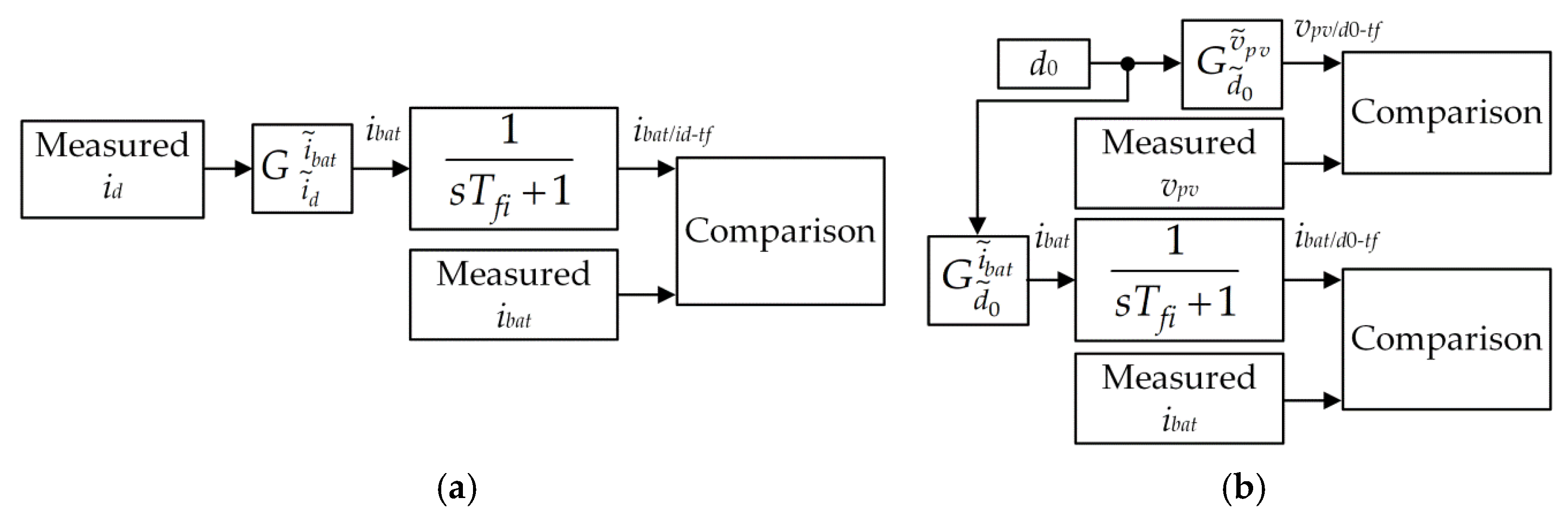
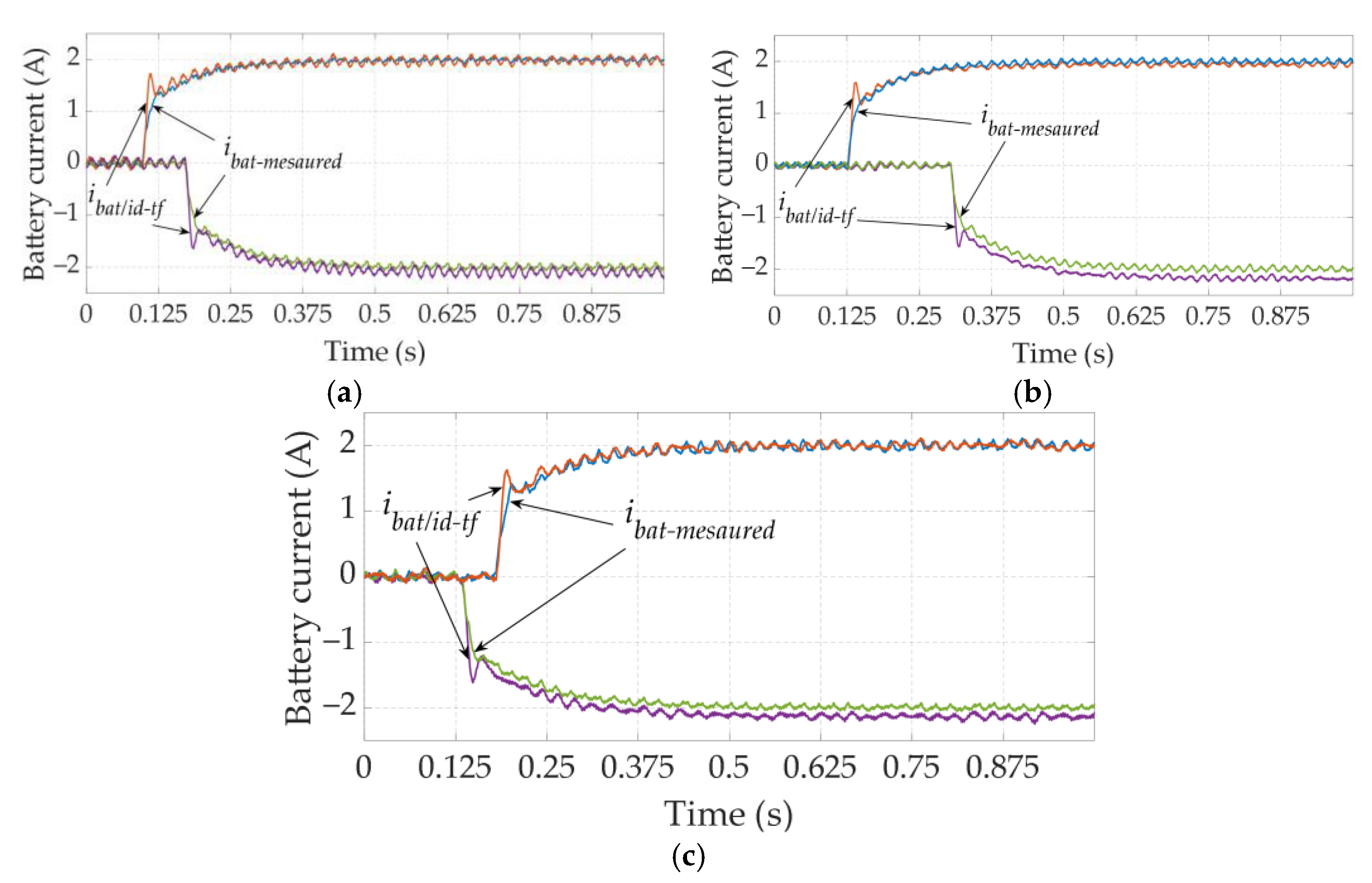
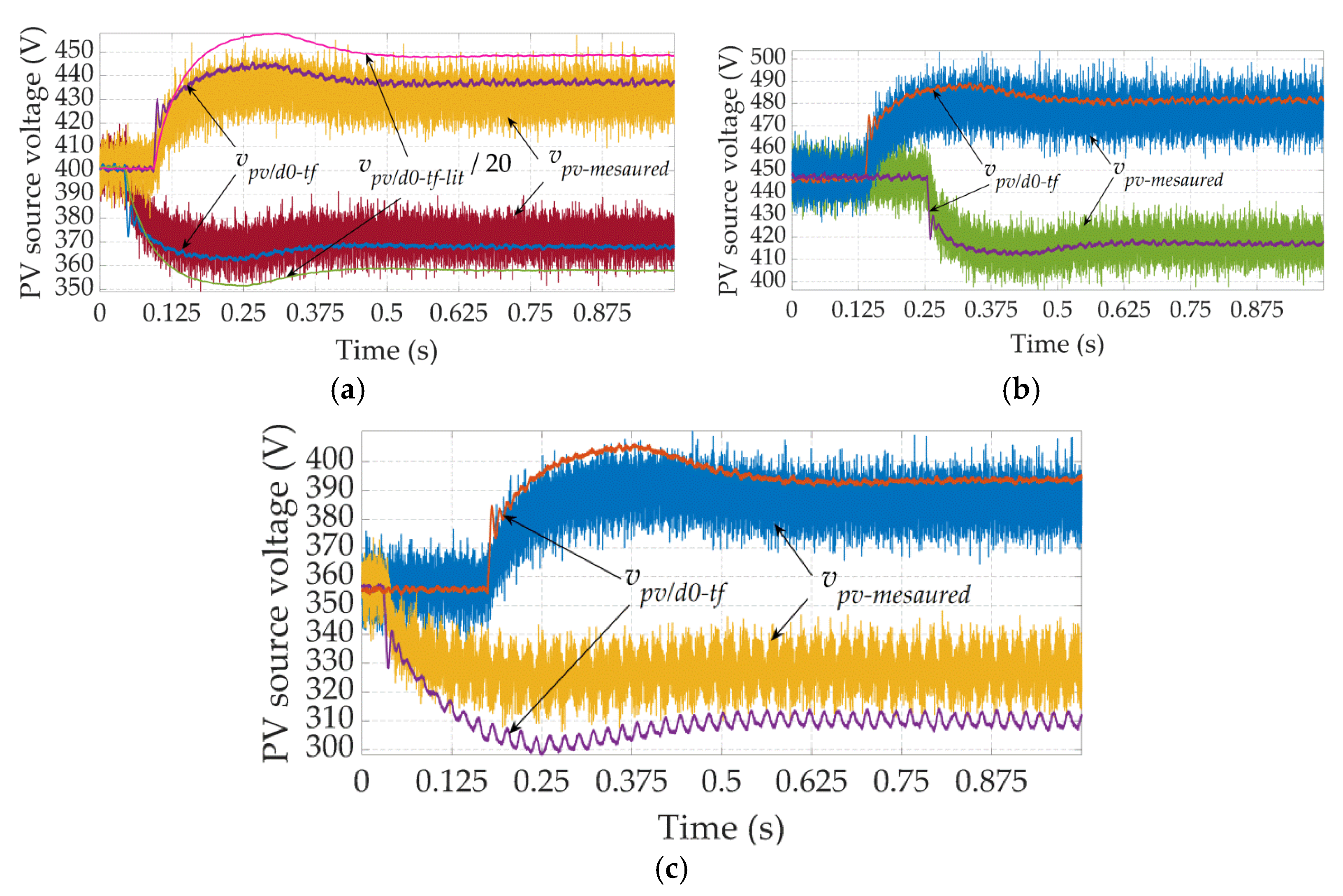
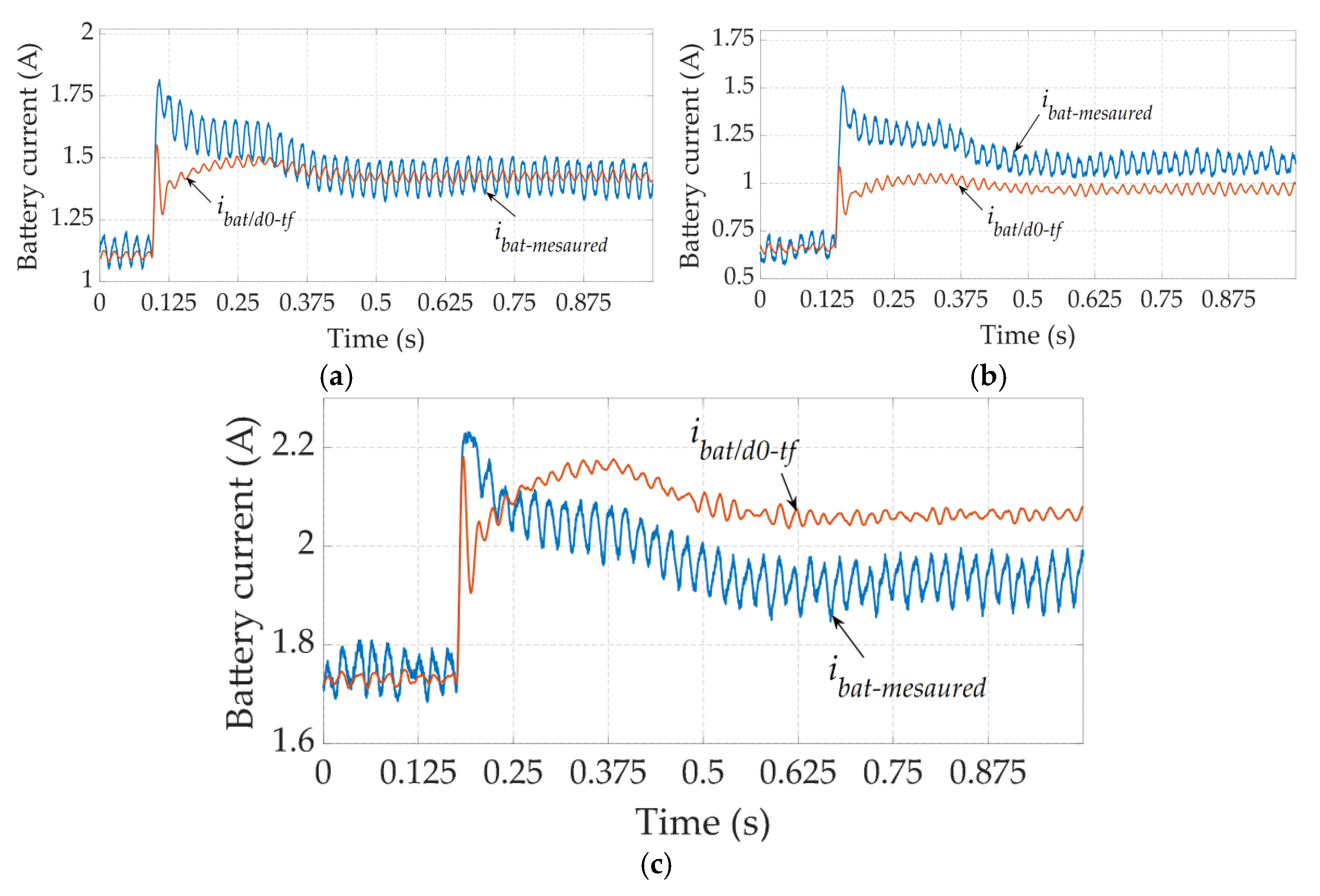
5.2. Accuracy Verification of the Proposed Transfer Functions

The accuracy verification of the proposed transfer functions was carried out by comparison of the waveforms calculated by means of the transfer function with those obtained by measurement. Figure 9a shows the setup utilized for the verification of the transfer function from id to ibat. The input signal of the transfer function is the measured waveform of id, whereas the output signal denoted as ibat is the calculated battery current, which is then filtered with the same first-order filter as the measured battery current (ibat-measured). Finally, the filtered calculated battery current denoted as ibat/id-tf is compared with the filtered measured battery current. Note that all the measurements for the verification of the transfer function from id to ibat were carried out during the grid-tied operation for the constant PV source power.
Figure 9b shows the setup utilized for the verification of the transfer functions from d0 to ibat and from d0 to vpv. The input signal for both the considered transfer functions—the duty cycle (d0)—is determined by the control algorithm. The output signal of the transfer function from d0 to vpv (vpv/d0-tf) is compared with the measured vpv (vpv-measured), whereas the filtered output signal of the transfer function from d0 to ibat (ibat/d0-tf) is compared with the filtered measured battery current ibat-measured. These two transfer functions were tested during the stand-alone operation for the constant load power.
The accuracy verification of the transfer function from id to ibat was carried out for three different combinations of the irradiance value (Z) and the PV panels’ temperature (Tpv). The linearization of the considered transfer function was carried out for Z = 600 W/m2 and Tpv = 30 °C. These values represent the approximate average values of Z and Tpv encompassed in the measurements in this study (i.e., Z is varied from 300 W/m2 to 1000 W/m2, whereas Tpv is varied from 10 °C to 50 °C). The linearization was carried out in the MPP, where the input parameters of the transfer function from id to ibat, defined in (17), are given in Table 1.
The value of Rfn is obtained for the considered operating point based on the corresponding I–V characteristic of the PV source, whereas the Rbat value corresponds to the internal resistance of 22 lead-acid batteries connected in series.
Figure 10 shows the comparison of ibat-measured and ibat/id-tf for the step variations of i*d of ±2 A in three different operating points. First, the id value was varied in the linearization point (Z = 600 W/m2, Tpv = 30 °C) and the corresponding waveforms are shown in Figure 10a. The maximum steady-state error in this case amounts to 4%. The transfer function accuracy was also tested for two operating points different than the linearization point. The waveforms shown in Figure 10b were recorded for Z = 1000 W/m2 and Tpv = 10 °C, and the waveforms shown in Figure 10c were recorded for Z = 500 W/m2 and Tpv = 50 °C. The maximum steady-state error in Figure 10b,c amounts to 10.5% and 8%, respectively.
The accuracy verification of the transfer functions from d0 to ibat and from d0 to vpv— (18) and (19), respectively—was carried out for three values of Tpv and with Z set to 600 W/m2. The linearization of these two transfer functions was carried out in the MPP, with the input parameters given in Table 2.
Figure 11 shows the comparison of vpv-measured and vpv/d0-tf for the step variations of d0 of ±0.011, for three different operation points. First, the variation of d0 was carried out in the linearization point (Z = 600 W/m2, Tpv = 30 °C) and the corresponding waveforms are shown in Figure 11a. The maximum steady-state error in this case amounts to 1.6%. In the case of Tpv = 10 °C and Tpv = 50 °C, waveforms shown in Figure 11b,c, respectively, the maximum steady state error amounts to 2.5% and 4.3%, respectively.
In Figure 11a, waveforms denoted as vpv/d0-tf-lit were obtained by the utilizing the transfer function taken from the literature [11], with the input parameters taken from Table 2. Note that vpv/d0-tf-lit had to be reduced 20 times in order to fall within the range in Figure 11a. This huge error in the obtained result suggests that the transfer function reported in [11] probably contains one or more overlooked errors.
Figure 12 shows the comparison of ibat-measured and ibat/d0-tf for the step variation of d0 of −0.011, for three different operation points. The lowest maximum steady-state error of approximately 4% is noted for the linearization point shown in Figure 12a (Z = 600 W/m2, Tpv = 30 °C). In the case of Tpv = 10 °C and Tpv = 50 °C with Z = 600 W/m2—waveforms shown in Figure 12b,c, respectively—this error amounts to approximately 12%. It is assumed this error is a consequence of the variation of ma and ipn with the duty cycle, whereas the transfer function defined in (18) is derived with both ma and ipn considered as constant. However, the transfer function from d0 to ibat is only utilized for the determination of the MPPT algorithm tracking period (Tmppt). Therefore, the estimation of the steady-state value by the considered transfer function is not as important as the estimation of the settling time. Figure 12 shows that the settling time of ibat/d0-tf is approximately the same as the settling time of ibat-measured for all the considered operation points. This approves the utilization of the transfer function from d0 to ibat for the determination of Tmppt, since the longest settling time of the battery current response is noted for step changes in the duty cycle.

5.3. Tuning of the PI Controllers

The high noted accuracy of the transfer functions from id to ibat and from d0 to vpv allows the control loops shown in Section 4 to be utilized for the tuning of the system controllers. The d- and q-axis current controllers in the inner loops in Figure 3 and Figure 4, respectively, were tuned according to the recommendation in [22]. However, it was important to ensure the bandwidth of these current loops to be lower than the resonant frequency of the LCL filter, which is defined as follows [23]:
f r e s = 1 2 π L f 1 + L f 2 C f L f 1 L f 2 = 1200   Hz
The parameters of id and iq PI controllers are calculated as follows:
K i = L f 1 + L f 2 τ i = 0.01296 0.0005 = 25.92   V / A T i = L f 1 + L f 2 R f 1 + R f 2 = 0.01296 0.1545 = 0.084   s
The parameter τi in (26) was set to 0.5 ms in order to ensure the fast response of id and iq without the overshoot. The bandwidth of the current control loops with the utilized controller parameters from (26) amounts to 337 Hz, which is significantly lower than fres = 1200 Hz. In this way, the approximation of the LCL filter with the L filter is justified.
The parameters of the battery current controller were determined based on the battery current control loop shown in Figure 3, by considering the corresponding Bode plot shown in Figure 13. The gain of the battery current open loop (Go-ibat) was compensated by the corresponding PI controller (GPI-ibat) in order to achieve the fast response of the battery current and stable operation of the system. The controller parameters of Kb = 0.446, Tb = 0.04 s were selected to ensure the amplitude margin (AM) of the open-loop characteristic (Go-ibat-PI) not lower than 10 dB. This resulted in the high phase margin (PM) of 132°.
Figure 14 shows the Bode plot of the d-axis voltage control loop shown in Figure 4. The gain of the open loop without implemented PI controller (Go-vod) was compensated by the PI controller gain (GPI-vod) in order to ensure high crossover frequency and satisfactory phase margin of the resulting open-loop characteristic (Go-vod-PI). The phase margin of 69° at the crossover frequency of 1000 rad/s was achieved by utilizing the controller parameters Ku = 0.00186 A/V, Tu = 9.99∙10−5 s. This analysis was carried out with the pure resistive, star-connected load of Rt = 53 Ω, resulting in approximately the nominal output power of 3 kW. Note that for the resistive–inductive load, the phase margin becomes even higher, whereas for higher Rt values (i.e., for power lower than nominal), the phase margin slightly decreases.
Figure 15 shows the Bode plot of the PV source voltage control loop shown in Figure 5. The corresponding PI controller (GPI-vpv) was utilized to compensate the gain of the PV source voltage open loop (Go-vpv) and to ensure fast response, with overshoots not higher than 10% in order to maintain stable operation of the system. The controller parameters Kpv = 1.88∙10−4 V−1 and Tpv = 0.0166 s ensure the phase margin of 52° of the compensated open-loop characteristics (Go-vpv-PI), which is considered satisfactory.
As for the MPPT algorithm, the corresponding fixed variation step of v*pvvpv) was set to 5 V. For this value of Δvpv, the longest transient, of approximately 0.15 s, is noted for the transfer function from d0 to ibat. Finally, Tmppt is set to 0.2 s in order to ensure the proper multitask operation of MicroLabBox, as explained above.
The parameters given above were implemented into the system, which was tested both during the grid-tied operation and the stand-alone operation. The results are presented in the next section.

6. Experimental Results

The experimental testing of the considered system was carried out for different operation conditions. During the experimental testing, the irradiance value was varied from 300 W/m2 to 1000 W/m2, whereas the PV source temperature was varied from 10 °C to 50 °C. First, the steady-state analysis was carried out to determine the basic features of the considered system, including the accuracy of the proposed MPPT algorithm, the system power distribution, and the efficiency, as well as to gain a more complete insight into the operation of the system. The dynamic analysis of the system, on the other hand, is crucial for the validation of the proposed concept, so it was carried out in a more meticulous way in order to determine the system response with respect to the variation of different system variables, such as the irradiance or the load-resistance value. Note that the value of the PV source power is not required by the proposed control algorithm. Therefore, the PV source power calculation is enabled only in order to determine the static tracking efficiency of the proposed MPPT algorithm. The PV source current has been measured for this purpose by means of the Hall-effect transducers LA 55-P/SP52 (LEM).

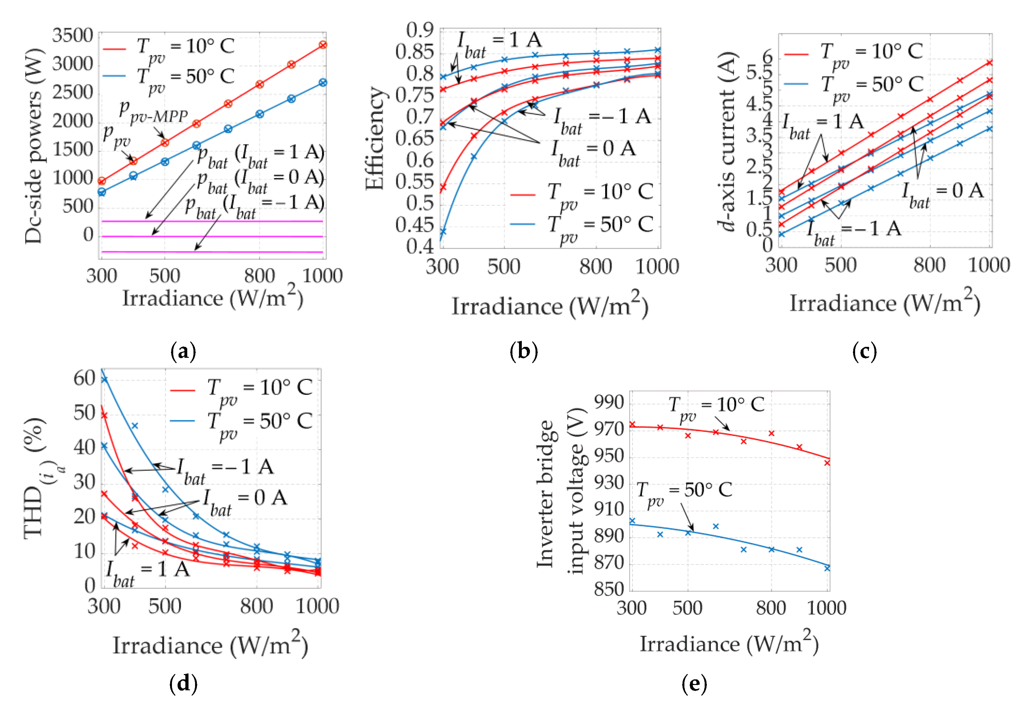
6.1. Steady-State Analysis

The steady-state results are shown in Figure 16. The measurements were carried out during the grid-tied operation for the temperatures Tpv = 10 °C and Tpv = 50 °C, and for all the considered irradiances. The reference battery current was varied in order to achieve different battery power values and, hence, different values of the grid power and current. The increase in the positive (discharging) battery power (pbat) results in an increase in the d-axis current injected to the grid (id) for approximately the value of Δpbat/(1.5Vg,max), whereas the increase in the negative (charging) battery power results in the decrease in id for approximately the value of Δpbat/(1.5Vg,max). Note that the inverter losses remain practically constant during the variation of pbat. As expected, the achieved PV source power (ppv), denoted “x” in Figure 16a, is higher for Tpv = 10 °C than for Tpv = 50 °C. This power is practically equal to the maximum available PV power (ppv-MPP), denoted “o” in Figure 16a, for all the considered operating points. The static tracking efficiency (STE) of the proposed P&O algorithm calculated as Ppv/Ppv-MPP for all the considered measurement points is shown in Table 3. The considered efficiency ranges from 96.9% to 100%, which corresponds to the values given in [30,31] for the conventional P&O algorithm. In [31], the efficiency of the conventional algorithm has been approximately 2% lower in the case of irradiance values lower than 600 W/m2 than in the case of irradiance values higher than 600 W/m2. Finally, it may be concluded that, by omitting the PV current sensor as in the P&O algorithm proposed in this study, the static tracking efficiency of the algorithm is not adversely affected.
In the battery discharging mode (Ibat = 1 A), the system efficiency (Figure 16b), calculated as pgrid/(pbat + ppv), is higher for the higher Tpv value in the whole considered range of irradiance values. This increase in efficiency is probably a consequence of lower switching losses of the IGBTs in the inverter bridge in the case of Tpv = 50 °C due to the lower input voltage, as shown in Figure 16e. However, as the battery current drops from 1 A to −1 A, the current injected to the grid also drops (Figure 16c), whereas the corresponding THD value rapidly increases (Figure 16d). This implies higher current ripple and, thus, higher value of the high-order harmonics, resulting in higher power losses of the output LCL filter. At some point, an increase in these losses with Tpv becomes more dominant than a decrease in switching losses, so the system efficiency starts to drop with Tpv (Figure 16b, Ibat = −1 A).

6.2. Dynamic Analysis

The dynamic analysis of the considered system was carried out for Tpv value of 30 °C during the grid-tied operation and the stand-alone operation. For this type of analysis, the temperature was set to a constant value (in the middle of the considered range) due to the fact that, in real applications, the temperature cannot change abruptly as opposed to the irradiance or load.

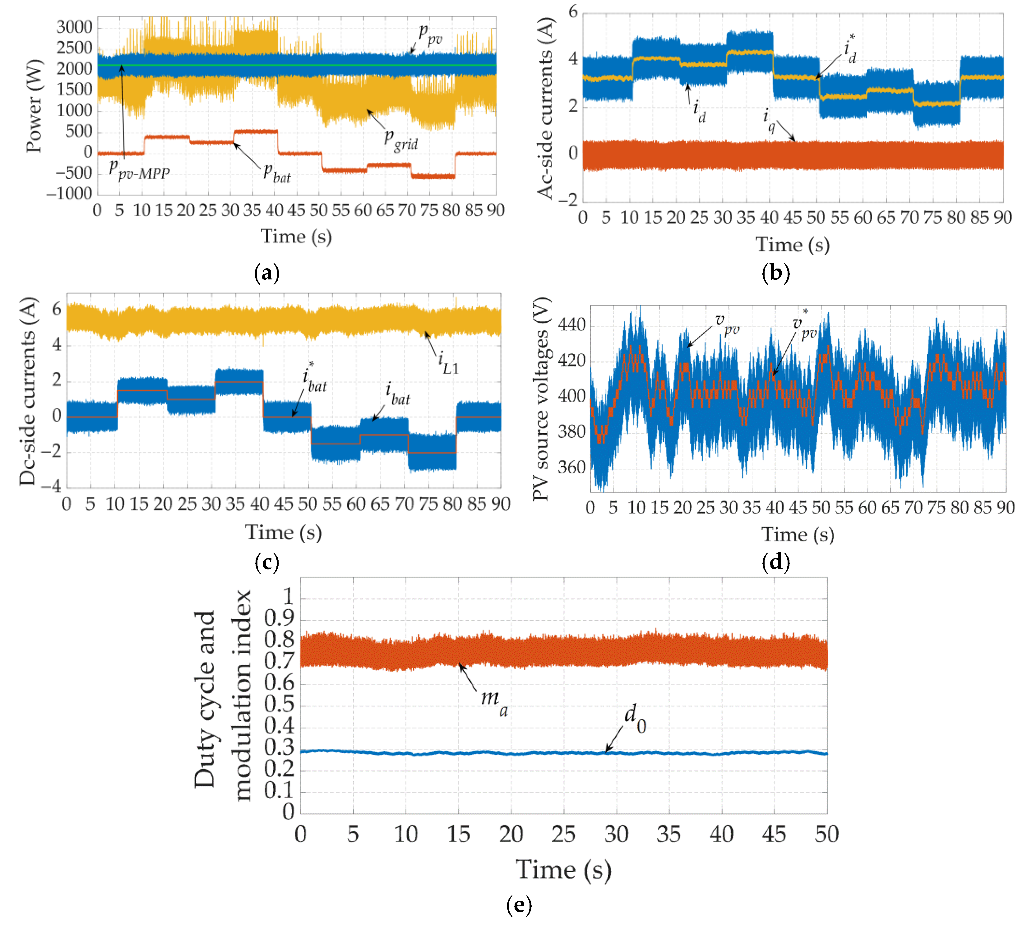
6.2.1. Grid-Tied Operation

Figure 17 shows the waveforms of the system variables in the case of the irradiance variation, with the reference battery current set to zero (i*bat = 0 A). At the beginning, the irradiance (Z) is equal to 600 W/m2 and changes approximately every 10 s in the following order: 300 W/m2, 700 W/m2, 1000 W/m2, 800 W/m2. Figure 17a shows that the decrease in the irradiance causes a decrease in the PV source power. Due to i*bat = 0 A, the battery power is equal to zero, whereas the variation of the grid power follows the variation of the PV source power. The d-axis grid current (id) follows the reference value (i*d), which varies with the irradiance in order to maintain i*bat = 0 A, as shown in Figure 17b. On the other hand, the q-axis grid current is equal to zero, which ensures the unity power factor. Figure 17c shows that the qZSI input current (iL1) follows the irradiance change, whereas the battery current (ibat) stays equal to the reference value of 0 A. The PV source voltage (vpv) follows v*pv, generated by the MPPT algorithm, which decreases with the irradiance, as shown in Figure 17d. Finally, Figure 17e shows the duty cycle (d0) and modulation index (ma), which are practically constant during the experiment due to the fact the vpv variations were marginal.
It may be seen that the proposed MPPT algorithm accurately tracks the maximum available PV power (ppv-MPP) for all the considered irradiance values, with the fast responses to irradiance variations. On the other hand, the battery controller ensures high robustness to disturbances in the system and zero steady-state error. Note that d0 and ma are practically constant during the whole experiment, with the only exception being the transient at t = 11 s, where Z decreases in a step manner from 600 W/m2 to 300 W/m2. This means that the assumptions utilized for determination of transfer function from id to ibat, defined in (17), are justified.
Figure 18 shows the waveforms of the system variables in the case of the reference battery current variation, with Z set to 700 W/m2. At the beginning, i*bat is set to 0 A and then changes approximately every 10 s in the following order: 1.5 A, 1 A, 2 A, 0 A, −1.5 A, −1 A, −2 A, 0 A. Figure 18a shows that pgrid increases with the pbat, whereas ppv is constant and equal to ppv-MPP due to the constant values of Z and Tpv. The battery current follows its reference value and there is no overshoot in the ibat response during the step variations of i*bat, as shown in Figure 18c (similar ibat waveforms may be obtained by the utilization of a simulation model of the battery control loop shown in Figure 3). Figure 18d shows that the PV voltage oscillates around the MPP, which is a feature of all P&O algorithms, but with no adverse impact on the system performance. The modulation index and the duty cycle are practically unaffected by i*bat variations, as shown in Figure 18e.

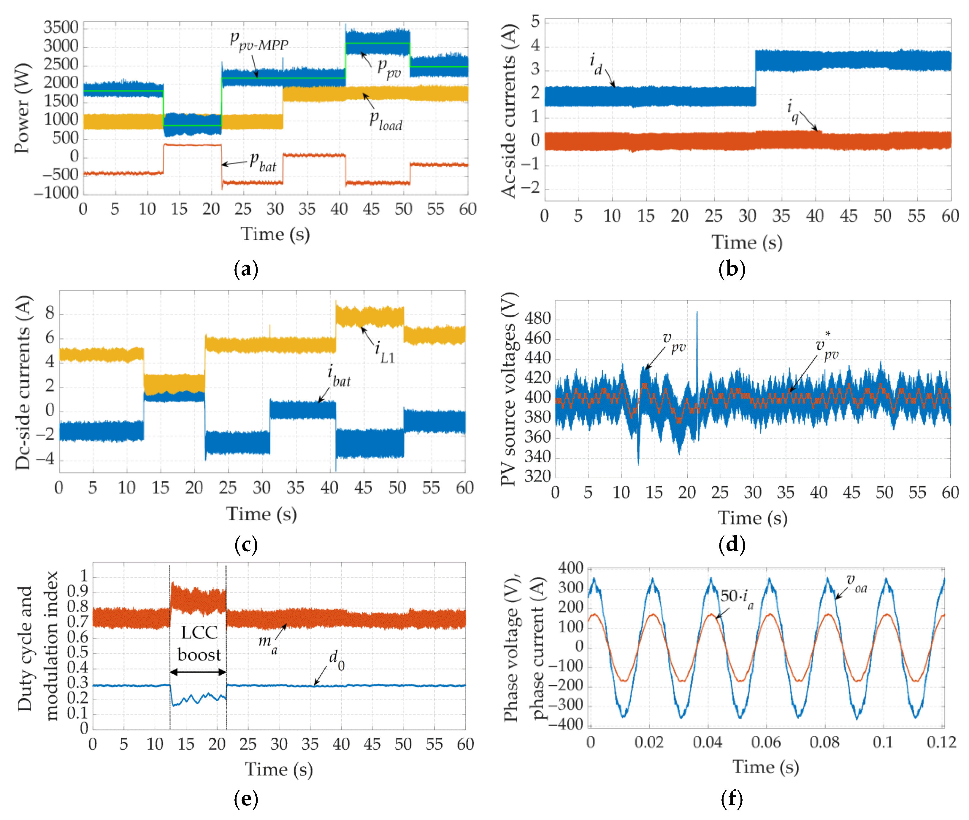
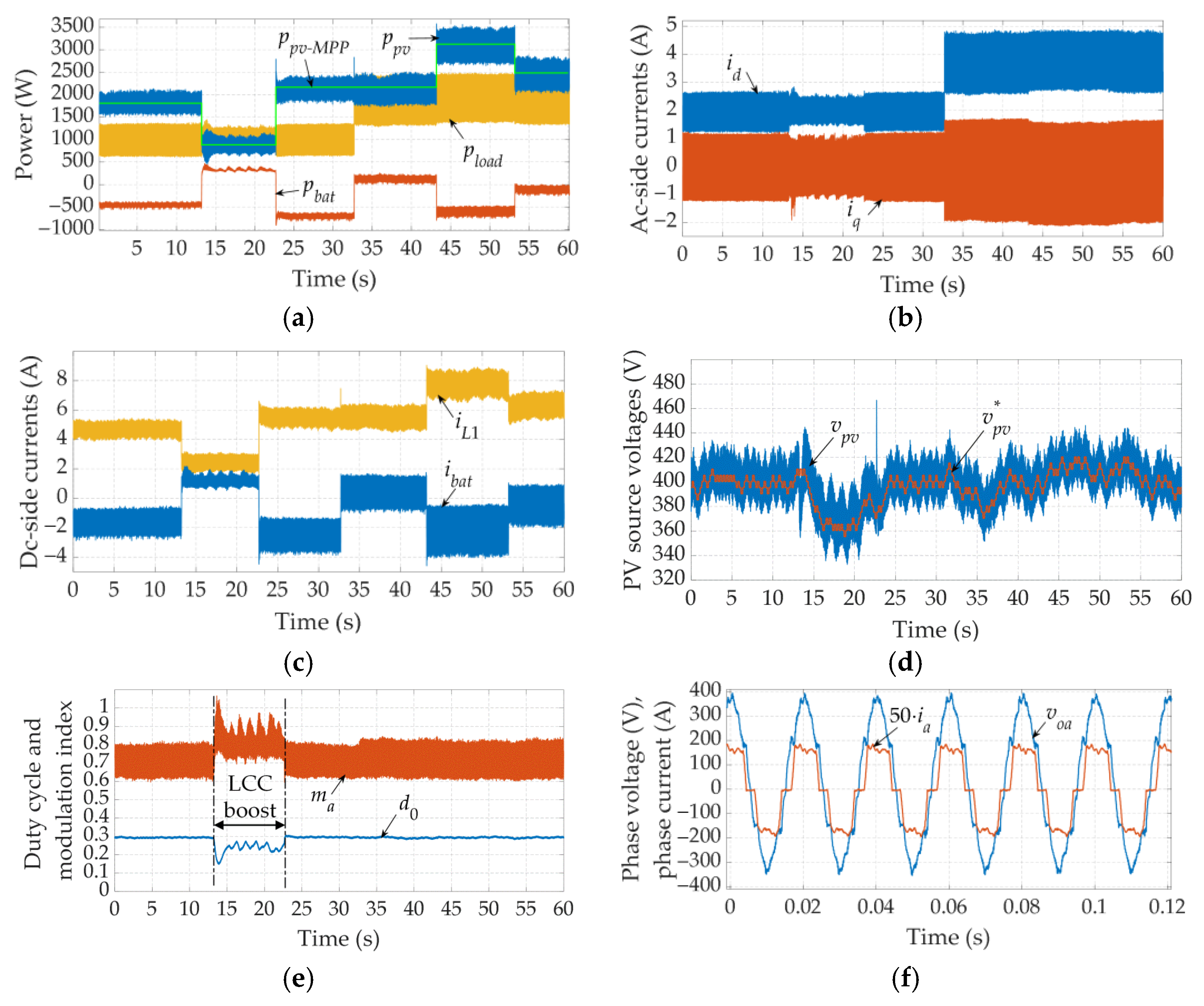
6.2.2. Stand-Alone Operation

Figure 19 shows the responses recorded for the case of the irradiance and load resistance variation with Vl,max set to 340 V in order to ensure approximately the same output voltage level as in the utility grid. At the beginning, Z is equal to 600 W/m2 and it is varied at 12 s, 22 s, 41 s, and 51 s, in the following order: 300 W/m2, 700 W/m2, 1000 W/m2, 800 W/m2, respectively. On the other hand, the load resistance is changed at 32 s from 175 Ω to 90 Ω (i.e., the load power is increased from 990 W to 1926 W). Figure 19a shows that ppv follows ppv-MPP as accurately as during the grid-tied operation and is not affected by the load resistance variation. id increases with the load power with a smooth transient, whereas iq is equal to zero due to the applied pure resistive load, as shown in Figure 19b. The battery current in this operation is not controlled, so it increases with the irradiance decrease. As a result of the decrease in the load resistance, ibat increases to cover the load power requirements.
Note in Figure 19e that, in the case of Z = 300 W/m2, the values of the modulation index and duty cycle are significantly different than in the case of higher irradiances. This is due to the occurrence of the so-called load-caused current (LCC) boost [32,33,34], where the impedance network diode blocks during the non-ST state, which is normally not the case. However, this does not affect the MPPT algorithm, which still achieves tracking of ppv-MPP. In this study, the LCC boost has been detected online as described in Appendix B. Note that all the variables required for the LCC boost detection are already known in the considered control algorithm. Figure 19f shows the phase voltage (voa) and current (ia), which are in this case practically sinusoidal (THD ≈ 4%).
The same experiment as in Figure 19 was performed for the case of the non-linear load, which was composed of the three-phase full-bridge diode rectifier and the resistive load. Figure 20 shows that the system performance was equally as good as in the case of the linear resistive load. Figure 20f shows that voa is slightly more distorted (THD ≈ 7%) despite of the existence of the low-order harmonics in ia. It is assumed that the distortion of the phase currents causes the ripple of id and iq to be higher than in case of the linear load.
Figure 21 shows the waveforms recorded for the case of MBC = 0 and MBC = 1 for different irradiance values and the load resistance value of 175 Ω. At the beginning, MBC = 0, Z = 700 W/m2, and ppv = ppv-MPP, resulting in battery charging of approximately 600 W. At t = 11 s, the batteries are fully charged, MBC changes to 1 and ppv departs from ppv-MPP by increasing v*pv to achieve ibat ≈ 0 A and prevent further charging of the batteries. The length of the respective transient period is approximately 1.5 s. Further, at t = 26 s, the irradiance decreases to 600 W/m2, resulting in a transient period of approximately 2 s. After this transient, the batteries were slightly discharging because of the error related to the Δv*pv value, as described above. At t = 41 s, the irradiance decreases to 300 W/m2 and the battery current becomes positive (discharging) due to the low PV source power. Consequently, ppv is again set equal to ppv-MPP by the control algorithm to achieve minimum discharging current. At t = 56 s, the irradiance increases to 500 W/m2, causing a rapid increase in the PV source power, which results in negative ibat (charging). As a result, the control algorithm increases v*pv to achieve ibat ≈ 0 A, which is accomplished in approximately 2.5 s. Finally, at t = 71 s, MBC becomes 0, allowing the batteries to be charged again. Consequently, v*pv decreases to ensure ppv = ppv-MPP, which is accomplished in approximately 1.5 s.

7. Conclusions

The accuracy of the three derived transfer functions utilized for the control system design was found to be satisfactory, with the maximum steady-state errors of the calculated responses not surpassing 12%. The dynamic transients obtained by the transfer functions from the d-axis current to the battery current and from the duty cycle to the PV source voltage corresponded to measurements with negligible error. This confirmed the accuracy of the proposed small-signal model and allowed these two transfer functions to be utilized for PI controller tuning and the analysis of the system stability. In addition, the settling times of the transients obtained by the transfer function from the duty cycle to the battery current matched well with those obtained experimentally. This allowed the considered transfer function to be utilized for the determination of the tracking period of the MPPT algorithm because the longest settling time of the battery current response is noted for step changes in the duty cycle.
The recorded experimental responses of the system variables to the rapid changes in the irradiance and the reference battery current during the grid-tied operation confirm excellent MPP tracking and stable operation. A maximum settling time of 0.4 s is noted for the abrupt decrease in the PV source power of 1000 W, whereas the static tracking efficiency of the proposed MPPT algorithm ranged from 96.9% to 100%. As for the reference battery current variations, the settling time of all the considered transients amounted to approximately 0.3 s. During the stand-alone operation, the MPP tracking was again excellent and the system responded to the rapid changes in the irradiance as well as during the grid-tied operation. This confirms the validity of the proposed MPPT algorithm, whose utilization reduces system implementation costs due to the elimination of one current sensor compared to the conventional P&O algorithm. During the rapid changes in the load power (both for the linear and the non-linear load), the settling time amounted to approximately 0.2 s. Finally, it was shown that the implementation of the maximum battery charge signal during the stand-alone operation prevents overcharging of the batteries by setting the battery current approximately to zero.

Author Contributions

Conceptualization, I.G., D.V. and M.B. (Mateo Bašić); methodology, I.G. and D.V.; software, I.G. and M.B. (Matija Bubalo); validation, I.G.; formal analysis, I.G. and D.V.; investigation, I.G. and D.V.; resources, D.V.; data curation, I.G.; writing—original draft preparation, I.G.; writing—review and editing, D.V. and M.B. (Mateo Bašić); visualization, I.G.; supervision, D.V.; project administration, D.V.; funding acquisition, D.V. All authors have read and agreed to the published version of the manuscript.

Funding

This work has been fully supported by the Croatian Science Foundation under the project (IP-2016-06-3319).

Institutional Review Board Statement

Not applicable.

Informed Consent Statement

Not applicable.

Data Availability Statement

Not applicable.

Conflicts of Interest

The authors declare no conflict of interest.

Appendix A

Three inductors, all with inductances of 4.32 mH, were available. Two inductors were placed on the inverter side (Lf1 = 8.64 mH), whereas one was placed on the grid side (Lf2 = 4.32 mH). The capacitance Cf was obtained as follows [35]:
C f = 7 100 I n 20 ω V n = 7 100 P n 3 ω V n 2 = 7 100 3000 3 314.159 230 2 4   μ F
In (A1), In and Vn represent RMS phase current and voltage, respectively. Selected Cf ensures the reactive power of filter capacitors not to be higher than 7% of nominal power (Pn) (recommendation 5–10%). In this way, the resonant frequency (fres) of 1200 Hz, calculated in (25), meets the following condition [36]:
10 f < f r e s < f s w / 2
where f represents the fundamental frequency of the output inverter voltage/current (50 Hz in this study), whereas fsw represents the switching frequency (5 kHz in this study).
Finally, the corresponding damping resistance is obtained as follows [37]:
R d = 1 3 1 2 π f r e s C f 10 Ω

Appendix B

The load-caused current (LCC) boost is characterized by the diode in the qZSI impedance network blocking during the non-ST state. Based on the equivalent circuit for the non-ST state, shown in Figure 2a, the LCC boost occurs if the following condition is met:
i p n > i L 1 + i L 2
The occurrence of the LCC boost causes the unintended boost increase. The existence of the PV source voltage controller in this study eliminates the potential adverse effects of the LCC boost.
In the case of the ideal qZSI, with considered sinusoidal output currents, the maximum value of ipn is equal to the peak phase current Iph,max. Figure A1 shows the current of both the impedance network inductors. The LCC boost certainly will not occur if:
I L 1 , m i n + I L 2 , m i n > I p h , m a x
The minimum values of the inductor currents IL1,min, IL2,min are calculated as:
I L 1 , m i n = I L 1 Δ I L 1 2 I L 2 , m i n = I L 2 Δ I L 2 2
Figure A1. Waveforms of the dc-side currents.
Energies 15 00850 g0a1
The current ripples in (A6) are considered equal and may be calculated according to the equivalent circuit for the ST state, shown in Figure 2b, as follows:
Δ I L 1 = Δ I L 2 = V C 1 T 0 2 L
By applying (A6) and (A7), (A5) becomes:
I L 1 + I L 2 V C 1 T 0 2 L > I p h , m a x
By applying IL2 = IL1Ibat and IL1 = Ppv/Vpv, (A5) becomes:
2 P p v V p v I b a t V C 1 T 0 2 L > I p h , m a x
In the case of the ideal qZSI, the following applies:
P p v + P b a t = P o u t P b a t = I b a t V b a t P o u t = 3 V p h , m a x 2 I p h , m a x cos ϕ = 3 4 V p v M a I p h , m a x cos ϕ 1 2 d 0 = 3 8 Z l cos ϕ V p v 2 M a 2 ( 1 2 d 0 ) 2 V C 1 = 1 d 0 1 2 d 0 V p v ; V b a t = d 0 1 2 d 0 V p v
In (A10), capital letters represent the mean values of the considered variables. Vph,max represents the peak phase voltage, whereas Zl represents the equivalent output impedance, which may be obtained as Vph,max/Iph,max. Finally, by applying (A10), (A9) becomes:
3 cos ϕ M a 2 4 Z l ( 1 2 d 0 ) T 0 ( 1 d 0 ) 2 L I b a t V p v > M a 2 2 Z l
Equation (A11) has been utilized for the online detection of the LCC boost during the experimental investigation of the considered system.

References

  1. Bianconi, E.; Calvente, J.; Giral, R.; Mamarelis, E.; Petrone, G.; Ramos-Paja, C.A.; Spagnuolo, G.; Vitelli, M. A fast current-based MPPT technique employing sliding mode control. IEEE Trans. Ind. Electron. 2013, 60, 1168–1178. [Google Scholar] [CrossRef]
  2. Errouissi, R.; Al-Durra, A.; Muyeen, S.M. A robust continuous-time MPC of a DC–DC boost converter interfaced with a grid-connected photovoltaic system. IEEE J. Photovolt. 2016, 6, 1619–1629. [Google Scholar] [CrossRef] [Green Version]
  3. Jain, C.; Singh, B. A three-phase grid tied SPV system with adaptive DC link voltage for CPI voltage variations. IEEE Trans. Sustain. Energy 2016, 7, 337–344. [Google Scholar] [CrossRef]
  4. Anderson, J.; Peng, F.Z. Four quasi-Z-source inverters. In Proceedings of the 2008 IEEE Power Electronics Specialists Conference, Rhodes, Greece, 15–19 June 2008; pp. 2743–2749. [Google Scholar]
  5. Monjo, L.; Sainz, L.; Mesas, J.J.; Pedra, J. State-space model of quasi-z-source inverter-PV systems for transient dynamics studies and network stability assessment. Energies 2021, 14, 4150. [Google Scholar] [CrossRef]
  6. Monjo, L.; Sainz, L.; Mesas, J.J.; Pedra, J. Quasi-Z-source inverter-based photovoltaic power system modeling for grid stability studies. Energies 2021, 14, 508. [Google Scholar] [CrossRef]
  7. Ge, B.; Abu-Rub, H.; Peng, F.Z.; Lei, Q.; Almeida, A.T.d.; Ferreira, F.J.T.E.; Sun, D.; Liu, Y. An energy-stored quasi-z-source inverter for application to photovoltaic power system. IEEE Trans. Ind. Electron. 2013, 60, 4468–4481. [Google Scholar] [CrossRef]
  8. Ge, B.; Peng, F.Z.; Abu-Rub, H.; Ferreira, F.J.T.E.; Almeida, A.T.d. Novel energy stored single-stage photovoltaic power system with constant DC-link peak voltage. IEEE Trans. Sustain. Energy 2014, 5, 28–36. [Google Scholar] [CrossRef]
  9. Abu-Rub, H.; Iqbal, A.; Ahmed, S.M.; Peng, F.Z.; Li, Y.; Baoming, G. Quasi-Z-source inverter-based photovoltaic generation system with maximum power tracking control using ANFIS. IEEE Trans. Sustain. Energy 2013, 4, 11–20. [Google Scholar] [CrossRef]
  10. Grgić, I.; Bašić, M.; Vukadinović, D.; Bubalo, M. Fixed-duty-cycle control of a quasi-z-source inverter in a battery-assisted photovoltaic system. In Proceedings of the 2019 20th International Symposium on Power Electronics (Ee), Novi Sad, Serbia, 23–26 October 2019; pp. 1–6. [Google Scholar]
  11. Khajesalehi, J.; Sheshyekani, K.; Hamzeh, M.; Afjei, E. High-performance hybrid photovoltaic -battery system based on quasi-Z-source inverter: Application in microgrids. IET Gener. Transm. Distrib. 2015, 9, 895–902. [Google Scholar] [CrossRef]
  12. Li, F.; Ge, B.; Sun, D.; Bi, D.; Peng, F.Z.; Haitham, A.R. Quasi-Z source inverter with battery based PV power generation system. In Proceedings of the 2011 International Conference on Electrical Machines and Systems, Beijing, China, 20–23 August 2011; pp. 1–5. [Google Scholar]
  13. Liu, Y.; Ge, B.; Abu-Rub, H.; Iqbal, A.; Peng, F. Modeling and controller design of quasi-Z-Source inverter with battery based photovoltaic power system. In Proceedings of the 2012 IEEE Energy Conversion Congress and Exposition (ECCE), Raleigh, NC, USA, 15–20 September 2012; pp. 3119–3124. [Google Scholar]
  14. Liu, Y.; Ge, B.; Abu-Rub, H.; Peng, F.Z. Control system design of battery-assisted quasi-z-source inverter for grid-tie photovoltaic power generation. IEEE Trans. Sustain. Energy 2013, 4, 994–1001. [Google Scholar] [CrossRef]
  15. Liu, Y.; Ge, B.; Abu-Rub, H.; Peng, F.Z. Modelling and controller design of quasi-Z-source inverter with battery-based photovoltaic power system. IET Power Electron. 2014, 7, 1665–1674. [Google Scholar] [CrossRef]
  16. Sun, D.; Ge, B.; Bi, D.; Peng, F.Z. Analysis and control of quasi-Z source inverter with battery for grid-connected PV system. Int. J. Electr. Power Energy Syst. 2013, 46, 234–240. [Google Scholar] [CrossRef]
  17. Sun, D.; Ge, B.; Peng, F.Z.; Rub, H.A.; Almeida, A.T.D. Power flow control for quasi-Z source inverter with battery based PV power generation system. In Proceedings of the 2011 IEEE Energy Conversion Congress and Exposition, Phoenix, AZ, USA, 17–22 September 2011; pp. 1051–1056. [Google Scholar]
  18. De Oliveira-Assis, L.; Soares-Ramos, E.P.P.; Sarrias-Mena, R.; García-Triviño, P.; González-Rivera, E.; Sánchez-Sainz, H.; Llorens-Iborra, F.; Fernández-Ramírez, L.M. Simplified model of battery energy-stored quasi-Z-source inverter-based photovoltaic power plant with Twofold energy management system. Energy 2021, 122563. [Google Scholar] [CrossRef]
  19. Babaa, S.E.; Armstrong, M.; Pickert, V. Overview of maximum power point tracking control methods for PV systems. J. Power Energy Eng. 2014, 2, 59–72. [Google Scholar] [CrossRef] [Green Version]
  20. Eltawil, M.A.; Zhao, Z. MPPT techniques for photovoltaic applications. Renew. Sustain. Energy Rev. 2013, 25, 793–813. [Google Scholar] [CrossRef]
  21. Tofoli, F.L.; de Castro Pereira, D.; de Paula, W.J. Comparative study of maximum power point tracking techniques for photovoltaic systems. Int. J. Photoenergy 2015, 2015, 812582. [Google Scholar] [CrossRef]
  22. Yazdani, A.; Iravani, R. Voltage-Sourced Converters in Power Systems: Modeling, Control, and Applications; John Wiley & Sons: Hoboken, NJ, USA, 2010. [Google Scholar]
  23. Dannehl, J.; Wessels, C.; Fuchs, F.W. Limitations of voltage-oriented pi current control of grid-connected PWM rectifiers with LCL filters. IEEE Trans. Ind. Electron. 2009, 56, 380–388. [Google Scholar] [CrossRef]
  24. Grgić, I.; Vukadinović, D.; Bašić, M.; Bubalo, M. Efficiency boost of a quasi-z-source inverter: A novel shoot-through injection method with dead-time. Energies 2021, 14, 4216. [Google Scholar] [CrossRef]
  25. LEM. Current Transducer LA 55-P/SP52. Available online: https://www.lem.com/sites/default/files/products_datasheets/la_55-p_sp52.pdf (accessed on 12 December 2021).
  26. LEM. Voltage Transducer DVL 500. Available online: https://www.lem.com/sites/default/files/products_datasheets/dvl_500.pdf (accessed on 12 December 2021).
  27. LEM. Voltage Transducer CV 3-500. Available online: https://www.lem.com/sites/default/files/products_datasheets/cv_3-500.pdf (accessed on 12 December 2021).
  28. Golestan, S.; Guerrero, J.M.; Vasquez, J.C. Three-phase PLLs: A review of recent advances. IEEE Trans. Power Electron. 2017, 32, 1894–1907. [Google Scholar] [CrossRef] [Green Version]
  29. Vukadinović, D.; Nguyen, T.D.; Nguyen, C.H.; Vu, N.L.; Bašić, M.; Grgić, I. Hedge-algebra-based phase-locked loop for distorted utility conditions. J. Control. Sci. Eng. 2019, 2019, 3590527. [Google Scholar] [CrossRef]
  30. Bollipo, R.B.; Mikkili, S.; Bonthagorla, P.K. Hybrid, optimal, intelligent and classical PV MPPT techniques: A review. CSEE J. Power Energy Syst. 2021, 7, 9–33. [Google Scholar] [CrossRef]
  31. Hohm, D.P.; Ropp, M.E. Comparative study of maximum power point tracking algorithms. Prog. Photovolt. Res. Appl. 2003, 11, 47–62. [Google Scholar] [CrossRef]
  32. Shen, M.; Peng, F.Z. Operation modes and characteristics of the z-source inverter with small inductance or low power factor. IEEE Trans. Ind. Electron. 2008, 55, 89–96. [Google Scholar] [CrossRef]
  33. Liske, A.; Clos, G.; Braun, M. Analysis and modeling of the quasi-Z-source-inverter. In Proceedings of the IECON 2011—37th Annual Conference of the IEEE Industrial Electronics Society, Melbourne, VIC, Australia, 7–10 November 2011; pp. 1197–1202. [Google Scholar]
  34. Kayiranga, T.; Li, H.; Lin, X.; Shi, Y.; Li, H. Abnormal operation state analysis and control of asymmetric impedance network-based quasi-z-source PV inverter (AIN-qZSI). IEEE Trans. Power Electron. 2016, 31, 7642–7650. [Google Scholar] [CrossRef]
  35. Vukosavic, S.N. Grid-Side Converters Control and Design, 1st ed.; Springer: Cham, Switzerland, 2018. [Google Scholar] [CrossRef]
  36. Wei, X.; Xiao, L.; Yao, Z.; Gong, C. Design of LCL filter for wind power inverter. In Proceedings of the 2010 World Non-Grid-Connected Wind Power and Energy Conference, Nanjing, China, 5–7 November 2010; pp. 1–6. [Google Scholar]
  37. Liserre, M.; Blaabjerg, F.; Hansen, S. Design and control of an LCL-filter-based three-phase active rectifier. IEEE Trans. Ind. Appl. 2005, 41, 1281–1291. [Google Scholar] [CrossRef]
Figure 1. Configuration of the considered system PV system with the qZSI and batteries (a), and the logic diagram of the zero-sync PWM (b).
Energies 15 00850 g001
Figure 2. Equivalent circuits of the qZSI: non-ST state (a) and ST state (b).
Energies 15 00850 g002
Figure 3. Battery current control loop.
Energies 15 00850 g003
Figure 4. Control loop of the d-axis load voltage.
Energies 15 00850 g004
Figure 5. Control loop of the PV source voltage.
Energies 15 00850 g005
Figure 6. Grid-tied operation: PV source power, grid power and d-axis current, and battery power (a), and flow chart of the MPPT algorithm (b).
Energies 15 00850 g006
Figure 7. Stand-alone operation: PV source power, load power, and battery power and current (a), and flow chart of the PV source reference voltage determination (b).
Energies 15 00850 g007
Figure 8. Laboratory setup of the qZSI with the PV source and batteries.
Energies 15 00850 g008
Figure 9. Setups utilized for the accuracy verification of transfer functions: from d-axis gird current to battery current (a), and from duty cycle to battery current/ PV source voltage (b).
Energies 15 00850 g009
Figure 10. Waveforms of the battery current obtained by the transfer function and by measurement during transients for: Z = 600 W/m2, Tpv = 30 °C (linearization point) (a), Z = 1000 W/m2, Tpv = 10 °C (b), and Z = 500 W/m2, Tpv = 50 °C (c).
Energies 15 00850 g010
Figure 11. Waveforms of the PV voltage obtained by the transfer function and by measurement during transients for: Z = 600 W/m2, Tpv = 30 °C (linearization point) (a), Z = 600 W/m2, Tpv = 10 °C (b), and Z = 600 W/m2, Tpv = 50 °C (c).
Energies 15 00850 g011
Figure 12. Waveforms of the battery current obtained by the transfer function and by measurement during transients for: Z = 600 W/m2, Tpv = 30 °C (linearization point) (a), Z = 600 W/m2, Tpv = 10 °C (b), and Z = 600 W/m2, Tpv = 50 °C (c).
Energies 15 00850 g012
Figure 13. Bode plot of the battery control loop.
Energies 15 00850 g013
Figure 14. Bode plot of the d-axis voltage control loop.
Energies 15 00850 g014
Figure 15. Bode plot of the PV source voltage control loop.
Energies 15 00850 g015
Figure 16. Steady-state characteristics of the considered system: dc-side powers (a), efficiency (b), d-axis current (c), THD of phase current (d), and input voltage of inverter bridge (e).
Energies 15 00850 g016
Figure 17. Irradiance variation during the grid-tied operation: system powers (a), output grid currents (b), dc-side currents (c), PV source voltage (d), and modulation index and duty cycle (e).
Energies 15 00850 g017
Figure 18. Reference battery current variation during the grid-tied operation: system powers (a), output grid currents (b), dc-side currents (c), PV source voltage (d), and modulation index and duty cycle (e).
Energies 15 00850 g018
Figure 19. Irradiance variation and load resistance variation during the stand-alone operation: system powers (a), output load currents (b), dc-side currents (c), PV source voltage (d), modulation index and duty cycle (e), and phase voltage and current (f).
Energies 15 00850 g019
Figure 20. Irradiance variation and non-linear load resistance variation during the stand-alone operation: system powers (a), output load currents (b), dc-side currents (c), PV source voltage (d), modulation index and duty cycle (e), and phase voltage and current (f).
Energies 15 00850 g020
Figure 21. Irradiance variation and maximum battery charge signal variation during the stand-alone operation: system powers (a), output load currents (b), dc-side currents (c), PV source voltage (d), and modulation index and duty cycle (e).
Energies 15 00850 g021
Table 1. The input parameters of the transfer function from id to ibat.
Rbat (Ω)Rfn (Ω)RL (Ω)Ibat (A)IL1 (A)D0V0bat (V)VC1 (V)Ma
0.7870.504.50.2842686790.72
Table 2. The input parameters of the transfer functions from d0 to ibat and from d0 to vpv.
Rbat (Ω)Rfn (Ω)RL (Ω)Ibat (A)IL1 (A)D0V0bat (V)VC1 (V)Ma
0.7870.51.154.50.2832706720.73
Table 3. The static tracking efficiency of the proposed P&O algorithm.
Z (W/m2)3004005006007008009001000
STE50°C (%)96.997.299.2398.4498.9499.5399.599.63
STE10°C (%)98.8198.9299.8710010099.8199.999.72
Publisher’s Note: MDPI stays neutral with regard to jurisdictional claims in published maps and institutional affiliations.

