Article

Estimating the Pre-Historical Volcanic Eruption in the Hantangang River Volcanic Field: Experimental and Simulation Study

1
Department of Science Education, Kangwon National University, Chuncheon-si 24341, Gangwon-do, Korea
2
Department of Smart Regional Innovation, Kangwon National University, Chuncheon-si 24341, Gangwon-do, Korea
3
Department of Geology, Kangwon National University, Chuncheon-si 24341, Gangwon-do, Korea
*
Author to whom correspondence should be addressed.
Remote Sens. 2022, 14(4), 894; https://doi.org/10.3390/rs14040894
Submission received: 6 January 2022 / Revised: 10 February 2022 / Accepted: 10 February 2022 / Published: 13 February 2022

Abstract

:
The volcanic landforms associated with fluvial topography in the Hantangang River Volcanic Field (HRVF) have geoheritage value. The Hantangang basalt geological landform stretches along 110 km of the paleoriver channel of the Hantangang River. Since the eruption that formed this basalt occurred from 0.15 to 0.51 Ma, estimating the eruption in the HRVF that originated from two source vents in North Korea (Orisan Mountain and the 680 m peak) is challenging due to the limited recorded data for this eruption. In this study, we estimated this prehistorical eruption using 3D printing of a terrain model and Q-LavHA simulation. The results from the experiment were further analyzed using findings from an artificial neural network (ANN) and support vector machine (SVM) to classify the experimental lava area. The SVM classification results showed higher accuracy and efficiency in the computational process than the ANN algorithm. Results from the single eruptive vent scenario showed that the experiment had a higher accuracy than the Q-LavHA simulation. Further analysis of multiple vent scenarios in the Q-LavHA simulation has improved the accuracy compared with the single eruptive vent scenarios.

1. Introduction

The volcanic activity that produces lava flows is known as the effusive eruption type, and this explosive type produces fragmented material, such as pyroclastic flows [1]. The sizes or scales of explosive volcanic eruptions are determined by the volcanic explosion index (VEI) [2]. The VEI measures the erupted volume and eruption plume column height on a scale of 0 to 8 [3]. The largest volcanic eruption with a VEI of 8 occurred on Younger Toba Tuff, Indonesia, with a magnitude of 8.8 at ca. 0.074 Ma [4]; this eruption catastrophically impacted the climate via the ash and sulfate injection into the stratosphere up to more than 100 km from the volcano [5]. The effusive eruption type was measured based on the scale of the eruption by the lava effusion rate [6]. Harris et al. (2007) defined the lava effusion rate as the volume of the ejected lava over a particular time [6]. The highest effusive-type eruption in recorded history occurred from Laki volcano, Iceland. The basaltic lava was discharged with an effusion rate of approximately 5000 m3/s. The eruption began on 8 June 1783 and lasted until 7 February 1784 (8 months long) [7]. Basaltic lava eruptions with high effusion rates and low viscosities can reach more than 100 km in length [8]. Considerable eruption rates up to 107 m3/s within a short period can produce lava widths greater than 100 km; this eruption produced flood basalt flows [9].
This eruption was most probably fed from two vents in the central part of the Korean Peninsula, called the Hantangang River Volcanic Field (HRVF) [10,11,12,13,14] (Figure 1a). The basaltic lava erupted from the two probable source vents of Orisan Mountain and the 680 m peak in Pyeonggang, Gangwon Province, DPRK (Democratic People’s Republic of Korea; North Korea) [10,11], and it flowed down approximately 110 km along the prehistoric Hantangang River channel in Cheor-won-gun, Pocheon-si, and Yeoncheon-gun to Yulgok-ri in Gyeonggi Province, ROK (Republic of Korea; South Korea) [14]. The eruption’s impact on the geological structure has caused the Hantangang River area to be designated by The United Nations Educational, Scientific, and Cultural Organization (UNESCO) as a geopark that can sustainably preserve geological heritage. [15]. A preliminary study of prehistoric basaltic eruptions was carried out via experiments and simulations to infer the possible eruption events that formed the HRVF and the geological heritage values.
The volcanic eruption experiments were conducted using 3D printed materials to study the lava flow from the two source vents in the Korean Peninsula. The use of 3D printed materials has been employed to study geoscience [16], mining [17], earthquakes [18], floods [19], and landslides [20]. The recent application of 3D printing has also created a 3D digital terrain model for educational and research purposes [21]. The digital elevation model reconstruction over an area using the 3D printing method has proven useful for documenting natural heritage sites for spatial planning and education [22]. Therefore, the geoheritage value of the Hantangang River Geopark can be visualized, and the experimental eruption process can become a natural heritage document for educational and research purposes. An image of experimental eruptions from the 3D terrain model was further processed using supervised classification to identify the experimental lava and non-lava area based on the rule of binary classification [23].
The supervised classification method was developed using different techniques, such as the statistics learning method (naïve Bayes and Bayesian networks), logical learning method (decision trees and random forest), support vector machine (SVM), and artificial neural network (ANN). Between those methods, SVM and ANN tend to show better performances in dealing with the continuous features in multi-dimensional data [24]. Thus, in the imbalanced data cases, the SVM and ANN could minimize the overall error rate during the learning process [25]. In its basic form, SVM as a binary classifier was appropriate for use in this study to classify the two classes of area, consisting of the experimental lava area and non-lava area between the decision boundary of a hyperplane [26,27]. Meanwhile, the ANN attempts to mimic the neurons in the human brain [28]. ANN could perform a binary classification using a single hidden layer for modeling nonlinear function [29,30]. ANN performed better than random forest in numerical prediction due to the neural network construction, which has higher performance potential [31,32]. The advantage of SVM and ANN for classification is that SVM works well in classification with the help of a kernel as a classifier and ANN works well for classification by using a single hidden layer for binary classification. Those advantages could reduce the time consumption for the classification process compared with the random forest, which has a disadvantage that time consumption for classification is dependent on the number of input datasets [33].
We utilized an artificial neural network (ANN) and a support vector machine (SVM) as the classifier algorithms, which have been widely suggested in many studies to have high performance accuracy [34,35,36,37]. ANNs and SVMs are widely used to classify aerial photography from drone images of pine wilt disease [35]; Landsat-8 and Sentinel-2 satellite images of postearthquake damage in Palu, Central Sulawesi, and Indonesia [38]; Landsat-8 images of volcanic ashfall and pyroclastic material mapping in Mount Agung, Sinabung, and Merapi, Indonesia [37,39]; postwildfire burned Sokcho Wildfire areas in South Korea [36]; and Landsat images used to classify land cover on a volcanic island in the Aleutian Arc [34]. These studies showed that both algorithms are comparable for classification, with ANNs having better accuracy than SVMs for pyroclastic material and volcanic ashfall classification [37,39]. Moreover, the SVM was better for classifying drone imagery [37] and postdisaster damage mapping of earthquakes [38] and wildfires [36,40]. Nevertheless, neither method has been applied to classify the volcanic processes simulated on a 3D-printed terrain model based on a vertical photograph. The utilization of both classification methods was one of the objectives of this study.
The simulation of the volcanic eruption was also conducted using the computational processing of the Q-LavHA plugin. Q-LavHA has been widely used to simulate historical lava flows, develop hazard inundation maps, and support crisis management [41]. Several volcanic eruptions, such as Mount Etna (Italy), Nyamuragira Volcano (D.R. Congo) [41], Paricutin Volcano (Michoacán, México) [42], Montaña de Aguarijo, El Hierro (Canary Islands, Spain) [43], Karthala Volcano, and Grande Comore Island, were simulated using Q-LavHA [44]. The application of Q-LavHA helped assess the lava flow emplacement based on a digital elevation model (DEM) of volcanic hazard assessment and study historical volcanic eruptions. Thus, the prehistorical eruption on Orisan Mountain, as the origin of the Hantangang River Volcanic Field, was simulated through the Q-LavHA plugin in Quantum Geographical Information System (QGIS) software based on the DEM from Shuttle Radar Topography Mission (SRTM) 1 Arc-Second Global. The vent location and eruption type were discussed to find the best fit with the Quaternary volcanic field as the real lava flow from geological surveys in the Hantangang River [14]. The models were used to generate the probability of a lava flow using a kinematic thermorheological model for lava flowing in a channel (FLOWGO). A sensitivity analysis was conducted to assess the quality of the lava flow simulation compared to that of a real lava flow.
The objective of this study was to implement a digital terrain model based on a 3D printing application for simulating prehistorical volcanic eruptions. The 3D printing approach to simulate natural disaster phenomena that occur on the Earth’s surface was applied to solve the common misconceptions about the earthquake by utilizing a 3D-printed fault model of California faults [18]. Another study also implemented 3D printing of a terrain model to visualize the flooding process caused by the Xiaojiaqiao barrier lake dam break [19]. Digital terrain 3D printing was also used to reconstruct the natural heritage [22], perform lunar and planetary terrain analysis [21] and model the cityscapes for urban visualization [45]. To date, 3D printing has not yet been applied to understand the volcanic processes of the prehistorical eruption that created the natural heritage site. Additionally, in recent years, the Q-LavHA simulation [41] has been applied to understand historical lava flows [42,43,44,46]. The ability of Q-LavHA to forecast the lava flow has not yet been applied in the case of a prehistorical volcano with limited eruption data and may be a challenge of this study. Therefore, the results from the Q-LavHA simulation and the classification of the 3D printing simulation were compared with ground truth data from the geologic map of the HRVF [14].

2. Materials and Methods
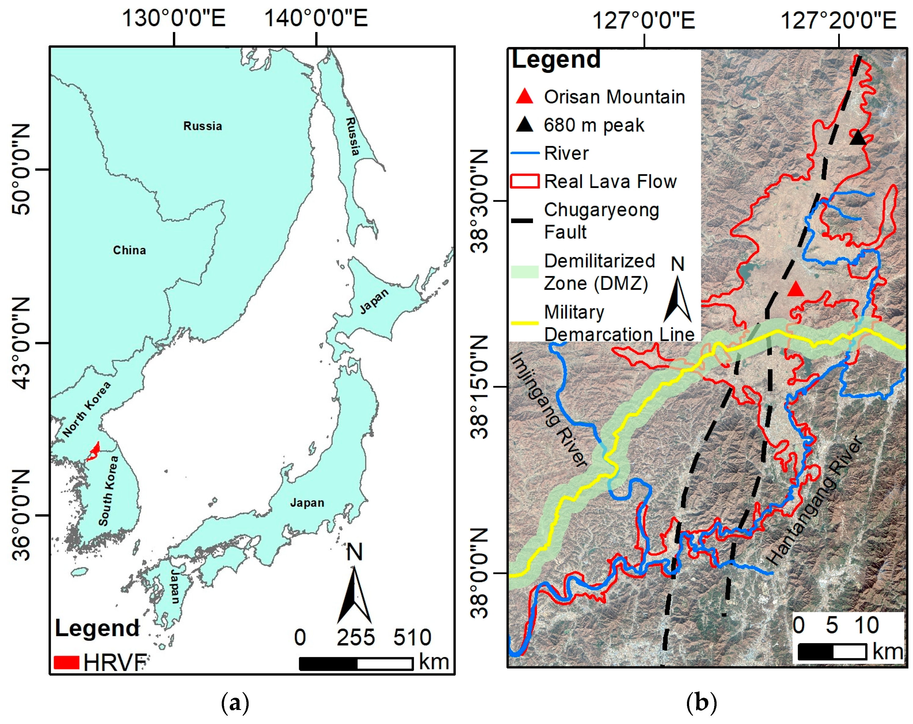
2.1. Study Area

The study area extends between the coordinates of 37°53′28.07″~38°42′18.27″ N and 126°48′42.64″~127°25′58.16″ E near the boundary of North Korea and South Korea (Figure 1b). The average annual temperature of the HRVF is approximately 10.2 °C, with precipitation of approximately 1400 mm during summer seasons [14]. Orisan Mountain, known as one of the possible vents of the HRVF, has an elevation of 444 m above sea level with a gentle slope and shows plains elevation due to lava overflows during the prehistoric eruption. The 680 m peak in North Korea, which is the other vent, has an elevation of 680 m above sea level. Field data on the vents are not available due to restricted access to North Korea. Hence, they are evaluated as possible vents of the HRVF by only topography and aerial photographs [11]. The Hantangang River became a UNESCO Global Geopark due to the unique volcanic topography created by continuous fluvial erosion that cuts through a deep gorge on a flat plateau (https://en.unesco.org/, accessed on 3 February 2022).
The HRVF area consists of Precambrian and Paleozoic metamorphic rocks, Jurassic and Cretaceous granites, Cretaceous volcanic rocks, and Quaternary basalts [10,11,12,13,14,47,48]. The volcanic sources of the HRVF are aligned along the Chugaryeong Fault in the central Korean Peninsula, and the basaltic lava is presumed to have erupted through the fault by fissure eruption [47,49]. The Chugaryeong Fault is located between Wonsan (North Korea) and Seoul, has a direction of NNE to SSW [10,12], and has been evaluated as a strike-slip fault that formed with the volcanic activity of the HRVF in the Quaternary period [50].
In the upstream Hantangang River, eleven basaltic lava flow units have been recognized, and in the downstream area (Jeongok area), the number of lava flow units decreases to 3 or 4, with a thickness of less than 4 m [11]. Nagaoka et al. (2008) subdivided the Quaternary basalt distributed in the Jeongok area into two stratigraphic units based on the existence of erosive valleys and soil between the units: the Jeongok basalt (lower), which is composed of at least three flow units, and the Chatan basalt (upper), which is composed of at least seven flow units [51]. Ryu et al. (2011) suggested that the weighted average ages (eruption ages) of both basalts by K-Ar dating are 0.15 ± 0.01 Ma and 0.51 ± 0.01 Ma, with a time gap of 360,000 years [13]. There are no recorded data on the effusion rate and volume parameter of the series of basaltic lava flows that have erupted in the HRVF. However, it is evident that the thinness of basaltic lavas in the HRVF gradually decreases from 71 m in Cheorwon-gun to 2 or 3 m in Yulgok-ri, which indicates that the flow direction of the basaltic lavas from the possible vents in North Korea is southwestward after eruption [14].
The lava flows of the HRVF are alkali basalts based on the geochemical characteristics of the major elements, which are similar to other Quaternary volcanic rocks in Korea [11,14]. Sr and Nd isotopic compositions reveal that intraplate volcanic activity formed the HRVF [11]. Low contents of SiO2, Na2O, and K2O made the lava flows highly mobile, resulting in a flat lava plateau extending ca. 110 km from the sources in the area [14].

2.2. 3D Model Preparation

The model preparation was initiated by utilizing the digital elevation model (DEM) from the Shuttle Radar Topography Mission (SRTM) with one arcsec or 30-m resolution around the study area [52,53]. The SRTM was launched on 11 February 2000 to generate the digital elevation data of most of Earth’s surface between 60° N and 57° S latitude by exploiting C- and X-band interferometers [54,55]. The accuracy of the SRTM DEM was assessed, and the accuracy results indicated high quality with fewer void data [56,57]. The 3D terrain model of the DEM SRTM was produced using the DEMto3D plugin in QGIS [45]. Following cartographic principles, the 3D model was generated using a 1:150,000 scale [58]. The final output print model dimensions are 540 × 360 mm (Figure 2a) with 1.5 vertical exaggerations to enhance surface details and make some low-relief landforms more suitable for printing [16,59,60]. As these dimensions exceeded the maximum build plate of the printer, we divided the model into six parts with dimensions of 18 cm × 18 cm for each part (Figure 2b). The raw printouts required postprocessing. Firstly, we glued all the parts together and placed them on a dedicated base to make the height of the model 6 cm from the ground. In addition, we colored the model based on the interpretation from the Sentinel-2 Satellite and Google Earth imagery using a colorless acrylic primer to make it smooth and water-resistant.

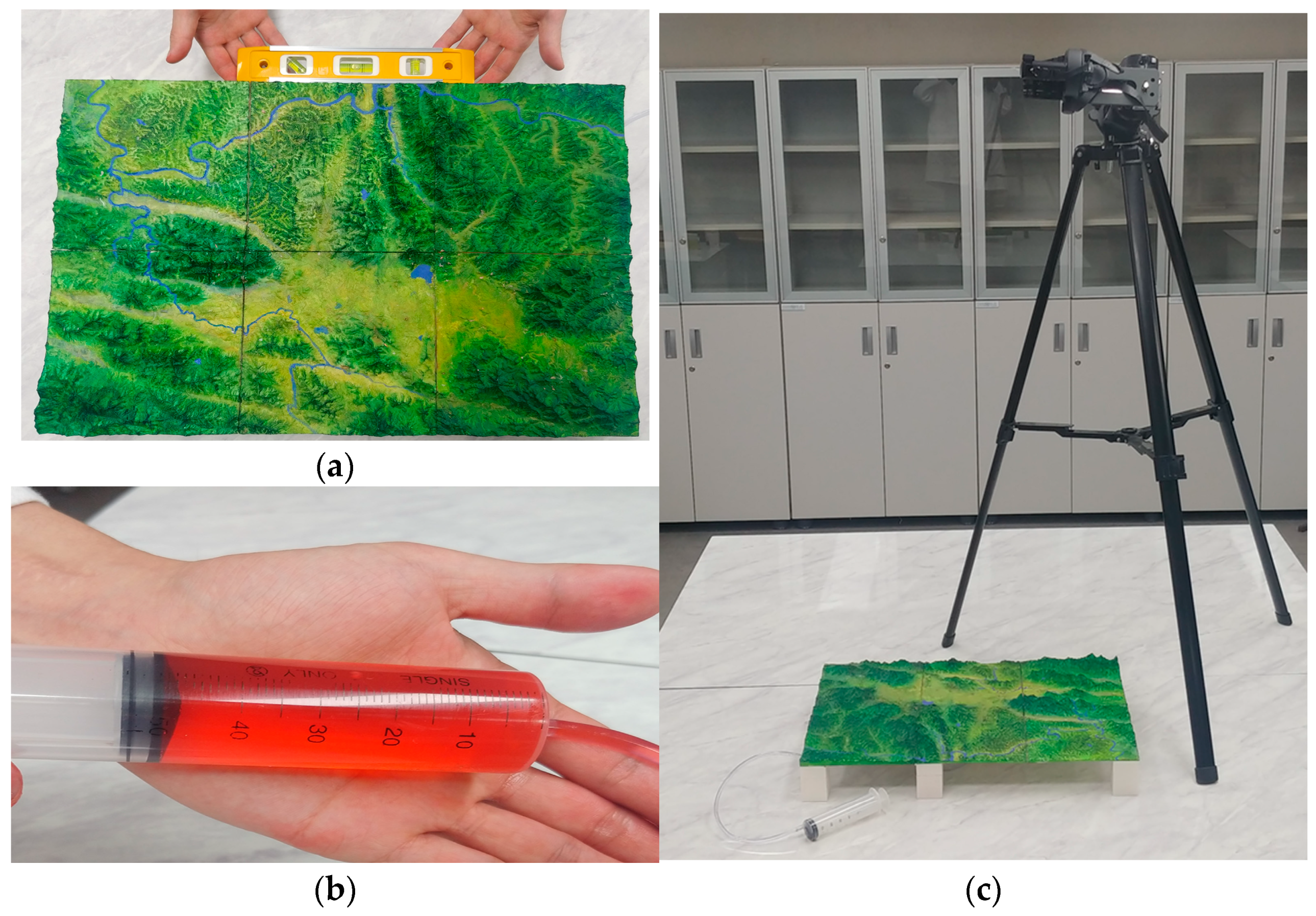
2.3. Experimental Preparation

The materials for the 3D experimental model were ethyl alcohol, red ink, syringes, tube, a tube splitter, a 3D-printed model of approximately the 680 m peak and the Orisan Mountain, a thermohygrometer, and bubble levels (Figure 3a). Ethyl alcohol or ethanol was used as the simulated lava material to avoid surface tension from water that caused clumps on the model. The experiment was conducted at a temperature of approximately 19.6 °C with 40.5% RH (relative humidity). The 3D model was constructed based on the DEM SRTM with a resolution of 30 m, printed on the 3D terrain model, and colored with the Sentinel-2 satellite and Google Earth imageries (Figure 3b). The model was raised approximately 6 cm for installation, with the simulated lava source using a transparent PVC tube as the connector and a syringe as the simulated magma chamber. Needles were inserted at the locations of Orisan Mountain and the 680 m peak (Figure 3c).
The experiment was initiated by stabilizing the surface level of the 3D printed model using the bubble level and aligning the 3D model with the surface level for an accurate experiment (Figure 4a). Before ejecting the simulated lava flow, ethanol was mixed with red ink to visualize the simulated lava flow. The initial condition of the syringe volume was 50 mL with the tube connector under the 3D model filled with red ethanol (Figure 4b). The two experiments were conducted by pushing the syringe at a constant speed to inject the mixed solution from the single eruptive vent, which was Orisan Mountain for the first experiment and the 680 m peak for the second experiment. The experiment was captured and recorded using a camera from the top of the model with the composition of the experimental shoot, as shown in Figure 4c.

2.4. Artificial Neural Network

ANNs are networks consisting of an arbitrary number of elementary elements, called neurons, connected to other neurons [24]. The activation function intensifies or weakens the signal transmitted to other neurons [61]. The single-layer perceptron is the simplest form of neural network and consists of an input layer connected directly with a layer of output neurons. The single-layer perceptron is usually used for binary input data [28]. The multilayer perceptron of a neural network is appropriate for approximating an unknown function, called a hidden layer, between the input and output layers [62]. The multilayer perceptron has the ability for weight adjustment during the training process [63]. The activation function in an ANN controls an input signal, which is produced as an output signal at a certain threshold. Logistic functions are popular due to the simple calculation and comparison with other functions [61,63]. One hidden layer is technically required to perform smooth nonlinear transformation [63]. The parameters of the ANN in this study were set to 0.1, 0.2, and 0.9 for root mean square (RMS) errors at which the training should stop, training rate, and training momentum, respectively. Finally, the number of training iterations was set to 100 to optimize the computational process [35,36,39].

2.5. Support Vector Machine

The support vector machine or SVM is a supervised machine learning algorithm that can separate the dataset that is consistent with the training samples through the decision boundary at the hyperplane [64]. The ability of SVM as a linear binary classifier in its simplest form that can handle small training datasets was suitable for use in this study to separate the individual pixel between the simulated lava flow area and the area with no simulated lava flow from the experimental result [27]. The learning process of the SVM algorithm was based on structural risk minimization that is capable of maximizing the margin width of the decision boundary and minimizing the classification error without any assumption [35,65]. Selecting a suitable kernel for operating SVM machine learning for the classification process can reduce the computational process [66]. The radial basis function (RBF) kernel is the most popular kernel and is often used for SVMs due to its ability to perform excellently in nonlinear classification problems [34,35,36,38,67]. The parameter options that control the possibility of higher accuracy for classification results, such as penalty parameter c and gamma γ , were set to 100 and 0.5, respectively. The zero value was set into the pyramid parameter and classification probability threshold value to process the input image in full resolution and to assign the class label for all pixels of the input image [36,38].

2.6. Q-LavHA Simulation

The simulation of the lava flow was conducted by the Q-LavHA plugin that was integrated into the QGIS software. The model simulates the lava from single or multiple eruptive vents on a digital elevation model (DEM). Q-LavHA integrated three alternative models to terminate the simulated lava flow. The first two models ( L max ) and ( L normal ) simulated lava flow based on the probabilistic approach. L max defines the maximum length of the lava based on the distance covered by the flow [68], while L normal defines the maximum length of lava flow from the mean and the standard deviation of historical lava flows using a decreasing cumulative distribution function [41]. These two models were easy and fast in simulating lava flows by only utilizing the maximum length reached by the historical lava flow. The uncertainty of the time interval and ejection lava volume in each effusive episode means that the simulation is based on the maximum length of the present lava flow vague. Another lava flow simulation method ( L flowgo ) relies on thermorheological parameters to control the lava flows to be stopped at a certain point until the velocity of the lava reaches zero [69].
The Q-LavHA simulation, based on the L flowgo method, was used in this study by utilizing the parameters presented in Table 1. These parameters determine the lava flow speed and trajectory [43]. The basic principle of Q-LavHA is that the simulated lava propagates through the surrounding elevation pixels in the DEM [41]. The existence of a sink or depression in the DEM could halt the simulated lava flows. The DEM error is solved by filling the sinks in a surface raster to remove the imperfection of the DEM, such as local holes or sinks [42]. The accuracy of the simulated lava flow is analyzed by comparing it with the real lava flow from geological data [42,46,70,71]. Another method to assess the real lava flow is by reconstructing the topography and morphology from the past eruption by fieldwork [43]. In this study area, fieldwork cannot be carried out due to the political situation, so the best way to compare the simulated lava flow in this study was using the geological map constructed by Kil et al. (2019) [14].
The FLOWGO model defined three conditions for which the simulation stops: (1) the velocity of the lava flows reaches zero, (2) the lava core temperature reaches the solidus temperature, and (3) the yield strength at the base of the channel is greater than the downhill stress [41]. These conditions are mainly controlled by the slope, and the slope in the study area was set as a critical factor in the lava cooling process, thereby decreasing the velocity of the lava [46]. The constant velocity parameter influenced the lava flow acceleration due to acceleration from the constant of Earth’s gravity (g). The constant (a, b, and c) from (Dragoni, 1989) in Table 1 was used to estimate the viscosity and the yield strength parameter controlling the temperature and crystallinity [41,69,72].
Dynamic parameters, such as thermal and rheological parameters, are changed and adapted while flowing downslope. Crystallinity, flow temperature, and rheology are determined by the heat gains and losses. Some adjustments for simplification in Q-LavHA were made because the FLOWGO model neglects the heat gain from viscous dissipation and heat loss from rain vaporization. The change in heat ( Δ H ) was controlled by Equation (1). The heat gain from crystallization ( Q cryst ) was reduced by the heat loss from the conduction ( Q cond ) , convection ( Q conv ) , and radiation ( Q rad ) [69].
Δ H = Q cryst     Q cond   Q conv   Q rad
The heat gain from crystallization ( Q cryst ) in Equation (2) was controlled by the down-channel cooling per unit length ( δ T δ x ), which can be calculated from the Equation (3). This parameter was controlled by the effusion rate ( E r ) , lava density ( ρ lava ) , the latent heat of crystallization ( L cryst ) , and rate of crystallization ( δ ϕ micro δ T ) [41,69].
Q cryst = δ T δ x E r ρ lava L cryst δ ϕ micro δ T
δ T δ x = [ Q conv   Q rad ] [ E r ρ lava L cryst δ ϕ micro δ T ]
The heat loss was controlled by the conduction of the basalt crust ( Q cond ), forced convection ( Q conv ), and lava radiation ( Q rad ). The conduction of the basalt crust was estimated by the lava thermal conductivity ( α lava ), temperature at the base of the basalt crust ( T base ), the thickness of the basalt crust ( H b ), and the channel width ( w ). The forced convection was influenced by the wind speed ( U ), friction wind speed divided by the square of wind speed ( C h ), air temperature ( T air ), air density ( ρ air ), air specific heat capacity ( cp air ), and the channel width ( w ). The heat loss from the radiation was calculated from the constant of Stephan–Boltzmann ( σ ), the emissivity of basalt ( ε ), and the surface thermal structure ( f crust , T crust , T hot ). The surface thermal structure from Harris et. al. (2001), assumed that the high temperature of molten lava was exposed ( T hot ), as shown in Equation (7). The second assumption was that the fraction of crust surface ( f crust ) was cold crust at temperature T crust [69]. The fraction of crust surface was assessed by the exponent of thermal conductivity constant (d) and the current lava velocity (v) that was affected by the topographical slope. The channel width ( w ) was estimated by multiplying the constant of channel depth from Mossoux et al. [41] by the channel width–depth ratio from Harris et al. [69].
Q cond = α lava T base H b w
Q conv = UC h T air ρ air cp air w
Q rad   = σ ε [ f crust T crust 4 ( 1   -   f crust ) T hot 4 ] w
T hot = T erupt ( T crust     T core )
Additional corrective factors were also included to overcome the topographical obstacle and fill the topographical pits. These corrective factors represented the minimum lava thickness ( H c ) and maximum lava thickness ( H p ). The maximum thickness would be applied if the minimum thickness could not overcome the topographical obstacles and pits [41]. The maximum thickness of the basaltic lava flow was set to 30 m due to the thickness of the Cheorwon Lava Plateau formed via the Hantangang basalt over the large Cheorwon Plain [14]. The availability of information about this eruption was that the geological information of the Hantangang basalt was spread along a 110 km long stretch of the paleoriver channel and thinned southwestward from the eruptive source in North Korea [14]. The Hantangang basalt was considered a long basaltic lava flow because the geological landform of the Hantangang basalt is known to spread more than 100 km in length; in addition, it requires a specific condition to simulate the lava flows to prevent the lava from stopping because the lava was frozen before reaching the tip of the lava flow [8]. The higher temperature of the basaltic magmatic eruption was accounted for in this study by setting the viscosity as very low [14]. The eruption temperature was set to 1200 °C with a low initial viscosity of approximately 100 Pa-s [73]. The effusion rate information in the Hantangang basalt formation was not available in the literature, and the minimum effusion rate parameters in the order of 50–7100 m3/s need to be defined in the simulation process to achieve a longer lava flow [8]. To set the effusion rate, we used the highest effusion rate that occurred in the recorded history of the eruption of Laki Volcano in Iceland. Basaltic lava was discharged at approximately 5000 m3/s during the 1783–1784 Laki eruption [7].

2.7. Accuracy Assessment

The accuracy assessment of the simulated area in this study from the classification process of the experimental result and the Q-LavHA simulation were compared with the ground truth data using a confusion matrix. The ground truth data used in this study were acquired from the geological map of the Quaternary Hantangang River Volcanic Field, which was modified based on the research of Kil et al. (2019) [14]. The confusion matrix is also known as the error matrix, cross-tabulation, and contingency table [74]. The matrix defines the unbiased information between the simulated lava flow and ground truth data and consists of true and false classification types [75]. The confusion matrix for binary classification between the simulated lava flow and the ground truth data is described in Figure 5a. The illustration of the schematic representation of the confusion matrix for accuracy assessment in this study was described by the experiment of Orisan Mountain, as shown in Figure 5b.
The overlapping area between a real lava flow and simulated lava flow was the well-simulated area, which was defined as the true positive (TP) area, and the mismatch between a real lava flow and simulated lava flow was mainly due to an overestimation and was defined as the false positive (FP) area. The underestimation was defined as the false negative (FN) area [41,43]. The area not estimated in the simulation process was considered a negative area in the ground truth data and was defined as a true negative area (TN). This method applied confusion matrices for binary classification as the basic metric that can be utilized in advanced metrics, such as the overall accuracy (OA) and error rate (ER) [75,76]. The higher performance of the model can be estimated by the highest values of the true positive rate (TPR) and true negative rate (TNR) and the lowest values of the false negative rate (FNR) and false positive rate (FPR) [77]. These advanced metrics can be calculated using the following formulae [75,77,78,79]:
OA = ( TP + TN ) ( TP + TN + FN + FP )
ER = ( FP + FN ) ( TP + TN + FN + FP )
TPR = ( TP ) ( TP + FN )
FPR = ( FP ) ( FP + TN )
FNR = ( FN ) ( FN + TP )
TNR = ( TN ) ( TN + FP )

3. Results

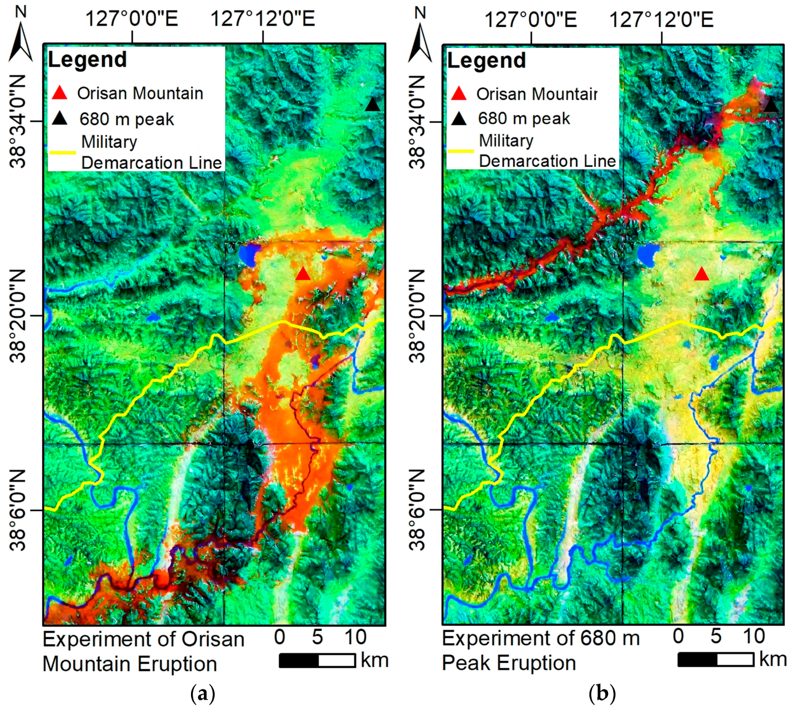
3.1. Experimental Results

The experimental results were divided into two processes: (1) the single eruptive vent from Orisan Mountain, as shown in Figure 6a, and (2) the single eruptive vents from the 680 m peak, as shown in Figure 6b. The experimental results were captured and processed using the georeferencing tool in GIS. The experimental results show that a 29 mL solution was used for the eruption of Orisan Mountain and 13 mL was used for the eruption from the 680 m peak. The volume of the lava in the actual eruption can be calculated by assuming that the parameters of the lava thickness and the effusion rate were similar to the Mauna Loa 1984 eruption of approximately 3 m and 100 m3/s, respectively [69]. Assuming the injected simulated lava has three-dimensionally equal sides, we can limit the vertical scale to 1:100, and thus the volume of injected simulated lava was equivalent to 6 . 75   ×   10 - 2 km3 in the Orisan Mountain eruption. The result from the experimental eruption from the 680 m peak was unsuccessful because the topographical map had a channel down in the southwest direction from the eruption source. Due to the unavailability of the paleotopographical map from the pre-eruption, the analysis for the eruption of the 680 m peak remained unsolved. Otherwise, the experimental result from Orisan Mountain was available for the eruption to flow down to the south through the Hantangang River and pass through the southwest across the Imjingang River. The experimental result analysis was conducted using the pixel-based classification method. The classification was conducted on only the four pieces of the 3D terrain model, while the two pieces that contained the 680 m peak and the left side that was not needed for classification were removed for the effectiveness of the classification process.

3.2. Classification Results

The experimental results from the four pieces of the 3D terrain model in Figure 7a were captured and georeferenced before the classification process. The experimental image was classified as the simulated lava area and the 3D terrain model, which did not include the simulated lava from the experiment. The classification process was initiated with a stratified random sampling method on a pixel-by-pixel basis. We sampled twenty random polygons for the simulated lava category with similar colors and twenty random polygons for the 3D terrain model of the area that did not consist of simulated lava with different colors. Twenty samples of each category were divided into a 70:30 ratio of the dataset for the training and testing process to have optimal results [80,81,82]. A total of 28 samples was used as the training sample for classification analysis using the ANN and SVM algorithms, and 12 samples were used as testing samples for the validation analysis [36,38].
The classification results from the ANN algorithm and SVM algorithm are shown in Figure 7b,c. The classification result from the SVM algorithm was shown to better recognize the lava flows, as the lava flows were connected from the lava eruption source to the southern area through the Hantangang River. Moreover, the classification result from the ANN algorithm left traces of the lava flow that were not connected to some part of the southern area of the images. The ANN classified these areas as non-simulated lava due to the similar color of the gap within the lava flow between each piece of the 3D terrain model. The geological landform in Figure 7d was used to accurately assess the experimental results with the ground truth data.

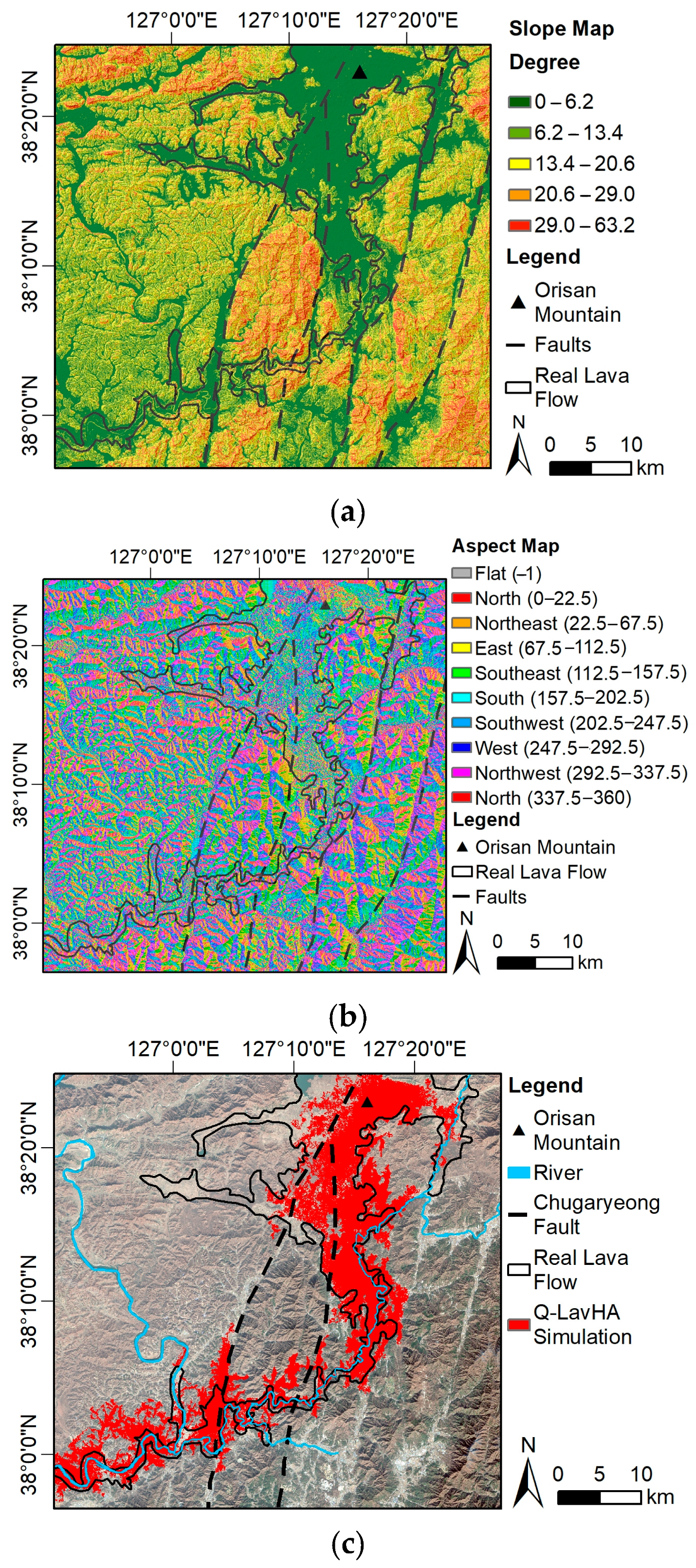
3.3. Q-LavHA Simulation Results

The Q-LavHA simulation process was similar to the experimental process in selecting the eruptive vent: (1) the single eruptive vent from Orisan Mountain, as shown in Figure 8a, and (2) the single eruptive vent from the 680 m peak, as shown in Figure 8b. The result from the eruption of the 680 m peak shows that the simulated lava did not flow down to the southern area, as it should have due to the existence of the channel river close to the location of the 680 m peak, and made the probability of the lava flows unable to flow across the river. The result was consistent with the experimental process in the 680 m peak eruption, and because of the condition of the topography, further analysis was not available. Moreover, the flow from the Orisan Mountain eruption stopped before reaching the Hantangang River. This condition suggests that the lava was losing its velocity before reaching the river because the topographic conditions in that area were a low elevation area with a gentle slope.
The evaluation criteria from the Q-LavHA simulation result are shown in Table 2. The overall accuracy of the Orisan Mountain eruption was 2.32% higher than that of the 680 m peak. The error rate shows that the Orisan Mountain eruption had a lower error rate of approximately 2.32% than the eruption of the 680 m peak. The very low true positive rate from the 680 m peak eruption (5.68%) indicates that the probability of the lava simulation at the 680 m peak eruption was only 5.68% predicted and observed in the ground truth data. We used a 5000 m3/s effusion rate as the highest effusion rate in recorded history [7] with 100 Pa-s initial viscosity as the lowest viscosity of the typical basaltic lava at 1200 °C at low pressure [73]. These parameters were used in the Q-LavHA simulation for both simulation processes. The Discussion section explains the further analysis of the simulation process to understand the relation between the effusion rate and the simulated lava dimension in the Q-LavHA simulation process.

4. Discussion

4.1. Experimental Accuracy

The model performance evaluation was assessed using quantitative analysis based on the producer’s accuracy, user’s accuracy, overall accuracy, and Kappa coefficient. The producer’s accuracy defines the omission errors and the accuracy from the point of view of the producer of the classified map describing the percentage of ground truth data is displayed on the classified map. The user’s accuracy defines the omission errors for each classification class from the point of view of the user’s map; the reliability of the classified map is described based on the ground truth data [83,84]. The overall accuracy describes the ratio of the accurately classified areas based on each class. The kappa coefficient determines the degree of match between the classification result and the reference data [85]. In this case, for validation, we used the testing data to assess the accuracy of the classification method based on the ANN and SVM algorithms. The confusion matrix assessed the quantitative analysis based on the value of true positives and true negatives as the correctly classified area and false positives and false negatives as the incorrectly classified area. The results of the accuracy assessment are shown in Table 3.
The producer’s accuracy of the simulated lava and the 3D terrain model was shown to be higher in the SVM algorithm, for which the values were approximately 0.49% and 0.01%, respectively, compared with the ANN algorithm. The higher user’s accuracy of the simulated lava and the 3D terrain model from the SVM algorithm means that the SVM algorithm was better at identifying the simulated lava by approximately 0.11% and 0.05% for the 3D terrain model compared with the ANN algorithm. The overall accuracy and kappa coefficient were consistent with the previous quantitative analysis that the classification result from the SVM algorithm was better than the ANN algorithm of approximately 0.06% for overall accuracy and 0.01% for the kappa coefficient.
The classification result was compared with the ground truth data by utilizing a confusion matrix algorithm that assessed the values of true positives, false positives, false negatives, and true negatives between the predicted cases using the experimental lava eruption from Orisan Mountain through a 3D terrain model. Binary classification between the pixels of the classification result and the ground truth data was evaluated with the advanced metric from Equations (8)–(13). The evaluation criteria between the ANN and SVM classification results are shown in Table 4. The overall accuracy of the SVM algorithm was higher, at 0.76%, than that of the ANN algorithm, and the SVM algorithm had a 0.76% lower error rate than the ANN algorithm. A higher rate of true positives and true negatives with a lower rate of false positives and false negatives was shown in the SVM algorithm result, which indicates that the classification result from the SVM algorithm was better than that from the ANN algorithm.
The higher accuracy of the SVM algorithm for classification was consistent with the classification study that implemented the SVM and ANN in their study [34,35,36,38]. The SVM algorithm was afforded a better recognition rate than the ANN algorithm because the SVM algorithm was able to find solutions in the training process by considering the structural risk in model complexity [86]. In addition to the higher accuracy, the SVM algorithm was computationally more efficient than the ANN algorithm. This process was consistent with the classification studies that utilized the SVM and ANN algorithms in their study [34,36]. The higher time consumption that the ANN algorithm used to classify the training sample was because the number of iterations in the training process affected the time required to recognize the pattern in the hidden layer [36]. Moreover, the SVM has the advantage of classifying the two classes within the margin width in the hyperplane in its simplest form [27].

4.2. Effusion Rate Analysis of Q-LavHA

Further analysis of the single eruptive vent on Orisan Mountain was conducted only in the southern area of the Hantangang River, as shown in Figure 9a, with a similar boundary to Figure 7a. The simulated lava with different effusion rates is shown in Figure 9b. We simulated the lava with the lowest effusion rate as the highest possible effusion rate in recorded history for the Laki eruption in Iceland [7]. The relation between the effusion rate (m3/s) and the lava dimension (km2) was extracted from the geometry calculation from the simulation result. We plotted the data as shown on the graph in Figure 9c. The Euclidean distance tool was used to construct the distance map to analyze the lava dimension. The simulated lava dimension is shown in Figure 9d and shows that the highest dimension was approximately 472 km2. Using the equation in Figure 9c, the effusion rate needed for simulation was approximately 70,608 m3/s. This effusion rate was too large to be simulated in Q-LavHA and transformed the simulation process into errors in the program. Another approach could be conducted by implementing multiple vent eruptions. Possible coordinates of eruptive vents were selected in the area with a higher elevation and downslope in the south and southwest directions, thereby forcing the lava to flow to the tip of the ground truth data.

4.3. Multiple Vent Eruption

An analysis of the topographical conditions in the study area should be conducted to assess the potential eruptive vent for the case of a multiple vent eruption. The slope map (Figure 10a) and aspect map (Figure 10b) were generated from the elevation map in Figure 9a to analyze the probable location of an eruptive vent that may produce a lava flow that is close to the geological landform of the Hantangang basalt in the study area. Kil et al. (2019) assumed that the volcanic sources were aligned with the Chugaryeong Fault and that fissure eruption occurred due to fractures caused by fault movement [14]. The lava flow simulation on the Hantangang River had a similar challenge as the historical case of Paricutin Volcano, which erupted from a gentle slope (the real lava flow slope area ranges from 0° to 6.2° in Figure 10a). Becerril et al. (2021) modified the location of the vent or fissure location to the most suitable downslope direction (aspect map in Figure 10b). In this study, the most suitable assumption of the probable vent was the area that had a high elevation and slope that aligned along the Chugaryeong Fault. The downslope direction of the probable vent or fissure was toward the southwest to obtain a good fit for the flow propagation to the tip of the real lava flow [42]. The slope and aspect maps identified the degree and downslope direction of the maximum rate of change from the DEM cell to its neighbors [42,87].
We selected the probable eruptive vent based on the study area′s slope and aspect maps, as shown in Table 5. The first eruptive vent was the Orisan Mountain location, with a southward downslope direction with a slope of approximately 1.06°, extending approximately 51.035 km2 from the eruption site. The second eruptive vent was chosen in the western Yangji-ri area, with an altitude of approximately 283 m and a slope of approximately 23.02° in the southwest direction. The third eruptive vent was located across the Chugaryeong fault, with an altitude of approximately 206 m and a slope of approximately 30.75° toward the southwest. The fourth eruptive vent was located around the Chugaryeong fault, with an elevation of approximately 62 m and a slope of approximately 22.68° that has a downslope in the southwest direction. These adjustments, in addition to the eruptive vent in the eruption, were needed to overcome the limitation of the availability of the paleotopographical map before the Orisan Mountain eruption.
The result from the multiple vent eruption is shown in Figure 10c and the accuracy of the simulated lava flow was assessed by comparing it with the real lava flow (Figure 7d). The accuracy assessment resulted in an overall accuracy of approximately 87.54%, with an error rate of approximately 12.46%. These values were approximately 2.5% higher for the overall accuracy, and approximately 2.5% lower for the error rate compared with the experimental result accuracy. The true positive rate, false negative rate, false positive, and true negative rate represented the well-simulated area, underestimated, overestimated, and non-estimated area. The well-simulated or overlapping area between the simulated lava flow and the real lava flow was 58.58%. The underestimation or the condition of the real lava flow area that did not appear in the simulated lava flow was approximately 41.54%. The overestimated area or the mismatch of the simulated lava flow that exceeded the real lava flow area was approximately 6.83%. The area that was not supposed to be estimated in the real lava flow by the simulation was shown at approximately 93.17%.

5. Conclusions

The experiment and simulation of the Hantangang River Volcanic Field were conducted to study the prehistorical eruption of Orisan Mountain that formed the present-day Hantangang River Volcanic Field (HRVF). The experiment and simulation were conducted by utilizing the DEM SRTM for generating the 3D-printed terrain model and the input of the simulation process, respectively. The results from both methods were compared by their accuracies and showed that the result from the advanced metric of the confusion matrix from the experimental processing was 25.98% higher (accuracy of the SVM classification compared with the ground truth data) than the Q-LavHA simulation in the case of a single eruptive vent from Orisan Mountain. The results from both the experiment and simulation for the case of the single eruptive vent from the 680 m peak eruption could not be further analyzed due to the existence of the river near the location of the 680 m peak. Most of the simulated lava from the experiment and Q-LavHA flowed toward the river outside the real lava flow boundary. The Q-LavHA simulation′s limitation was that the topographical conditions of the available digital elevation model did not represent the topographical conditions of the Hantangang River Volcanic Field (HRVF) before the eruption.
The limitation of the unavailability of the paleotopography of the Hantangang River Volcanic Field was overcome by the additional eruptive vent in the study area. The additional eruptive vent was analyzed using slope and aspect maps in the study area. A slope higher than 20° with the downslope direction toward the tip of the real lava flow directed toward the southwest was chosen as a probable vent for the simulation process. The results show higher accuracy in the well-simulated area than the real lava flow. The well-simulated area was 41.76% and 15.78% higher in the multiple vent eruption than in the single eruptive vent from the Q-LavHA simulation and the experiment from the 3D terrain model, respectively. This research could become a preliminary study related to the origin of the Hantangang River Volcanic Field. For better interpretation, further research could be conducted by generating paleotopography for the Hantangang River and Orisan Mountain before the eruption.

Author Contributions

Conceptualization: C.-W.L., S.P., B.K. and W.L.H.; methodology: C.-W.L., S.P. and W.L.H.; software: S.R. and W.L.H.; validation: C.-W.L. and W.L.H.; formal analysis: W.L.H.; investigation: C.-W.L., S.P. and S.R.; resources: C.-W.L., D.-K.C., B.K. and S.P.; data curation: C.-W.L., B.K. and W.L.H.; writing—original draft preparation: W.L.H.; writing—review and editing: C.-W.L., B.K., S.R. and W.L.H.; visualization: C.-W.L., S.R., D.-K.C. and W.L.H.; supervision: C.-W.L., B.K. and S.P.; project administration: C.-W.L.; funding acquisition: C.-W.L. and D.-K.C. All authors have read and agreed to the published version of the manuscript.

Funding

This research was supported by the 2021 Research Project for the UNESCO Hantangang River Global Geopark and the Gyeonggi Provincial Office.

Institutional Review Board Statement

Not applicable.

Informed Consent Statement

Not applicable.

Data Availability Statement

The DEM SRTM data used in this study were obtained from the United States Geological Survey (USGS) (https://earthexplorer.usgs.gov/ (accessed on 21 October 2021).

Conflicts of Interest

The authors declare no conflict of interest. The funders had no role in the design of the study; in the collection, analysis, or interpretation of the data; in the writing of the manuscript; or in the decision to publish the results.

References

  1. Self, S. The effects and consequences of very large explosive volcanic eruptions. Philos. Trans. R. Soc. A Math. Phys. Eng. Sci. 2006, 364, 2073–2097. [Google Scholar] [CrossRef] [PubMed]
  2. Newhall, C.G.; Self, S. The volcanic explosivity index (VEI): An estimate of explosive magnitude for historical volcanism. J. Geophys. Res. 1982, 87, 1231–1238. [Google Scholar] [CrossRef]
  3. Pyle, D.M. Sizes of Volcanic Eruptions, 2nd ed.; Elsevier Inc.: Amsterdam, The Netherlands, 2015; ISBN 9780123859389. [Google Scholar]
  4. Mason, B.G.; Pyle, D.M.; Oppenheimer, C. The size and frequency of the largest explosive eruptions on Earth. Bull. Volcanol. 2004, 66, 735–748. [Google Scholar] [CrossRef]
  5. Scandone, R.; Bartolini, S.; Martí, J. A scale for ranking volcanoes by risk. Bull. Volcanol. 2016, 78, 2. [Google Scholar] [CrossRef]
  6. Harris, A.J.L.; Dehn, J.; Calvari, S. Lava effusion rate definition and measurement: A review. Bull. Volcanol. 2007, 70, 1. [Google Scholar] [CrossRef]
  7. Thordarson, T.; Self, S. Atmospheric and environmental effects of the 1783-1784 Laki eruption: A review and reassessment. J. Geophys. Res. Atmos. 2003, 108, AAC-7. [Google Scholar] [CrossRef] [Green Version]
  8. Keszthelyi, L.; Self, S. Some physical requirements for the emplacement of long basaltic lava flows. J. Geophys. Res. Solid Earth 1998, 103, 27447–27464. [Google Scholar] [CrossRef] [Green Version]
  9. Miyamoto, H.; Sasaki, S. Numerical simulations of flood basalt lava flows: Roles of parameters on lava flow morphologies. J. Geophys. Res. Solid Earth 1998, 103, 27489–27502. [Google Scholar] [CrossRef] [Green Version]
  10. Weon, J.K. A study on the Quaternary volcanism in the Korean Peninsula–in the Choogaryong Rift Valley. J. Geol. Soc. Korea 1983, 19, 159–168. [Google Scholar]
  11. Won, C.K.; Kim, Y.K.; Lee, M.W. The study on the geochemistry of Choogaryong alkali basalt. J. Geol. Soc. Korea 1990, 26, 70–81. [Google Scholar]
  12. Lee, D.S.; Ryu, K.J.; Kim, K.H. Geotectonic interpretation of Choogaryong Rift Valley, Korea. J. Geol. Soc. Korea 1983, 19, 19–38. [Google Scholar]
  13. Ryu, S.; Oka, M.; Yagi, K.; Sakuyama, T.; Itaya, T. K-Ar ages of the Quaternary basalts in the Jeongok area, the central part of Korean Peninsula. Geosci. J. 2011, 15, 1–8. [Google Scholar] [CrossRef]
  14. Kil, Y.; Ahn, K.S.; Woo, K.S.; Lee, K.C.; Jwa, Y.-J.; Jung, W.; Sohn, Y.K. Geoheritage Values of the Quaternary Hantangang River Volcanic Field in the Central Korean Peninsula. Geoheritage 2019, 11, 765–782. [Google Scholar] [CrossRef]
  15. Woo, K.S.; Sohn, Y.K.; Kil, Y.; Jwa, Y.J.; Ju, S.O. The aspiring Hantangang Global Geopark in Korea: Justification to be endorsed by UNESCO Global Geopark. In Proceedings of the EGU General Assembly, Vienna, Austria, 8–13 April 2018; Volume 20, p. 2935. [Google Scholar]
  16. Hasiuk, F. Making things geological: 3-D printing in the geosciences. GSA Today 2014, 24, 28–29. [Google Scholar] [CrossRef] [Green Version]
  17. Bishwal, R.M. Scope of 3-D Printing in Mining and Geology: An Overview. J. Geol. Soc. India 2019, 93, 482–486. [Google Scholar] [CrossRef]
  18. Kyriakopoulos, C. 3D printing: A remedy to common misconceptions about earthquakes. Seismol. Res. Lett. 2019, 90, 1689–1691. [Google Scholar] [CrossRef]
  19. Zhang, G.; Gong, J.; Li, Y.; Sun, J.; Xu, B.; Zhang, D.; Zhou, J.; Guo, L.; Shen, S.; Yin, B. An efficient flood dynamic visualization approach based on 3D printing and augmented reality. Int. J. Digit. Earth 2020, 13, 1302–1320. [Google Scholar] [CrossRef]
  20. Liang, T.; Knappett, J.A.; Bengough, A.G.; Ke, Y.X. Small-scale modelling of plant root systems using 3D printing, with applications to investigate the role of vegetation on earthquake-induced landslides. Landslides 2017, 14, 1747–1765. [Google Scholar] [CrossRef] [Green Version]
  21. Horowitz, S.S.; Schultz, P.H. Printing space: Using 3D printing of digital terrain models in geosciences education and research. J. Geosci. Educ. 2014, 62, 138–145. [Google Scholar] [CrossRef]
  22. Wabiński, J.; Mościcka, A. Natural heritage reconstruction using full-color 3D Printing: A case study of the valley of five Polish ponds. Sustainability 2019, 11, 5907. [Google Scholar] [CrossRef] [Green Version]
  23. Kumari, R.; Kr, S. Machine Learning: A Review on Binary Classification. Int. J. Comput. Appl. 2017, 160, 11–15. [Google Scholar] [CrossRef]
  24. Kotsiantis, S.B. Supervised Machine Learning: A Review of Classification Techniques. Informatica 2007, 31, 249–269. [Google Scholar]
  25. Maxwell, A.E.; Warner, T.A.; Fang, F. Implementation of machine-learning classification in remote sensing: An applied review. Int. J. Remote Sens. 2018, 39, 2784–2817. [Google Scholar] [CrossRef] [Green Version]
  26. Sheykhmousa, M.; Mahdianpari, M.; Ghanbari, H.; Mohammadimanesh, F.; Ghamisi, P.; Homayouni, S. Support Vector Machine Versus Random Forest for Remote Sensing Image Classification: A Meta-Analysis and Systematic Review. IEEE J. Sel. Top. Appl. Earth Obs. Remote Sens. 2020, 13, 6308–6325. [Google Scholar] [CrossRef]
  27. Mountrakis, G.; Im, J.; Ogole, C. Support vector machines in remote sensing: A review. ISPRS J. Photogramm. Remote Sens. 2011, 66, 247–259. [Google Scholar] [CrossRef]
  28. Mohanty, K.K.; Majumdar, T.J. An artificial neural network (ANN) based software package for classification of remotely sensed data. Comput. Geosci. 1996, 22, 81–87. [Google Scholar] [CrossRef]
  29. Jeatrakul, P.; Wong, K.W. Comparing the performance of different neural networks for binary classification problems. In Proceedings of the 2009 Eighth International Symposium on Natural Language Processing, Bangkok, Thailand, 20–22 October 2009; pp. 111–115. [Google Scholar] [CrossRef] [Green Version]
  30. Faris, H.; Aljarah, I.; Mirjalili, S. Training feedforward neural networks using multi-verse optimizer for binary classification problems. Appl. Intell. 2016, 45, 322–332. [Google Scholar] [CrossRef]
  31. Roßbach, P. Neural Networks vs. Random Forests—Does it always have to be Deep Learning. Ger. Frankf. Sch. Financ. Manag. 2018. Available online: https://blog.frankfurt-school.de/wp-content/uploads/2018/10/Neural-Networks-vs-Random-Forests.pdf (accessed on 1 February 2022).
  32. Ahmad, M.W.; Mourshed, M.; Rezgui, Y. Trees vs Neurons: Comparison between random forest and ANN for high-resolution prediction of building energy consumption. Energy Build. 2017, 147, 77–89. [Google Scholar] [CrossRef]
  33. Boateng, E.Y.; Otoo, J.; Abaye, D.A. Basic Tenets of Classification Algorithms K-Nearest-Neighbor, Support Vector Machine, Random Forest and Neural Network: A Review. J. Data Anal. Inf. Process. 2020, 08, 341–357. [Google Scholar] [CrossRef]
  34. Kadavi, P.R.; Lee, C.-W. Land cover classification analysis of volcanic island in Aleutian Arc using an artificial neural network (ANN) and a support vector machine (SVM) from Landsat imagery. Geosci. J. 2018, 22, 653–665. [Google Scholar] [CrossRef]
  35. Syifa, M.; Park, S.J.; Lee, C.W. Detection of the Pine Wilt Disease Tree Candidates for Drone Remote Sensing Using Artificial Intelligence Techniques. Engineering 2020, 6, 919–926. [Google Scholar] [CrossRef]
  36. Nur, A.S.; Park, S.; Lee, K.J.; Moon, J.; Lee, C.W. Mapping of post-wildfire burned area using KOMPSAT-3A and sentinel-2 imagery: The case of Sokcho wildfire, Korea. Korean J. Remote Sens. 2020, 36, 1551–1565. [Google Scholar] [CrossRef]
  37. Syifa, M.; Kadavi, P.R.; Lee, C.W.; Pradhan, B. Landsat images and artificial intelligence techniques used to map volcanic ashfall and pyroclastic material following the eruption of Mount Agung, Indonesia. Arab. J. Geosci. 2020, 13, 133. [Google Scholar] [CrossRef]
  38. Syifa, M.; Kadavi, P.; Lee, C.-W. An Artificial Intelligence Application for Post-Earthquake Damage Mapping in Palu, Central Sulawesi, Indonesia. Sensors 2019, 19, 542. [Google Scholar] [CrossRef] [PubMed] [Green Version]
  39. Kadavi, P.R.; Lee, W.J.; Lee, C.W. Analysis of the pyroclastic flow deposits of Mount Sinabung and Merapi using Landsat imagery and the artificial neural networks approach. Appl. Sci. 2017, 7, 935. [Google Scholar] [CrossRef] [Green Version]
  40. Syifa, M.; Panahi, M.; Lee, C.W. Mapping of post-wildfire burned area using a hybrid algorithm and satellite data: The case of the camp fire wildfire in California, USA. Remote Sens. 2020, 12, 623. [Google Scholar] [CrossRef] [Green Version]
  41. Mossoux, S.; Saey, M.; Bartolini, S.; Poppe, S.; Canters, F.; Kervyn, M. Q-LAVHA: A flexible GIS plugin to simulate lava flows. Comput. Geosci. 2016, 97, 98–109. [Google Scholar] [CrossRef]
  42. Becerril, L.; Larrea, P.; Salinas, S.; Mossoux, S.; Ferrés, D.; Widom, E.; Siebe, C.; Martí, J. The historical case of Paricutin volcano (Michoacán, México): Challenges of simulating lava flows on a gentle slope during a long-lasting eruption. Nat. Hazards 2021, 107, 809–829. [Google Scholar] [CrossRef]
  43. Prieto-Torrell, C.; Rodriguez-Gonzalez, A.; Aulinas, M.; Fernandez-Turiel, J.L.; Cabrera, M.C.; Criado, C.; Perez-Torrado, F.J. Modelling and simulation of a lava flow affecting a shore platform: A case study of Montaña de Aguarijo eruption, El Hierro (Canary Islands, Spain). J. Maps 2021, 17, 502–511. [Google Scholar] [CrossRef]
  44. Dille, A.; Poppe, S.; Mossoux, S.; Soulé, H.; Kervyn, M. Modeling Lahars on a Poorly Eroded Basaltic Shield: Karthala Volcano, Grande Comore Island. Front. Earth Sci. 2020, 8, 1–17. [Google Scholar] [CrossRef]
  45. Oswald, C.; Rinner, C.; Robinson, A. Applications of 3D printing in physical geography education and urban visualization. Cartographica 2019, 54, 278–287. [Google Scholar] [CrossRef]
  46. Rodriguez-Gonzalez, A.; Aulinas, M.; Mossoux, S.; Perez-Torrado, F.J.; Fernandez-Turiel, J.L.; Cabrera, M.; Prieto-Torrell, C. Comparison of real and simulated lava flows in the Holocene volcanism of Gran Canaria (Canary Islands, Spain) with Q-LavHA: Contribution to volcanic hazard management. Nat. Hazards 2021, 107, 1785–1819. [Google Scholar] [CrossRef]
  47. Lee, Y.S.; Min, K.D.; Hwang, J.H. The Geodynamic Evolution of the Chugaryeong Fault Valley in a View Point of Paleomagnetism. Econ. Environ. Geol. 2001, 34, 555–571. [Google Scholar]
  48. Kee, W.S.; Lim, S.B.; Kim, H.C.; Kim, B.C.; Hwang, S.K.; Song, K.Y.; Kim, Y.H. Geological Report of the Yeoncheon Sheet (1:50,000); Korea Institute of Geoscience and Mineral Resources (KIGAM): Daejeon, Korea, 2008. [Google Scholar]
  49. Shin, S.; Cheon, Y.; Choi, J.H.; Cheong, D.; Choi, S.Y.; Lim, H.S.; Bae, H.; Lee, H.K. Late Pleistocene sedimentary environment and reverse faulting along the Chugaryung Fault in the central Korean Peninsula: A case study on the Cheorwon Basin. Geosci. J. 2020, 24, 615–623. [Google Scholar] [CrossRef]
  50. Choi, S.-J.; Chwae, U.-C.; Lee, H.-K.; Song, Y.-G.; Kang, I.-M. Review on the Chugaryeong Fault. Econ. Environ. Geol. 2012, 45, 441–446. [Google Scholar] [CrossRef] [Green Version]
  51. Nagaoka, S.; Danhara, T.; Itaya, T.; Sakuyama, T.; Watanabe, M.; Bae, K.; Matsufuji, K. Stratigraphy and age of Quaternary basaltic lavas and reconstruction of paleogeography in Chongokni, Korea. In Loess-Paleosol and Paleolithic Chronology in East Asia; Matsufuji, K., Ed.; Yuzankaku: Tokyo, Japan, 2008; pp. 87–102. [Google Scholar]
  52. Farr, T.G.; Rosen, P.A.; Caro, E.; Crippen, R.; Duren, R.; Hensley, S.; Kobrick, M.; Paller, M.; Rodriguez, E.; Roth, L.; et al. The Shuttle Radar Topography Mission. Rev. Geophys. 2007, 45, RG2004. [Google Scholar] [CrossRef] [Green Version]
  53. Purinton, B.; Bookhagen, B. Validation of digital elevation models (DEMs) and comparison of geomorphic metrics on the southern Central Andean Plateau. Earth Surf. Dyn. 2017, 5, 211–237. [Google Scholar] [CrossRef] [Green Version]
  54. Van Zyl, J.J. The shuttle radar topography mission (SRTM): A breakthrough in remote sensing of topography. Acta Astronaut. 2001, 48, 559–565. [Google Scholar] [CrossRef]
  55. Rabus, B.; Eineder, M.; Roth, A.; Bamler, R. The shuttle radar topography mission—A new class of digital elevation models acquired by spaceborne radar. ISPRS J. Photogramm. Remote Sens. 2003, 57, 241–262. [Google Scholar] [CrossRef]
  56. Smith, B.; Sandwell, D. Accuracy and resolution of shuttle radar topography mission data. Geophys. Res. Lett. 2003, 30, 3–6. [Google Scholar] [CrossRef] [Green Version]
  57. Alganci, U.; Besol, B.; Sertel, E. Accuracy assessment of different digital surface models. ISPRS Int. J. Geo-Inf. 2018, 7, 114. [Google Scholar] [CrossRef] [Green Version]
  58. Stoter, J.; Post, M.; Van Altena, V.; Nijhuis, R.; Bruns, B. Fully automated generalization of a 1:50k map from 1:10k data. Cartogr. Geogr. Inf. Sci. 2014, 41, 1–13. [Google Scholar] [CrossRef]
  59. Hasiuk, F.; Harding, C. Touchable topography: 3D printing elevation data and structural models to overcome the issue of scale. Geol. Today 2016, 32, 16–20. [Google Scholar] [CrossRef]
  60. Hasiuk, F.J.; Harding, C.; Renner, A.R.; Winer, E. TouchTerrain: A simple web-tool for creating 3D-printable topographic models. Comput. Geosci. 2017, 109, 25–31. [Google Scholar] [CrossRef]
  61. Han, S.-H.; Kim, K.W.; Kim, S.; Youn, Y.C. Artificial Neural Network: Understanding the Basic Concepts without Mathematics. Dement. Neurocognitive Disord. 2018, 17, 83. [Google Scholar] [CrossRef] [PubMed]
  62. Pham, B.T.; Tien Bui, D.; Prakash, I.; Dholakia, M.B. Hybrid integration of Multilayer Perceptron Neural Networks and machine learning ensembles for landslide susceptibility assessment at Himalayan area (India) using GIS. Catena 2017, 149, 52–63. [Google Scholar] [CrossRef]
  63. Gardner, M.W.; Dorling, S.R. Artificial neural networks (the multilayer perceptron)—A review of applications in the atmospheric sciences. Atmos. Environ. 1998, 32, 2627–2636. [Google Scholar] [CrossRef]
  64. Cortes, C.; Vapnik, V. Support-vector networks. Mach. Learn. 1995, 20, 273–297. [Google Scholar] [CrossRef]
  65. Prasad, P.; Loveson, V.J.; Kotha, M.; Yadav, R. Application of machine learning techniques in groundwater potential mapping along the west coast of India. GIScience Remote Sens. 2020, 57, 735–752. [Google Scholar] [CrossRef]
  66. Liu, Y.; Zhang, B.; Wang, L.; Wang, N. A self-trained semisupervised SVM approach to the remote sensing land cover classification. Comput. Geosci. 2013, 59, 98–107. [Google Scholar] [CrossRef]
  67. Soman, K.; Sathiya, A.; Suganthi, N. Classification of stress of automobile drivers using Radial Basis Function Kernel Support Vector Machine. In Proceedings of the International Conference on Information Communication and Embedded Systems (ICICES2014), Chennai, India, 27–28 February 2015. [Google Scholar] [CrossRef]
  68. Felpeto, A.; Araña, V.; Ortiz, R.; Astiz, M.; García, A. Assessment and modelling of lava flow hazard on Lanzarote (Canary Islands). Nat. Hazards 2001, 23, 247–257. [Google Scholar] [CrossRef]
  69. Harris, A.J.L.; Rowland, S.K. FLOWGO: A kinematic thermo-rheological model for lava flowing in a channel. Bull. Volcanol. 2001, 63, 20–44. [Google Scholar] [CrossRef]
  70. Favalli, M.; Mazzarini, F.; Pareschi, M.T.; Boschi, E. Topographie control on lava flow paths at Mount Etna, Italy: Implications for hazard assessment. J. Geophys. Res. Earth Surf. 2009, 114, 1–13. [Google Scholar] [CrossRef]
  71. Kereszturi, G.; Cappello, A.; Ganci, G.; Procter, J.; Németh, K.; Del Negro, C.; Cronin, S.J. Numerical simulation of basaltic lava flows in the auckland volcanic field, New Zealand—implication for volcanic hazard assessment. Bull. Volcanol. 2014, 76, 879. [Google Scholar] [CrossRef]
  72. Dragoni, M. A dynamical model of lava flows cooling by radiation. Bull. Volcanol. 1989, 51, 88–95. [Google Scholar] [CrossRef]
  73. Lesher, C.E.; Spera, F.J. Thermodynamic and Transport Properties of Silicate Melts and Magma, 2nd ed.; Elsevier Inc.: Amsterdam, The Netherlands, 2015; ISBN 9780123859389. [Google Scholar]
  74. Pontius, R.G.; Millones, M. Death to Kappa: Birth of quantity disagreement and allocation disagreement for accuracy assessment. Int. J. Remote Sens. 2011, 32, 4407–4429. [Google Scholar] [CrossRef]
  75. Saito, T.; Rehmsmeier, M. The precision-recall plot is more informative than the ROC plot when evaluating binary classifiers on imbalanced datasets. PLoS ONE 2015, 10, e0118432. [Google Scholar] [CrossRef] [Green Version]
  76. Beauxis-aussalet, E.; Hardman, L. Visualization of Confusion Matrix for Non-Expert Users. In IEEE Conference on Visual Analytics Science and Technology (VAST)-Poster Proceedings; 2014; Available online: https://ir.cwi.nl/ (accessed on 22 December 2021).
  77. Ohsaki, M.; Wang, P.; Matsuda, K.; Katagiri, S.; Watanabe, H.; Ralescu, A. Confusion-matrix-based kernel logistic regression for imbalanced data classification. IEEE Trans. Knowl. Data Eng. 2017, 29, 1806–1819. [Google Scholar] [CrossRef]
  78. Rahmati, O.; Moghaddam, D.D.; Moosavi, V.; Kalantari, Z.; Samadi, M.; Lee, S.; Bui, D.T. An automated Python language-based tool for creating absence samples in groundwater potential mapping. Remote Sens. 2019, 11, 1375. [Google Scholar] [CrossRef] [Green Version]
  79. Pham, B.T.; Shirzadi, A.; Shahabi, H.; Omidvar, E.; Singh, S.K.; Sahana, M.; Asl, D.T.; Bin Ahmad, B.; Quoc, N.K.; Lee, S. Landslide susceptibility assessment by novel hybrid machine learning algorithms. Sustainability 2019, 11, 4386. [Google Scholar] [CrossRef] [Green Version]
  80. Hakim, W.L.; Rezaie, F.; Nur, A.S.; Panahi, M.; Khosravi, K.; Lee, C.-W.; Lee, S. Convolutional neural network (CNN) with metaheuristic optimization algorithms for landslide susceptibility mapping in Icheon, South Korea. J. Environ. Manag. 2022, 305, 114367. [Google Scholar] [CrossRef] [PubMed]
  81. Fadhillah, M.F.; Lee, S.; Lee, C.; Park, Y.-C. Application of Support Vector Regression and Metaheuristic Optimization Algorithms for Groundwater Potential Mapping in Gangneung-si, South Korea. Remote Sens. 2021, 13, 1196. [Google Scholar] [CrossRef]
  82. Hakim, W.L.; Nur, A.S.; Rezaie, F.; Panahi, M.; Lee, C.-W.; Lee, S. Convolutional neural network and long short-term memory algorithms for groundwater potential mapping in Anseong, South Korea. J. Hydrol. Reg. Stud. 2022, 39, 100990. [Google Scholar] [CrossRef]
  83. Congalton, R.G. A review of assessing the accuracy of classifications of remotely sensed data. Remote Sens. Environ. 1991, 37, 35–46. [Google Scholar] [CrossRef]
  84. Lyons, M.B.; Keith, D.A.; Phinn, S.R.; Mason, T.J.; Elith, J. A comparison of resampling methods for remote sensing classification and accuracy assessment. Remote Sens. Environ. 2018, 208, 145–153. [Google Scholar] [CrossRef]
  85. Mahdianpari, M.; Salehi, B.; Mohammadimanesh, F.; Motagh, M. Random forest wetland classification using ALOS-2 L-band, RADARSAT-2 C-band, and TerraSAR-X imagery. ISPRS J. Photogramm. Remote Sens. 2017, 130, 13–31. [Google Scholar] [CrossRef]
  86. Ren, J. ANN vs. SVM: Which one performs better in classification of MCCs in mammogram imaging. Knowl.-Based Syst. 2012, 26, 144–153. [Google Scholar] [CrossRef] [Green Version]
  87. Chang, K.T.; Tsai, B.W. The effect of dem resolution on slope and aspect mapping. Cartogr. Geogr. Inf. Syst. 1991, 18, 69–77. [Google Scholar] [CrossRef]
Figure 1. Location of the Hantangang River Volcanic Field (HRVF) from (a) the Korean Peninsula, with the segmented HRVF area modified from [14]; (b) digital terrain model of the study area depicted from the RGB composite of Sentinel-2 satellite imagery taken on 28 November 2021.
Remotesensing 14 00894 g001
Figure 2. Digital view of (a) the 3D terrain surface from DEM SRTM; (b) final model divided into 6 parts to fit the printer’s build size.
Remotesensing 14 00894 g002
Figure 3. (a) Materials for experimental processing; (b) top view of the 3D-printed model of the Hantangang River Volcanic Field and (c) bottom view of the 3D-printed model consisting of a transparent tube as the connector to the eruptive vent.
Remotesensing 14 00894 g003
Figure 4. Experimental procedure: (a) level check of the 3D terrain model; (b) initial conditions of the syringe filled with 50 mL of mixed ethanol; (c) composition of the experimental shoot for video recording.
Remotesensing 14 00894 g004
Figure 5. (a) Confusion matrix for binary classification; (b) schematic representation of the confusion matrix calculation.
Remotesensing 14 00894 g005
Figure 6. Experimental results of the lava flow simulation using the 3D-printed model from the (a) Orisan Mountain eruption and (b) 680 m peak eruption. The yellow line represents the boundary between South Korea and North Korea.
Remotesensing 14 00894 g006
Figure 7. (a) Experimental results of the lava flow simulation using the 3D-printed model from the (b) ANN classification result and (c) SVM classification result. (d) Real lava flows from the geological landform of the Hantangang River basalt from the Hantangang River volcanic field.
Remotesensing 14 00894 g007
Figure 8. Experimental results: (a) Orisan Mountain eruption; (b) 680 m peak eruption. The simulated lava flow is displayed with Sentinel-2 satellite imagery acquired from 20 September 2017.
Remotesensing 14 00894 g008
Figure 9. (a) Topographical map of the southern area of the Hantangang River Volcanic Field shown as an elevation map; (b) simulated lava flows with different effusion rates from Orisan Mountain; (c) relation between lava flow dimension and the lava effusion rate; (d) simulated lava dimensional flows.
Remotesensing 14 00894 g009
Figure 10. (a) Slope map; (b) aspect map; (c) Q-LavHA simulation of the multiple vent eruption case.
Remotesensing 14 00894 g010
Table 1. Parameters used for the Q-LavHA simulation using the L flowgo method.
Input ParametersSymbolUnitValuesSources
Velocity ConstantGravityg m / s 2 9.81Constant for Earth
Viscosity and Yield Strengthaa 1 / K 0.04[72]
bb Pa   s 0.01[72]
cc 1 / K 0.08[72]
Thermal ParametersEruption temperature T erupt °C1200[73]
Crust temperature T crust °C600[46]
Offset T crust T core °C150[46]
Thermal conductivity constantd-−0.16[41]
Crystal ParametersRate of crystallization δ ϕ micro δ T -0.004[46]
Latent heat of crystallization L cryst J / kg 5   ×   10 5 [73]
Inverse of maximum crystal concentrationR-1.51[69]
Conductivity ParametersLava thermal conductivity α lava W / mK 0.6[73]
Temperature at the base of the basalt crust T base °C700[69]
Thickness of the basalt crust H b %19[69]
Convection ParametersWind speedU m / s 5[69]
Friction   wind   speed Wind   speed 2   C h -0.0036[69]
Air temperature T air °C25[69]
Air density ρ air kg / m 3 0.4412Constant for Earth
Air specific heat capacity cp air J / kgK 1009Constant for Earth
Radiation ParametersStephan–Boltzmann constant σ J / m 2 K 4 5 . 67   ×   10 8 Constant for Earth
Emissivity of basalt ε -0.95Constant for Earth
Table 2. Comparison of evaluation criteria between the Orisan Mountain and 680 m peak eruptions compared with the ground truth data (of the HRVF).
Evaluation CriteriaOrisan Mountain680 m Peak
Overall Accuracy84.43%82.11%
Error Rate15.57%17.89%
True Positive Rate16.82%5.68%
False Positive Rate0.16%0.47%
False Negative Rate83.18%94.32%
True Negative Rate99.84%99.53%
Table 3. Accuracies of the simulated lava classification based on the ANN and SVM algorithms.
Classification ClassANNSVM
Producer’s
Accuracy (%)
User’s
Accuracy (%)
Overall
Accuracy
Kappa
Coefficient
Producer’s
Accuracy (%)
User’s
Accuracy (%)
Overall
Accuracy (%)
Kappa
Coefficient
Simulated Lava96.3699.7899.630.9796.8599.8999.690.98
3D Terrain Model99.9899.6299.9999.67
Table 4. Comparison of evaluation criteria between the classification result of the ANN and SVM compared with the ground truth data (of the HRVF).
Evaluation CriteriaANNSVM
Overall Accuracy84.28%85.04%
Error Rate15.72%14.96%
True Positive Rate17.55%42.80%
False Positive Rate11.93%6.79%
False Negative Rate82.45%57.20%
True Negative Rate88.07%93.21%
Table 5. Probable eruptive vent proposed to simulate the multiple vent eruption.
Eruptive Vent CoordinatesSlope (Degree)Aspect
127.267215°, 38.390937°1.06°206.29 (South)
127.262726°, 38.264870°23.02°208.07 (Southwest)
127.182083°, 38.069179°30.75°232.97 (Southwest)
127.088953°, 38.061274°22.68°203.50 (Southwest)
Publisher’s Note: MDPI stays neutral with regard to jurisdictional claims in published maps and institutional affiliations.

