3.2. Calibration and Validation Results
Table 3 gives a summary of the statistics for calibration and validation. Simulated and observed streamflow matched well in the calibration process for monthly and daily streamflow with E
NS = 0.86 and 0.85, respectively, as well as in the validation process with E
NS = 0.86 and 0.64 for monthly and daily streamflow, respectively (
Table 3). R
2 for monthly streamflow simulation in calibration and validation was 0.89 and 0.95, respectively, indicating a good linear relationship between simulated and observed data. Comparatively, R
2 for daily streamflow simulation in calibration and validation was relatively lower, namely, 0.65 and 0.64, respectively. The standard deviations (SDs) of observed values were bigger than those of simulated values, indicating actual streamflow variation was higher.
Table 3.
Evaluation of monthly and daily streamflow simulation.
Table 3.
Evaluation of monthly and daily streamflow simulation.
| | Monthly Streamflow (m3/s) | Daily Streamflow (m3/s) |
|---|
| Calibration | Validation | Calibration | Validation |
|---|
| Observed | Simulated | Observed | Simulated | Observed | Simulated | Observed | Simulated |
|---|
| Mean | 255.7 | 222.9 | 255.7 | 222.9 | 256.4 | 223.3 | 266.9 | 272.1 |
| SD
* | 194.9 | 176.3 | 246.0 | 227.5 | 314.3 | 254.4 | 314.3 | 254.4 |
| Sample numbers | 48 | 48 | 48 | 48 | 1,461 | 1,461 | 1,461 | 1,461 |
| ENS | 0.86 | 0.86 | 0.64 | 0.60 |
| R2 | 0.89 | 0.95 | 0.65 | 0.64 |
Prediction of monthly NH
4+-N and TP loads were both acceptable in the calibration process, with E
NS values of 0.69 and 0.56, respectively. In the validation process, the simulated and observed values of monthly NH
4+-N and TP also fitted marginally with E
NS = 0.57 and 0.49 (
Table 4). Meanwhile, R
2 for NH
4+-N and TP simulation in the calibration process was 0.71 and 0.90, respectively. R
2 for NH
4+-N and TP in the simulation in validation processes was 0.61 and 0.63, respectively.
Table 4.
Evaluation of monthly NH4+-N and TP simulation.
Table 4.
Evaluation of monthly NH4+-N and TP simulation.
| | Monthly NH4+-N Load | Monthly TP Load |
|---|
| Calibration | Validation | Calibration | Validation |
|---|
| ENS | 0.69 | 0.57 | 0.56 | 0.49 |
| R2 | 0.71 | 0.61 | 0.90 | 0.63 |
The results demonstrated that the SWAT, when calibrated, could provide good estimates of monthly and daily streamflow and monthly NH4+-N and TP loads. Overall, the SWAT performed better in simulating monthly and daily streamflow than monthly NH4+-N and TP loads.
3.3. Influence of LULC Datasets with Different Points in Time on Watershed Modeling
There were no significant differences in predicted monthly streamflow and daily streamflow when using LULC datasets with three points in time, namely, 2002 (02LU), 2007 (07LU) and 2010 (10LU) (
Table 5), indicating that the sensitivity of SWAT modeling of LULC datasets with different points in time was low in terms of streamflow simulation.
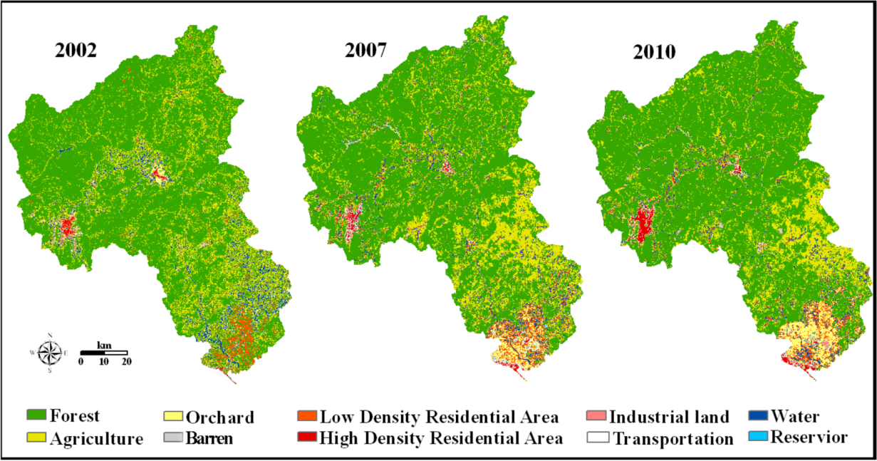
This phenomenon might be attributed to the fact that the study area had not undergone significant land use change over the period 2002–2010 and was also likely due to the comprehensive influence of land use and land cover changes. In this study, Forest increased from 71.8 to 78.2% and Built-up increased from 1.4 to 3.9% over the period 2002–2010 (
Table 2). Forest increases may have considerably reduced runoff [
11], while Built-up increased at the expense of agricultural land and so would lead to less infiltration for more ISAs and a consequently higher runoff amount [
26,
27].
Table 5.
Comparison of streamflow, NH4+-N, and TP simulations under the three points in time.
Table 5.
Comparison of streamflow, NH4+-N, and TP simulations under the three points in time.
| Land Use Type | Streamflow (m3/s) | NH4+-N Load (×103 kg N) | TP Load (×103 kg P) |
|---|
| 02LU | 07LU | 10LU | 02LU | 07LU | 10LU | 02LU | 07LU | 10LU |
|---|
| Monthly mean | 301.65 | 299.79 | 302.34 | 569.49 | 506.71 | 525.14 | 881.72 | 839.23 | 802.22 |
| Changed amount | - | −1.86 | 0.69 | - | −62.78 | −44.35 | - | −42.49 | −79.50 |
| Monthly Changed percentage (%) | - | −0.62 | 0.23 | - | −11.02 | −7.79 | - | −4.82 | −9.02 |
| Daily mean | 301.12 | 299.27 | 301.79 | 18.72 | 16.66 | 17.26 | 28.99 | 27.59 | 26.37 |
| Daily Changed amount | - | −1.85 | 0.67 | - | −2.06 | −1.46 | - | −1.40 | −2.62 |
| Daily Changed percentage (%) | - | −0.61 | 0.22 | - | −11.00 | −7.80 | - | −4.83 | −9.04 |
Compared to the streamflow simulation, LULC datasets with different points in time had greater effects on NH
4+-N and TP load simulation, as shown in
Table 5. When using the LULC datasets for 2007 and 2010 to compare with that in 2002, the relative differences in predicted monthly NH
4+-N and TP loads were −11.0 to −7.8 % and −4.8 to −9.0 %, respectively.
Many factors influence nutrients in rivers, including weather, rainfall, catchment hydrology, soils, land use practices, biogeochemical and point sources [
28]. The linkage between land use and land cover change and water quality is well documented throughout the world [
29,
30,
31]. Agricultural land is a well known source for nutrients in rivers [
32,
33]. In our study, the tendency of the TP loads simulated using LULC datasets with three points in time corresponded well with the dynamics of agricultural change over time. The simulated TP load decreased as agriculture shrunk over time (
Table 2 and
Table 5). Therefore, we can conclude that agricultural land is an important source of the TP load in the NRW.
In this study, we found that the sensitivity of watershed modeling to LULC datasets with different points in time was lower in terms of streamflow simulation than in NH
4+-N and TP load prediction, which was similar to earlier findings [
11], where land use changes were seen to have a relatively minimal effect on runoff and sediment yield whereas they demonstrate a more considerable effect on the pollutant loads.
3.4. Sensitivity of Watershed Modeling to LULC Datasets with Different Levels of Detail
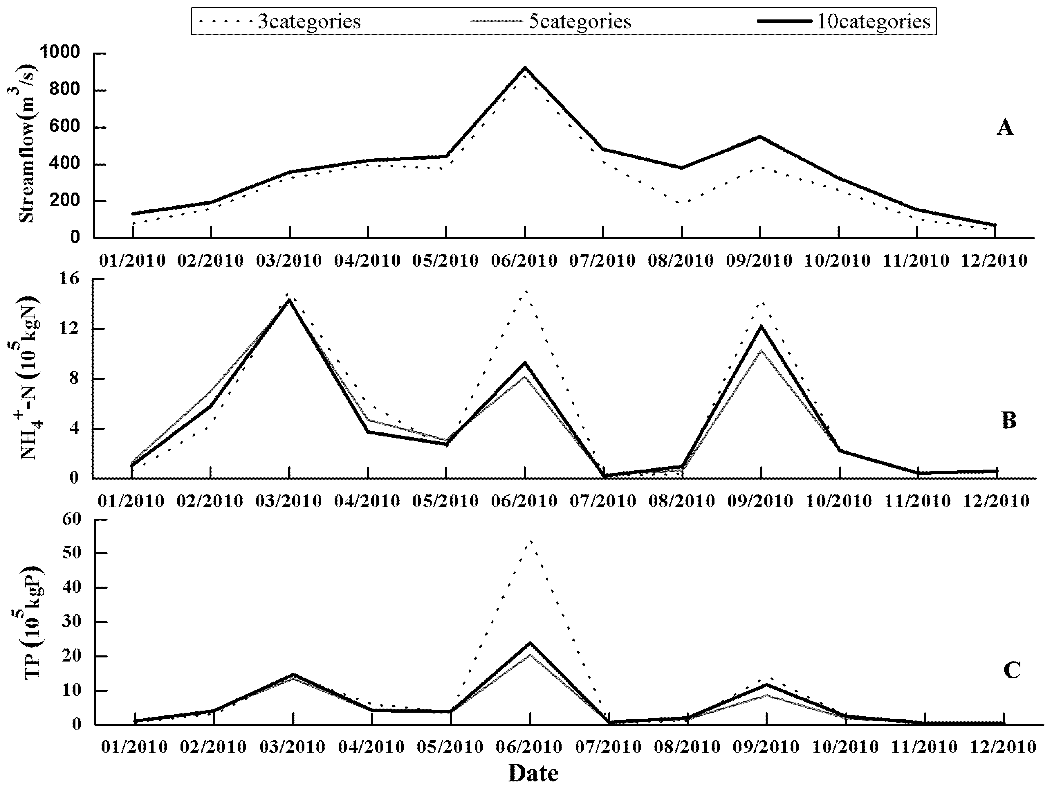
There were little differences in simulated streamflow using the three LULC datasets with ten, five and three categories. In contrast, significant differences in simulated monthly NH
4+-N and TP loads were exhibited when using these three LULC datasets with different levels of detail. When comparing LULC datasets from ten categories to those with five and three categories, the relative differences in predicted monthly NH
4+-N and TP loads were −6.6 to −6.5 % and −13.3 to −7.3 %, respectively (
Table 6 and
Figure 4).
The mean values of monthly and daily NH
4+-N and TP loads simulated were lower when using LULC datasets with three and five categories, compared to the simulation results using LULC datasets with ten categories (
Table 6). Aggregation can reduce potential map errors [
34], while it may result in a considerable loss of information [
16]. Therefore, it is understandable that an aggregation procedure, represented by more coarsely classified LULC datasets, resulted in lower mean values of monthly and daily NH
4+-N and TP loads simulated. However, such tendency showed somewhat seasonal variations. As shown in
Figure 4, monthly NH
4+-N and TP loads on June 2010 and September simulated using LULC data with three categories was significantly higher than those using LULC data with five and ten categories.
Table 6.
Comparison of simulation output with regards to streamflow, NH4+-N and TP loads when using three LULC datasets with different levels of classification.
Table 6.
Comparison of simulation output with regards to streamflow, NH4+-N and TP loads when using three LULC datasets with different levels of classification.
| | Streamflow (m3/s) | NH4+-N Load (× 103 kg N) | TP Load (× 103 kg P) |
|---|
| LULC Categories | 3 | 5 | 10 | 3 | 5 | 10 | 3 | 5 | 10 |
|---|
| Monthly mean | 300.98 | 302.26 | 301.65 | 532.74 | 531.95 | 569.49 | 817.06 | 764.32 | 881.72 |
| Changed amount | −0.67 | 0.61 | - | −36.75 | −37.54 | - | −64.66 | −117.40 | |
| Monthly Changed percentage (%) | −0.22 | 0.20 | - | −6.45 | −6.59 | - | −7.33 | −13.31 | |
| Daily mean | 300.42 | 301.66 | 301.12 | 17.51 | 17.49 | 18.72 | 26.86 | 25.13 | 28.99 |
| Daily Changed amount | −0.70 | 0.54 | - | −1.21 | −1.23 | - | −2.13 | −3.86 | - |
| Daily Changed percentage (%) | −0.23 | 0.18 | - | −6.46 | −6.57 | - | −7.35 | −13.31 | - |
Figure 4.
Comparisons among monthly streamflow (A), NH4+-N (B) and TP (C) loads predicted when using LULC datasets with three levels of detail.
Figure 4.
Comparisons among monthly streamflow (A), NH4+-N (B) and TP (C) loads predicted when using LULC datasets with three levels of detail.
Mean values of monthly and daily NH
4+-N and TP loads simulated using LULC data with five categories were lower than those using LULC data with three categories. This might have been caused by the different operations in the SWAT due to the aggregation effects of land use categories. In this study, when using LULC datasets with three categories in the SWAT model, we merged Forest, Barren and Water into “Natural”. Given that Forest has the typical characteristics of “Natural” because of the largest proportion of “Natural” and relatively less anthropogenic disturbance, the new category “Natural” was treated as Forest in the SWAT model. This process can be regarded as afforestation and may reduce streamflow as the higher water holding and conservation properties and evapotranspiration ability of forest [
35,
36,
37]. Therefore, monthly and daily streamflow predicted when using LULC datasets with three categories was a little lower than the simulated results using LULC data with five categories.
The categories high density residential area, low density residential area, industrial land and transportation were summarized as Built-up for LULC datasets with five and three categories, which was represented by a high density residential area in the SWAT model. Such similar operations may overestimate the role of ISA in urban areas, which could result in the higher values of the NH4+-N and TP loads simulated when using LULC datasets with ten categories, compared to the NH4+-N and TP loads simulated using LULC datasets with three and five categories.
Streamflow may increase with the finer classified LULC datasets [
38]. However, a watershed modeling analysis of urban catchments based on the SWMM model resulted in an opposite observation that using LULC datasets with coarser spatial resolution and a lower level of classification produces a higher runoff volume and TSS prediction [
1]. Comparing the LULC datasets with different levels of detail, there were no significant differences in monthly and daily streamflow predicted while coarser LULC datasets generally predicted lower monthly NH
4+-N and TP loads in this study. The underestimation of NH
4+-N and TP loads with the coarser LULC classification might lead to ignoring a water pollution emergency. Given that diffuse pollution sources and control measures are directly linked to land use, as well as the wide application of environment models for decision making, LULC datasets with different points in time and levels of details should be considered seriously for appropriate watershed assessment and management.
In this study, we developed two scenarios and used SWAT model which was calibrated and verified to evaluate the relative influence of different LULC datasets on watershed modeling. The simulation results didn’t show significant difference using LULC datasets with different points in time and levels of detail, especially for the streamflow simulation. On the one hand, LULC datasets maybe had little impact because there was little change in the LULC conditions over the study period. On the other hand, the specific operations regarding assigning parameter values to the combined category in the SWAT model system may influence the simulation results. In the next agenda, we need to improve the scenarios development for further model’s applications such as evaluating BMP’s implementation and assessing the effect of dam construction on water quantity and water quality. LULC data issue such as temporal mismatch of data, errors in LULC classification needs to be recognized when exploring the influence of LULC datasets on watershed modeling, which can made the data uncertainty propagated.


 is the mean of the dependent variable and Ŷi is the ith fitted value.
