A Two-Stage Approach for Medical Supplies Intermodal Transportation in Large-Scale Disaster Responses

Abstract
:1. Introduction
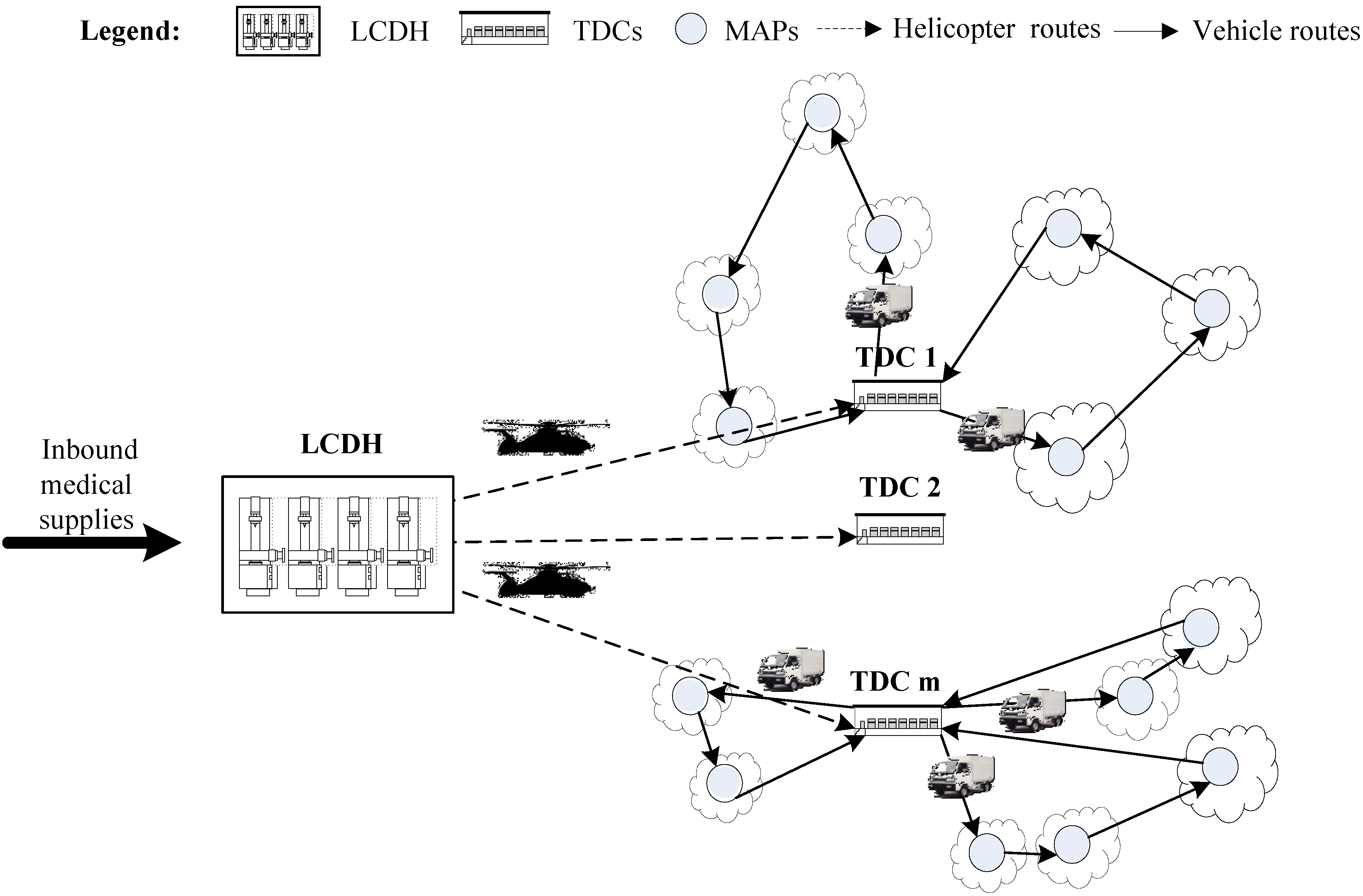
- Helicopters are not subject to existing transportation networks and can fly straight to affected areas, which could sharply shorten the delivery time of medical supplies.
- Helicopters can take off and land vertically at relatively small places. Thus, it is flexible and quick to select and clear up places as TDCs for receiving medical supplies from helicopters.
- In destructive disasters such as earthquakes and floods, the cut off of key roads often makes helicopters the most effective transportation mode to isolated affected areas.
2. Literature Review
3. The Proposed Approach
3.1. A Two-Stage Problem Formulation
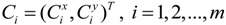 ;
;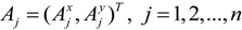 ;
; : The union of NCi and the ith TDC, whose index in the set is 0;
 : The number of the elements in , which is equal to nCi + 1;
 : The available load of vehicle k when the vehicle travels from the jth MAP (or the ith TDC) to the lth MAP (or the ith TDC),
 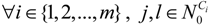 ;
; : The distance among the ith TDC and its covered MAPs, ;
 : A binary variable: = 1 means vehicle k travels from the jth MAP (or the ith TDC) to the lth MAP (or the ith TDC),
  ; otherwise = 0;
 : A binary variable: = 1 means that the jth MAP (or the ith TDC) is visited by vehicle k, ; otherwise, = 0.
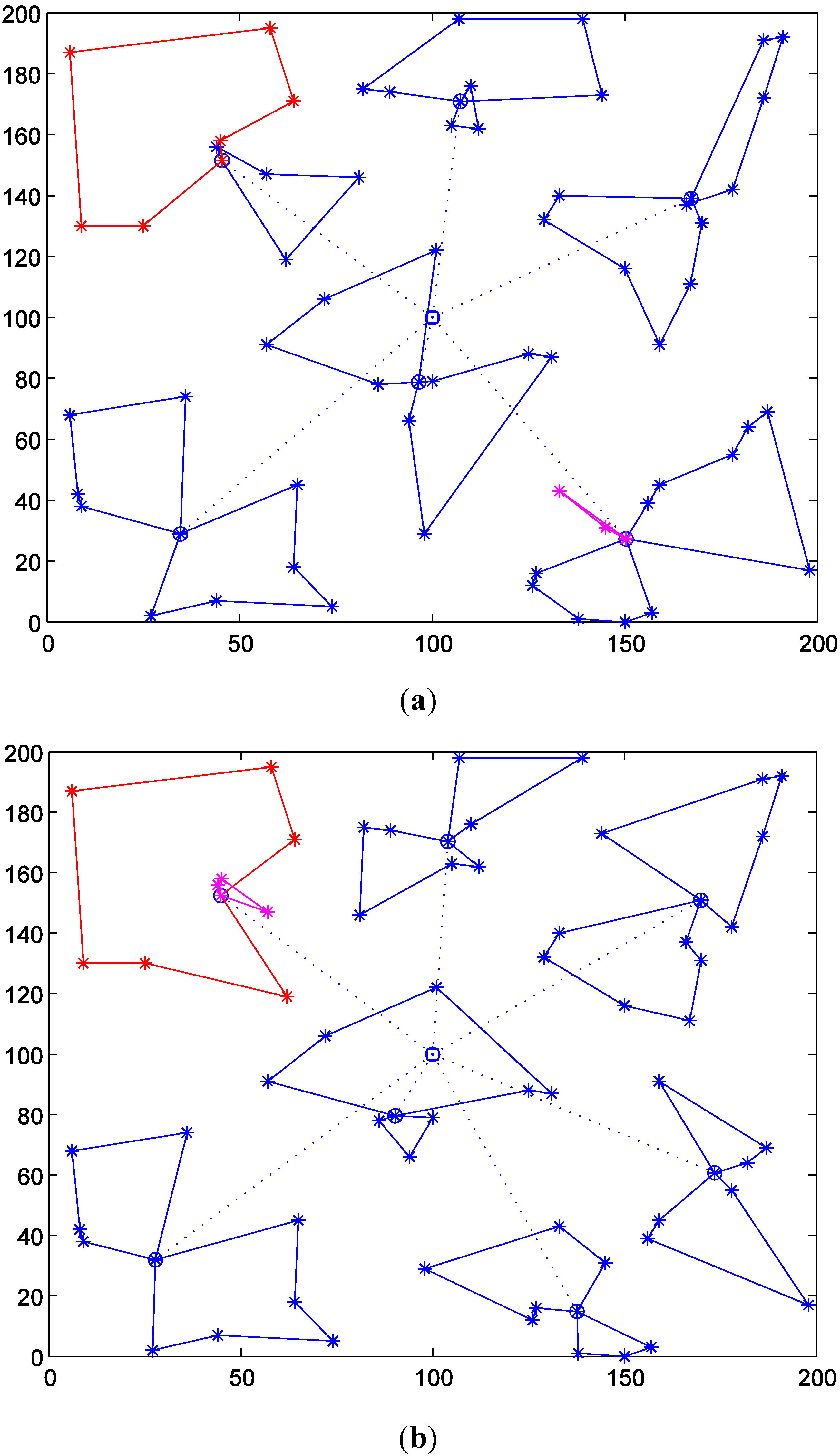
3.2. Stage I: Selecting TDCs and Assigning MAPs
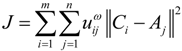
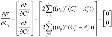
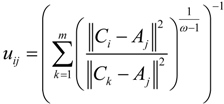
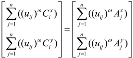
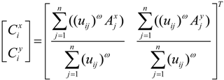
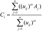
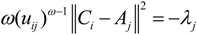
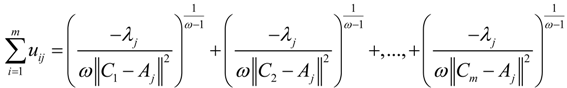
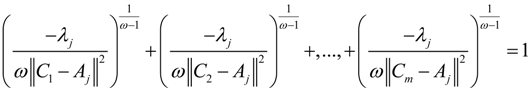
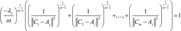
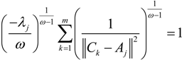
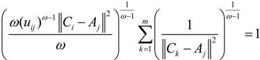
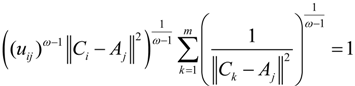
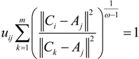
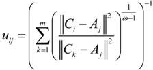
 represents the distance between Ci and Aj, that is,
 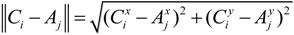 , and ω ∊ (1,∞) is a weighted coefficient. As we can see, if is smaller, a bigger weight
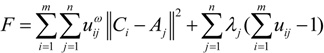
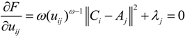
  will be assigned to it, so the solutions of Equation (2) (that is, Ci s) could produce the shortest total distance among TDCs and their covered MAPs., according to the Lagrange algorithm [23,24], the constrained objective Equation (2) could be transformed into the following unconstrained objective Equation:
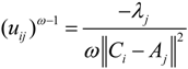
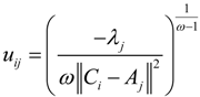
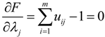
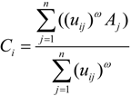
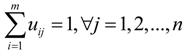
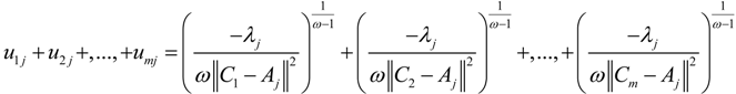
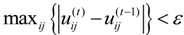 , where ε is a given threshold between 0 and 1, and t represents the iteration step. After getting the uij, we could assign the jth MAP to the TDC with the maximal uij = 1,2,…,m.
 : the location of selected TDCs; U(t) = [uij]m×n: the final membership degree matrix; J(t): the value of the objective function (2); NCi(t): The set of covered MAPs of TDC . (In details, we randomly generate the initial locations of m TDCs, and then use the normalized reciprocals of the distances among MAPs and the initial TDCs to determine the initial membership degrees);
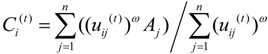 where t represents the iteration step to calculate thelocations of TDCs (i.e., , i = 1,2,…,m);
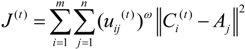 to get the value of the objective function; if , then stop the iteration and turn to Step 6 with the values of , U(t) and J(t);
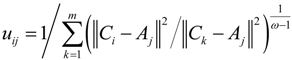 , then t = t + 1 and go to Step 3;, and judge the covered Aj s of each (i.e., NCi(t)); output , U(t), J(t) and NCi(t).
3.3. Stage II: Arranging Delivery Routes

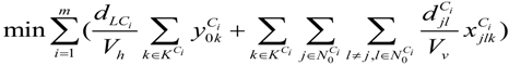
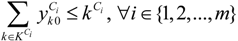
 denotes the number of used vehicles starting from the ith TDC, which is also equal to the number of vehicle routes from the ith TDC, so
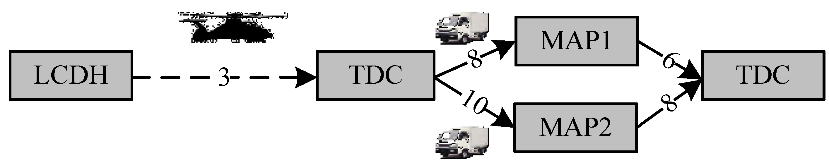
  denotes helicopter travel time considered in the intermodal duration time for MAPs covered by the ith TDC;
  denotes vehicle travel time considered in the intermodal duration time for MAPs covered by the ith TDC.
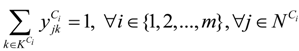
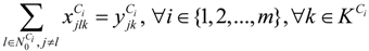
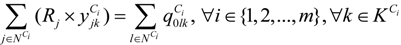


 represents the number of vehicles visiting the jth MAP.
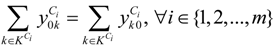
 ) is equal to the number of vehicles returning to the ith TDC (that is,
  ).
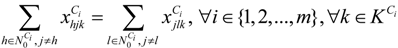
). represents the number of vehicles arriving at the jth MAP and
  represents the number of vehicles leaving from the jth MAP.
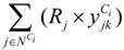 represents the total quantity of medical supplies allocated to MAPs served by vehicle k and
  represents the total load of vehicle k when leaving from the ith TDC.
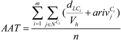
 represents the elapsed time from the ith TDC to the jth MAP. Note that the vehicle return time at TDCs is not included.
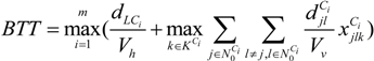
4. Numerical Experiments
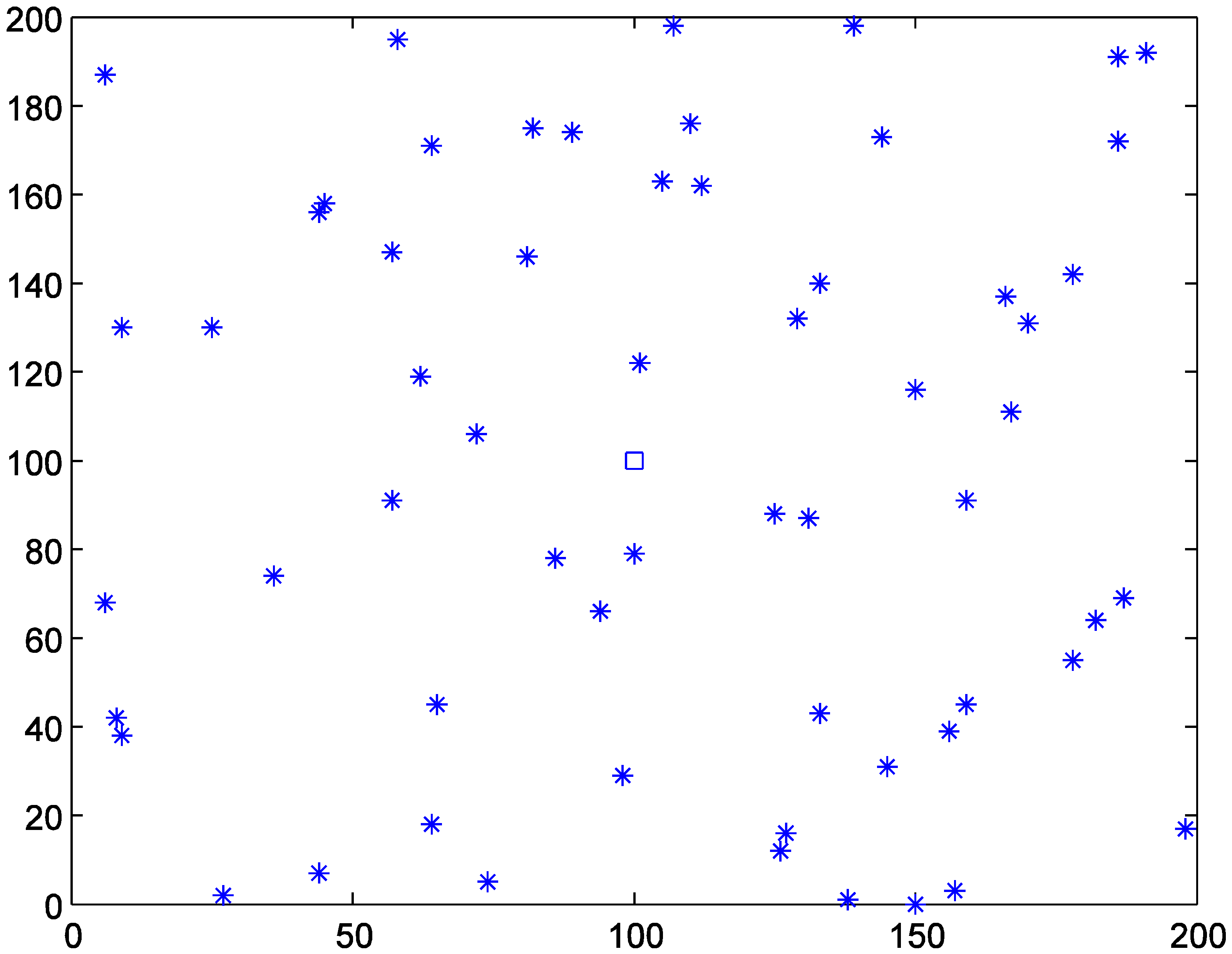
4.1. Data Generation

| MAPs |  |  | Rj | MAPs | | | Rj |
|---|---|---|---|---|---|---|---|
| 1 | 139 | 198 | 1136 | 31 | 44 | 156 | 880 |
| 2 | 57 | 91 | 1011 | 32 | 156 | 39 | 722 |
| 3 | 9 | 130 | 719 | 33 | 129 | 132 | 632 |
| 4 | 126 | 12 | 1026 | 34 | 170 | 131 | 737 |
| 5 | 144 | 173 | 721 | 35 | 94 | 66 | 1013 |
| 6 | 101 | 122 | 1055 | 36 | 167 | 111 | 880 |
| 7 | 157 | 3 | 1014 | 37 | 125 | 88 | 765 |
| 8 | 25 | 130 | 828 | 38 | 182 | 64 | 786 |
| 9 | 186 | 191 | 1039 | 39 | 6 | 187 | 495 |
| 10 | 72 | 106 | 974 | 40 | 110 | 176 | 753 |
| 11 | 112 | 162 | 654 | 41 | 100 | 79 | 832 |
| 12 | 159 | 45 | 831 | 42 | 44 | 7 | 1148 |
| 13 | 36 | 74 | 616 | 43 | 159 | 91 | 766 |
| 14 | 198 | 17 | 672 | 44 | 138 | 1 | 776 |
| 15 | 191 | 192 | 870 | 45 | 58 | 195 | 941 |
| 16 | 62 | 119 | 667 | 46 | 178 | 55 | 854 |
| 17 | 65 | 45 | 798 | 47 | 86 | 78 | 583 |
| 18 | 105 | 163 | 794 | 48 | 74 | 5 | 1129 |
| 19 | 131 | 87 | 886 | 49 | 8 | 42 | 1021 |
| 20 | 150 | 0 | 822 | 50 | 6 | 68 | 907 |
| 21 | 89 | 174 | 583 | 51 | 133 | 140 | 723 |
| 22 | 150 | 116 | 841 | 52 | 178 | 142 | 850 |
| 23 | 57 | 147 | 787 | 53 | 186 | 172 | 803 |
| 24 | 166 | 137 | 676 | 54 | 187 | 69 | 775 |
| 25 | 82 | 175 | 807 | 55 | 45 | 158 | 817 |
| 26 | 107 | 198 | 1119 | 56 | 98 | 29 | 926 |
| 27 | 9 | 38 | 808 | 57 | 133 | 43 | 824 |
| 28 | 64 | 18 | 882 | 58 | 145 | 31 | 1107 |
| 29 | 127 | 16 | 599 | 59 | 81 | 146 | 816 |
| 30 | 27 | 2 | 790 | 60 | 64 | 171 | 712 |
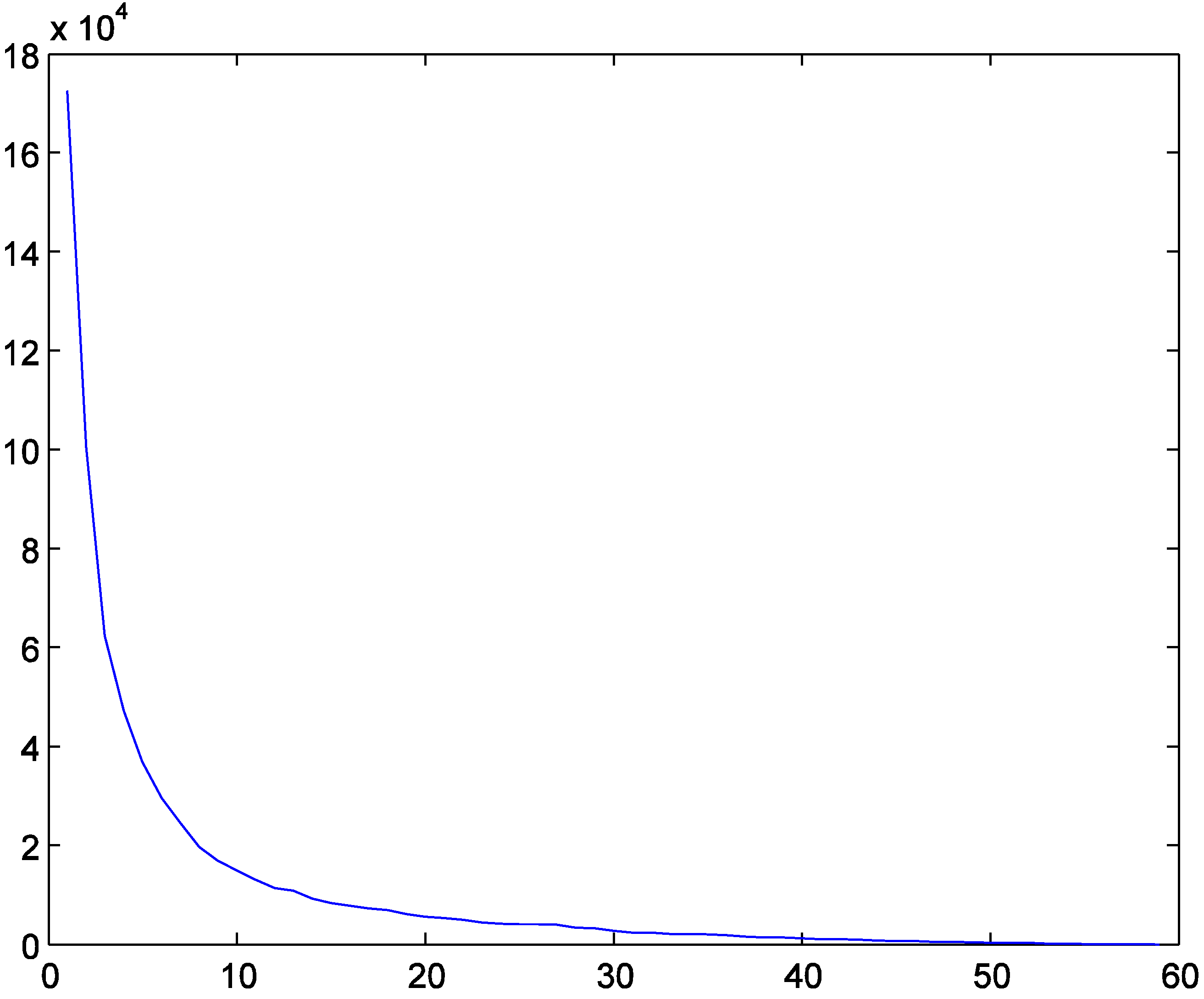
4.2. Results of Selected TDCs
| The Number of TDCs | The Selected Locations of TDCs | Iterations | The Value of Objective Equation (2) |
|---|---|---|---|
| 2 | (115.1215, 44.9284) (99.7824, 150.9591) | 41 | 172,532.3624 |
| 3 | (116.3484, 161.1088) (47.9796, 73.6059) (147.7658, 41.5159) | 91 | 100,417.3994 |
| 4 | (155.5038, 147.4673) (65.1837, 156.4479) (149.0295, 34.1258) (44.7962, 41.9201) | 43 | 62,411.0128 |
| 5 | (44.0622, 34.2492) (147.8524, 29.6506) (48.0010, 144.1700) (161.7073, 130.1246) (108.2454, 169.5621) | 80 | 47,221.8533 |
| 6 | (96.5021, 78.7748) (45.4646, 151.4802) (167.2060, 139.0513) (150.3087, 27.2637) (107.2651, 170.9193) (34.6524, 28.9273) | 62 | 36,831.0511 |
| 7 | (169.8822, 150.8263) (173.5107, 60.7168) (90.2298, 79.5935) (103.9641, 170.3261) (137.6201, 14.8587) (44.7909, 152.3732) (27.7608, 31.9316) | 78 | 29,522.1085 |
| 8 | (181.6705, 181.8142) (62.4966, 15.5558) (101.0444, 170.4035) (149.7739, 24.8483) (159.1980, 116.1517) (13.5109, 51.6327) (95.1028, 79.5795) (45.3501, 153.3287) | 57 | 24,550.5521 |
| 9 | (99.8256, 171.1113) (59.2840, 14.6074) (91.8373, 80.4970) (12.5390, 51.5439) (139.9251, 12.9395) (182.7777, 184.1032) (158.5230, 126.3868) (44.9873, 153.6155) (175.5131, 57.1305) | 53 | 19,631.8894 |
| 10 | (119.6735, 85.2224) (65.3041, 106.4243) (45.7608, 157.6658) (139.8517, 11.9312) (60.4220, 14.8274) (101.9682, 171.8361) (183.9530, 185.0312) (162.9210, 129.8682) (176.7298, 56.7747) (11.2449, 47.9950) | 100 | 16,907.0872 |
| 11 | (180.6445, 62.8425) (139.6802, 6.7262) (184.9137, 185.0973) (58.2463, 13.7295) (11.4684, 49.2855) (162.2845, 128.1690) (149.7515, 39.3025) (91.3246, 78.8456) (110.2706, 167.3838) (74.2499, 172.9312) (41.1820, 149.2225) | 73 | 14,917.4491 |
| 12 | (98.5393, 173.5782) (10.3469, 47.0838) (185.3382, 186.1472) (181.1156, 62.5890) (140.3170, 6.1505) (94.2870, 74.8852) (150.4305, 38.7289) (167.5805, 131.8681) (58.1328, 12.9601) (62.8250, 111.7601) (45.0970, 157.4632) (129.7547, 135.5699) | 79 | 12,977.8993 |
| 13 | (110.8082, 168.4445) (10.0571, 46.2019) (63.9118, 110.4021) (151.0760, 37.9474) (78.9164, 174.7529) (57.8343, 12.5276) (42.5859, 154.6934) (181.7441, 62.2657) (185.7684, 186.0645) (166.5562, 132.7123) (91.5287, 73.6481) (129.3355, 89.5669) (140.8238, 5.6172) | 58 | 11,382.4811 |
| 14 | (63.7141, 110.9293) (186.1755, 186.7686) (178.7301, 57.9741) (149.8187, 116.4298) (98.2565, 28.2879) (9.6585, 46.8682) (42.7754, 154.8233) (109.9915, 169.2300) (128.6312, 87.3772) (144.2500, 7.5919) (168.9176, 136.0067) (45.7029, 8.7246) (78.1378, 174.8745) (91.8098, 74.1798) | 73 | 10,761.5505 |
| 15 | (9.2761, 45.3432) (130.2494, 86.9024) (66.8312, 107.4951) (131.2589, 135.4988) (46.9954, 157.3454) (169.0423, 133.2947) (36.6269, 5.7054) (93.1979, 72.9595) (110.1389, 170.3292) (70.9212, 15.7676) (141.7105, 9.3871) (82.2789, 175.1017) (186.5786, 186.7270) (17.4716, 131.1668) (178.4745, 57.7653) | 57 | 9216.5779 |

4.3. Results of Delivery Routes
4.3.1. Results with Different Numbers of TDCs
| The Number of TDCs | Total Duration Time | Average Arrival Time | Biggest Traveling Time | Number of Used Helicopters | Number of Used Vehicles |
|---|---|---|---|---|---|
| 2 | 2236.33 | 101.69 | 286.75 | 2 | 12 |
| 3 | 2020.92 | 85.71 | 264.60 | 3 | 12 |
| 4 | 1896.19 | 93.79 | 226.22 | 4 | 12 |
| 5 | 1884.80 | 87.89 | 228.44 | 5 | 13 |
| 6 | 1759.45 | 80.78 | 217.16 | 6 | 13 |
| 7 | 1772.82 | 75.94 | 260.95 | 7 | 14 |
| 8 | 1746.35 | 80.62 | 260.51 | 8 | 15 |
| 9 | 1687.84 | 64.63 | 261.04 | 9 | 15 |
| 10 | 1681.97 | 73.04 | 232.67 | 10 | 16 |
| 11 | 1643.27 | 61.73 | 215.38 | 11 | 16 |
| 12 | 1615.44 | 63.80 | 233.26 | 12 | 15 |
| 13 | 1536.92 | 57.86 | 186.36 | 13 | 16 |
| 14 | 1512.55 | 64.16 | 186.01 | 14 | 16 |
| 15 | 1489.22 | 54.00 | 154.69 | 15 | 17 |
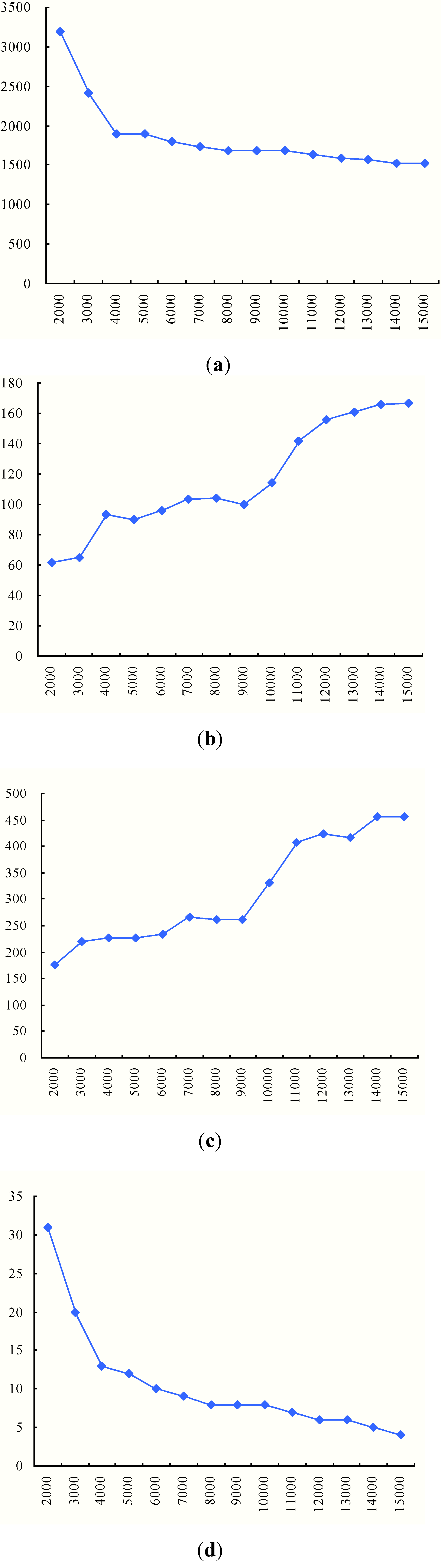
4.3.2. Results with Different Vehicle Maximum Capacities
| Vehicle Maximum Capacity | Total Duration Time | Average Arrival Time | Biggest Traveling Time | Number of Helicopters | Number of Vehicles |
|---|---|---|---|---|---|
| 2000 | 3191.10 | 62.00 | 175.09 | 4 | 31 |
| 3000 | 2406.51 | 64.96 | 220.32 | 4 | 20 |
| 4000 | 1893.31 | 93.58 | 226.89 | 4 | 13 |
| 5000 | 1900.70 | 89.71 | 226.89 | 4 | 12 |
| 6000 | 1798.74 | 96.05 | 233.14 | 4 | 10 |
| 7000 | 1728.03 | 103.63 | 266.03 | 4 | 9 |
| 8000 | 1683.76 | 104.21 | 261.21 | 4 | 8 |
| 9000 | 1684.34 | 99.59 | 261.21 | 4 | 8 |
| 10,000 | 1679.68 | 113.86 | 331.20 | 4 | 8 |
| 11,000 | 1636.28 | 141.39 | 408.06 | 4 | 7 |
| 12,000 | 1584.49 | 156.00 | 422.82 | 4 | 6 |
| 13,000 | 1565.34 | 160.76 | 416.06 | 4 | 6 |
| 14,000 | 1529.67 | 165.57 | 455.03 | 4 | 5 |
| 15,000 | 1515.92 | 166.57 | 455.03 | 4 | 4 |

4.3.3. Results with Different Helicopter Travel Speeds
| Helicopter Traveling Speeds | Total Duration Time | Average Arrival Time | Biggest Traveling Time | Number of Helicopters | Number of Vehicles |
|---|---|---|---|---|---|
| 1 | 2710.51 | 161.40 | 287.49 | 4 | 12 |
| 2 | 2258.11 | 123.84 | 252.75 | 4 | 12 |
| 3 | 2107.31 | 111.32 | 241.70 | 4 | 12 |
| 4 | 2031.91 | 105.06 | 236.17 | 4 | 12 |
| 5 | 1986.67 | 101.30 | 232.85 | 4 | 12 |
| 6 | 1956.51 | 98.79 | 230.64 | 4 | 12 |
| 7 | 1934.97 | 97.01 | 229.06 | 4 | 12 |
| 8 | 1918.81 | 95.66 | 227.88 | 4 | 12 |
| 9 | 1906.24 | 94.62 | 226.96 | 4 | 12 |
| 10 | 1896.19 | 93.79 | 226.22 | 4 | 12 |

5. Conclusions
Acknowledgments
Author Contributions
Conflicts of Interest
References
- Sheu, J.B. An emergency logistics distribution approach for quick response to urgent relief demand in disasters. Trans. Res. Pt. E Logist. Trans. Rev. 2007, 43, 687–709. [Google Scholar]
- Ruan, J.; Wang, X.; Shi, Y.; Sun, Z. Scenario-based path selection in uncertain emergency transportation networks. Int. J. Innov. Comput. I. 2013, 9, 3293–3305. [Google Scholar]
- Wang, D.; Qi, C.; Wang, H.W. Improving emergency response collaboration and resource allocation by task network mapping and analysis. Saf. Sci. 2014, 70, 9–18. [Google Scholar]
- Simpson, N.C.; Hancock, P.G. Fifty years of operational research and emergency response. J. Oper. Res. Soc. 2009, 60, S126–S139. [Google Scholar]
- Caunhye, A.M.; Nie, X.; Pokharel, S. Optimization models in emergency logistics: A literature review. Socio-Econ. Plan. Sci. 2012, 46, 4–13. [Google Scholar]
- Galindo, G.; Batta, R. Review of recent developments in OR/MS research in disaster operations management. Eur. J. Oper. Res. 2013, 230, 201–211. [Google Scholar]
- Jia, H.Z.; Ordóñez, F.; Dessouky, M.M. Solution approaches for facility location of medical supplies for large-scale emergencies. Comput. Ind. Eng. 2007, 52, 257–276. [Google Scholar]
- Mete, H.O.; Zabinsky, Z.B. Stochastic optimization of medical supply location and distribution in disaster management. Int. J. Prod. Econ. 2010, 126, 76–84. [Google Scholar]
- An, S.; Cui, N.; Li, X.; Ouyang, Y. Location planning for transit-based evacuation under the risk of service disruptions. Trans. Res. Part B Methodol. 2013, 54, 1–16. [Google Scholar]
- Yarmand, H.; Ivy, J.S.; Denton, B.; Lloyd, A.L. Optimal two-phase vaccine allocation to geographically different regions under uncertainty. Eur. J. Oper. Res. 2014, 233, 208–219. [Google Scholar]
- Haghani, A.; Oh, S.C. Formulation and solution of a multi-commodity, multi-modal network flow model for disaster relief operations. Trans. Res. Pt. A Policy Pract. 1996, 30, 231–250. [Google Scholar]
- Barbarosolu, G.; Arda, Y. A two-stage stochastic programming framework for transportation planning in disaster response. J. Oper. Res. Soc. 2004, 55, 43–53. [Google Scholar]
- Özdamar, L. Emergency logistics planning in natural disasters. Ann. Oper. Res. 2004, 129, 218–219. [Google Scholar]
- Hu, Z.H. A container multimodal transportation scheduling approach based on immune affinity model for emergency relief. Expert Syst. Appl. 2011, 38, 2632–2639. [Google Scholar]
- Najafi, M.; Eshghi, K.; Dullaert, W. A multi-objective robust optimization model for logistics planning in the earthquake response phase. Trans. Res. Pt. E Logist. Trans. Rev. 2013, 49, 217–249. [Google Scholar]
- Najafi, M.; Eshghi, K.; de Leeuw, S. A dynamic dispatching and routing model to plan/re-plan logistics activities in response to an earthquake. OR Spectr. 2014, 36, 323–356. [Google Scholar]
- Kovács, G.; Spens, K.M. Humanitarian logistics in disaster relief operations. Int. J. Phys. Distrib. Logist. Manage. 2007, 37, 99–114. [Google Scholar]
- Huang, M.; Smilowitz, K.; Balcik, B. Models for relief routing: Equity, efficiency and efficacy. Trans. Res. Part E Logist. Trans. Rev. 2012, 48, 2–18. [Google Scholar]
- Özdamar, L.; Demir, O. A hierarchical clustering and routing procedure for large scale disaster relief logistics planning. Trans. Res. Pt. E Logist. Trans. Rev. 2012, 48, 591–602. [Google Scholar]
- Sheu, J.B. Dynamic relief-demand management for emergency logistics operations under large-scale disasters. Trans. Res. Pt. E Logist. Trans. Rev. 2010, 46, 1–17. [Google Scholar]
- Abounacer, R.; Rekik, M.; Renaud, J. An exact solution approach for multi-objective location—Transportation problem for disaster response. Comput. Oper. Res. 2014, 41, 83–93. [Google Scholar]
- Barbarosoglu, G.; Özdamar, L.; Cevik, A. An interactive approach for hierarchical analysis of helicopter logistics in disaster relief operations. Eur. J. Oper. Res. 2002, 140, 118–133. [Google Scholar]
- Hestenes, M.R. Multiplier and gradient methods. J. Optim. Theory Appl. 1969, 4, 303–320. [Google Scholar]
- Fakhrzad, M.B.; Zare, H.K. Combination of genetic algorithm with Lagrange multipliers for lot-size determination in multi-stage production scheduling problems. Expert Syst. Appl. 2009, 36, 10180–10187. [Google Scholar]
- Wang, X.; Ruan, J.; Shi, Y. A recovery model for combinational disruptions in logistics delivery: Considering the real-world participators. Int. J. Prod. Econ. 2012, 140, 508–520. [Google Scholar]
Appendix I. The Derivation of Equation (7)
Appendix II. The Derivation of Equation (8)
 into the above formula, we can get:
© 2014 by the authors; licensee MDPI, Basel, Switzerland. This article is an open access article distributed under the terms and conditions of the Creative Commons Attribution license (http://creativecommons.org/licenses/by/4.0/).
Share and Cite
Ruan, J.; Wang, X.; Shi, Y. A Two-Stage Approach for Medical Supplies Intermodal Transportation in Large-Scale Disaster Responses. Int. J. Environ. Res. Public Health 2014, 11, 11081-11109. https://doi.org/10.3390/ijerph111111081
Ruan J, Wang X, Shi Y. A Two-Stage Approach for Medical Supplies Intermodal Transportation in Large-Scale Disaster Responses. International Journal of Environmental Research and Public Health. 2014; 11(11):11081-11109. https://doi.org/10.3390/ijerph111111081
Chicago/Turabian StyleRuan, Junhu, Xuping Wang, and Yan Shi. 2014. "A Two-Stage Approach for Medical Supplies Intermodal Transportation in Large-Scale Disaster Responses" International Journal of Environmental Research and Public Health 11, no. 11: 11081-11109. https://doi.org/10.3390/ijerph111111081