1. Introduction
Air pollution exposure assessment is a crucial component to investigate the relationship between air pollution and health effects in epidemiological studies. As the magnitude of the health effects of ambient air pollution often relies on exposure assessment methods, the method for estimating exposure is an important factor to determine the actual or potential exposure level of humans. The most desirable method for estimating personal exposure is to measure directly through personal monitoring [
1]. However, since direct measurement of exposure at the individual level can be time consuming and expensive, in large-scale epidemiological studies it can be commonly estimated by fixed ambient air pollution monitoring data. Also, most epidemiology studies use data spatially aggregated at the area level because of data limitations.
The advantage of monitoring data includes the ability to use existing data and to cover a large spatial area [
2]. Previous epidemiological studies for air pollution have assigned exposures using data from a few nearest air monitors and used the exposure as a surrogate for the actual personal exposure [
3,
4]. However, this approach may cause uncertainty such as exposure misclassification, and may underestimate or overestimate the health effects of air pollution because it does not reflect the spatial heterogeneity of individuals [
5,
6].
Recently, spatial interpolation is increasingly being used to assess adverse health effects associated with environmental risk factors. Advances in geostatistical methods and geospatial technologies based on geographic information systems (GIS) have made it possible to improve air pollution exposure assessments. Specifically, a number of studies have been conducted to estimate the relationship between air pollution and health outcomes using spatial methods such as proximity models [
7,
8], geostatistical methods [
9,
10] and land-use regression models [
11,
12]. In particular, to minimize exposure misclassification, advanced interpolation methods have been applied to better estimate a population’s or individual’s exposures to air pollution. Kriging is one of these interpolation methods, which is developed based on statistical techniques in geostatistics for optimal spatial prediction at unobserved locations [
13,
14].
The short-term exposure effects of ozone have been demonstrated to cause lung function impairment, lung inflammation and respiratory symptoms [
15]. In addition, high O
3 concentrations have been associated with adverse effects on respiration and lung function [
16]. While many studies have focused on the characteristics of surface ozone concentration and distribution, relatively few have investigated how this pollutant affected health outcomes. Also, almost no investigations have utilized improved methods for estimating exposure for the association between ozone and health outcomes.
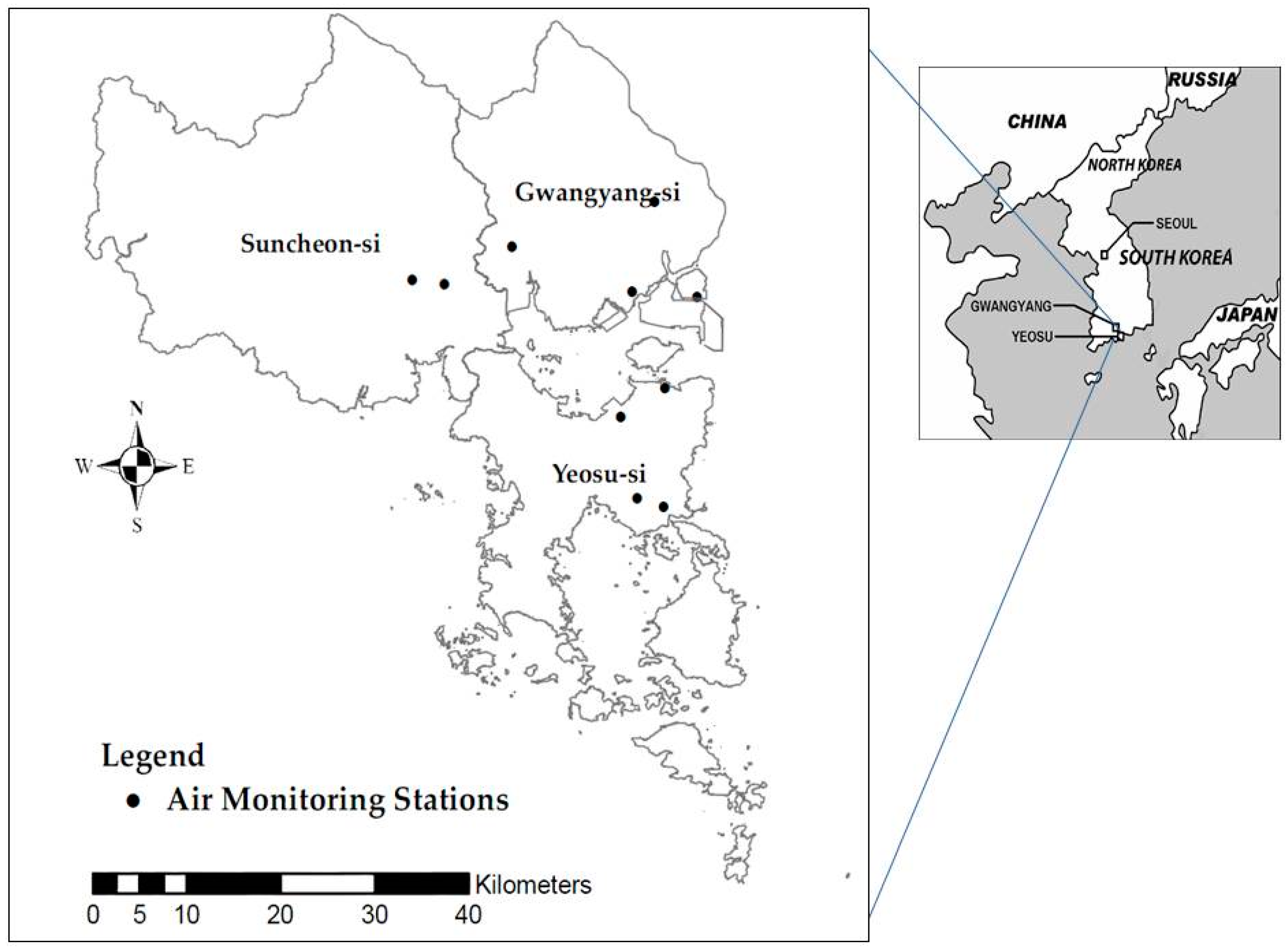
In this study, we investigated the association between ozone level at an industrial complex in South Korea and lung function with two objectives, one of which is estimating and comparing ozone exposures using four different methods including simple averaging across all monitors in the study area, spatial interpolation by the nearest monitoring station, inverse distance weighting and ordinary kriging and the other of which is evaluating how different methods for estimating exposure influence health outcomes.
3. Results
A total of 2283 ozone exposures were estimated at the individual level from information based on the residential locations of the subjects. The summary descriptive statistics of O
3 concentrations for each method are shown in
Table 1.
These summary statistics are the average across the 2283 subjects. The mean O
3 values were 42.2 ppb from Method 1, 40.9 from Method 2, 41.4 from Method 3 and 41.7 from Method 4. The average values of estimated O
3 exposures were not significantly different in each method. The largest variation in spatial concentration among the four methods was nearest the monitors (Method 2).
Table 2 shows the mean and range levels of daily max 8 h moving average of O
3 concentrations on each day, and the lung function test was performed for 1 lag, 2 lag, 0–1 lag, 1–2 lag and 0–2 lag by the four different methods for estimating exposure.
Ranges of concentrations of ozone were 28.3–85.9 ppb (Method 1), 24.0–96.4 (Method 2), 24.0–93.9 (Method 3), 23.9–98.2 (Method 4). The concentrations of ozone on the day of the lung function test (0d) were the highest in all methods except for Method 2 (nearest monitor). We found that the estimated ozone exposure from kriging showed more excellent cross-validation results than those from the other interpolation methods from the cross-validation analysis. The RMSE indicated the difference between observed and predicted ozone concentration for kriging was the lowest. The COD value for kriging was less than those of nearest monitor and IDW (
Table 3).
A summary statistic of the demographic characteristics and lung function measurements of the study populations is presented in
Table 4. The mean age of subjects was 41.8 year, and 56.9% were female. The mean FVC and FEV
1 of each age group were 2.26, 1.92 in children, 3.23, 2.69 in adults and 2.39, 1.82 in the elderly, respectively (
Table 4).
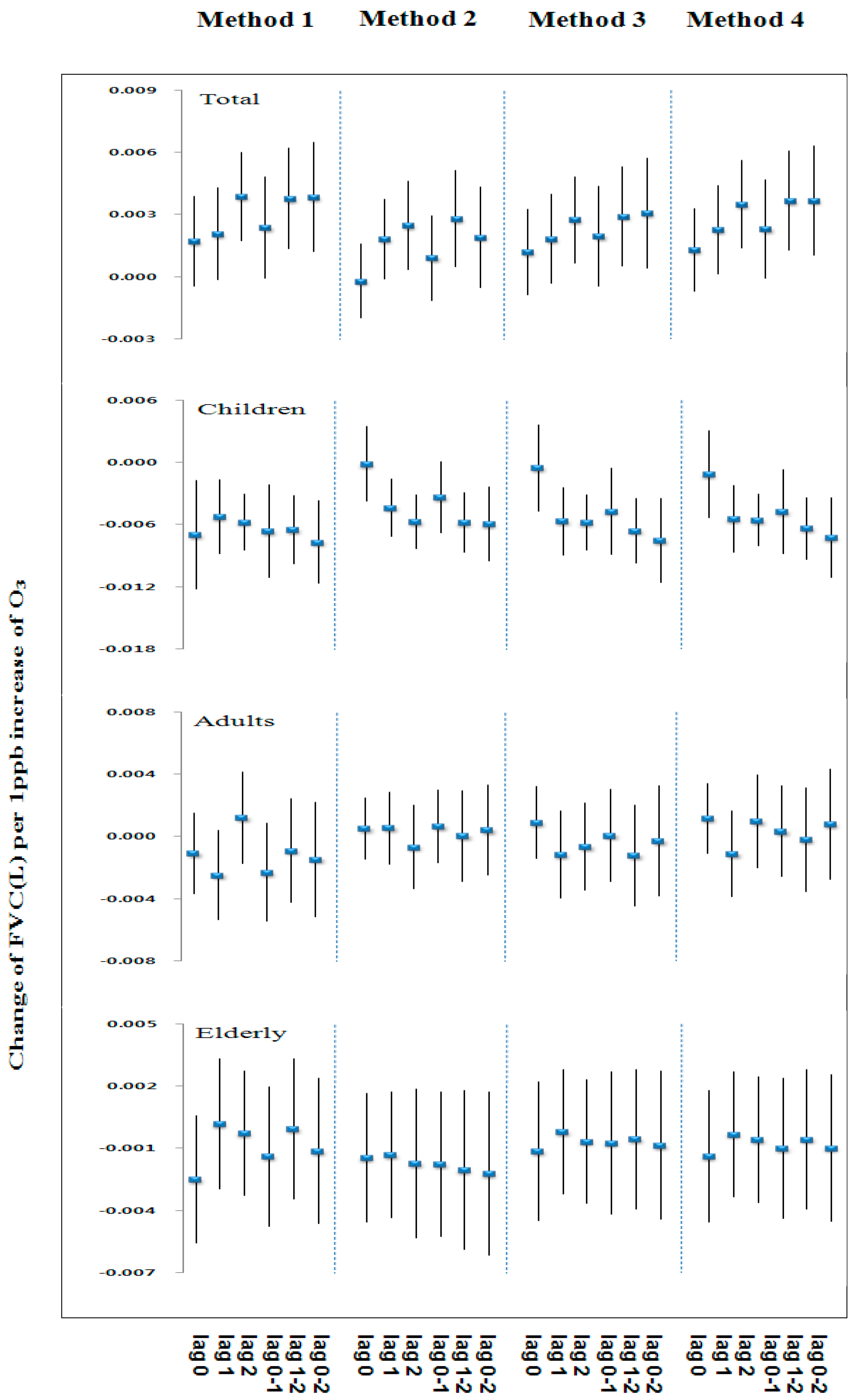
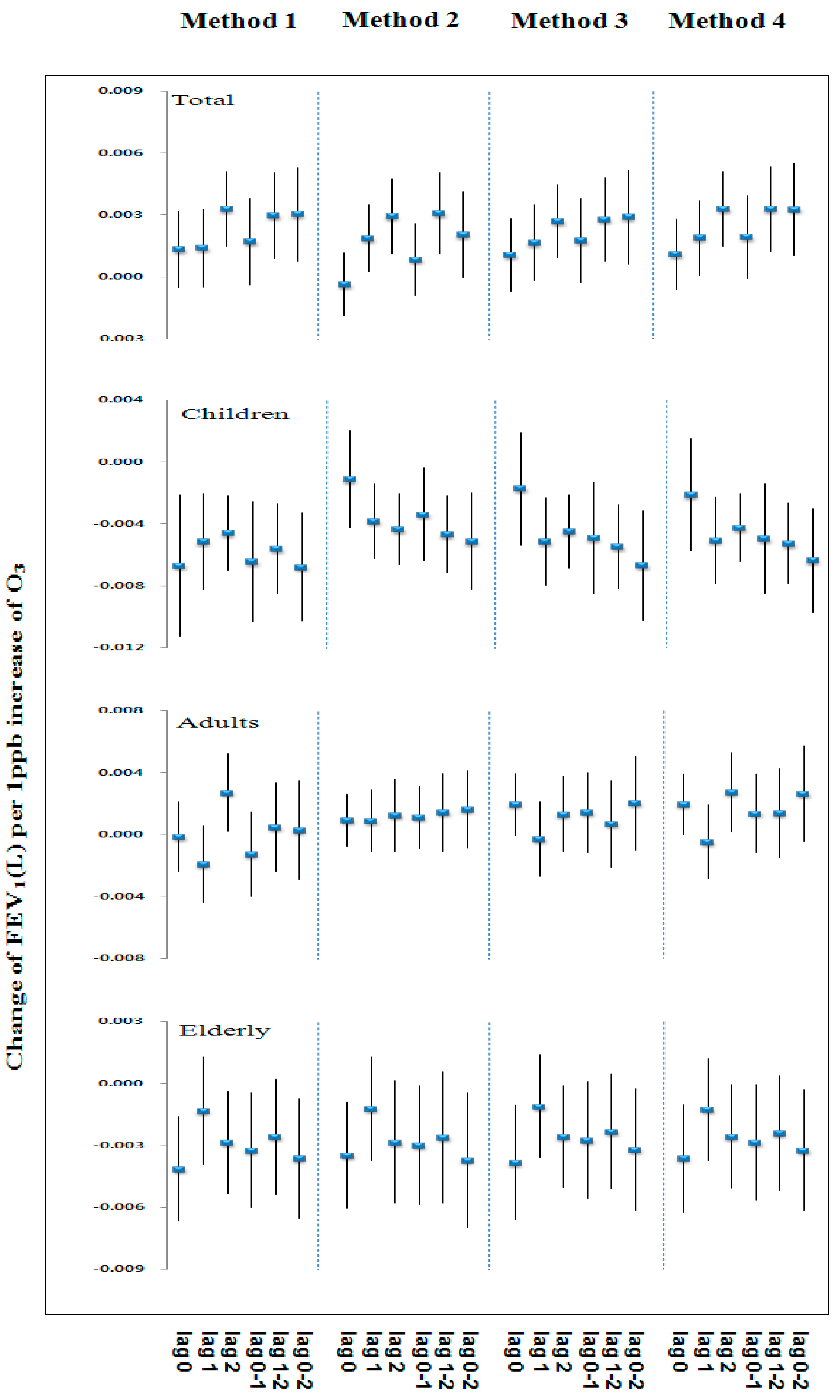
Figure 2 and
Figure 3 show similar patterns of changes in effect size on FVC and FEV
1 associated with exposure to 1 ppb increase of ozone concentrations by lag and the four methods for estimating exposure in each age group. The overall change of effect size on lung function in each age group tended to show similar patterns for lag and the methods for estimating exposure.
Table 5 and
Table 6 show the estimated changes in FVC and FEV
1 for an increase to the inter-quartile range of O
3 concentrations by the four methods and age groups. In children (age 9–14), the significant negative association were observed between O
3 and FVC and FEV
1 for most of the lag and the methods.
The largest effect of O3 was found at the average of the lung function for the test day and last 2 days (0–2 days). In adult (age 15–64), the effect of O3 on reduction in FVC and FEV1 were not significant for any lag and the methods. In the elderly (age ≥ 65), the negative association between FEV1 and O3 was significant except on 0 day, 0–1 day, but FVCs were not significant for any lag and the methods.
4. Discussion
This study assessed the association between ozone exposure and lung function using four methods for estimating exposure. To minimize exposure misclassification, we tried to estimate more accurate exposure levels by using the spatial analysis technique in the exposure assessment of epidemiological studies. Although other researchers have employed a similar method to estimate individual levels of exposure to air pollution, they did not use such approaches to compare the lung function effects of ozone in different age groups [
25,
26,
27]. In addition, no investigations have been done utilizing interpolation methods for estimating exposure to identify the association between ozone and health outcomes in Gwangyang Bay.
In this study, we developed better exposure estimates through the application of a kriging method among the four interpolation methods. Previous studies with the application of interpolation methods have suggested the similar associations. A study by Son et al. predicted individual levels of exposure to air pollution using the four different approaches (average across all monitors, nearest monitor, IDW and kriging) to identify the association between air pollution and lung function [
28]. They found that the kriging method provided the most accurate estimates of exposures, and the magnitudes of health effect estimates were generally higher when using exposures based on averaging across all monitors or kriging. A simulation study by Kim et al. examined exposure prediction approaches such as the nearest monitor and kriging methods for PM
2.5 affecting relative risk estimates for cardiovascular events in Los Angeles [
29]. Their findings indicated that a kriging method provided more accurate exposure estimates because it had smaller average mean square prediction error. Liao et al. reported that daily kriging estimations of residential−level ambient PM concentrations were feasible on a national scale [
21]. Jerrett et al. suggested that the health effects associated with exposure to PM
2.5 were approximately three times greater using the kriging approach than using the average ambient concentration approach previously employed in the American Cancer Society (ACS) cohort. This can be explained by the fact that the exposure estimation method used in estimating air pollution exposure may affect the results of epidemiologic studies [
25]. However, there have been debates on which methods are most suitable for estimating air pollution from ambient monitors.
The advantage of regulatory monitoring network data includes the ability to use existing data and to estimate individual level exposure. This monitoring data would allow studies on the relationship between air pollution and health outcomes for times, locations, and pollutants for which monitoring data are limited or unavailable [
2]. The Ministry of Environment (MOE) in Korea has generated hourly ambient air concentration data from 257 urban air quality monitors, including O
3, PM
10, NO
2, SO
2 and CO [
30]. This monitoring network data provide good temporal resolutions, with hourly monitor coverage of 0.003 monitor/km
2 at a national scale. Air monitoring stations have typically been installed in urban areas where population density is high [
2,
31]. For instance, the most densely populated Seoul, the capital of Korea, had hourly monitor coverage of 0.04 monitor/km
2. Although fewer monitors were available in our study area, monitor coverage had a high spatial resolution of 0.01 monitor/km
2.
Declines in FVC and FEV
1 were significantly associated with ozone concentration in children. In this study, we assessed the relationship between changes in lung function and ozone exposure as estimated by the interpolation method. The results of this study show that there were no significant associations between ozone exposure and lung function in the whole subject, but a decrease in lung function was observed in children for most of the lag and methods. More specifically, the declines in FVC and FEV
1 were significantly associated with most of the lag and methods, and the largest effect was observed for 0–2 days. Previous researches of decrease in lung function on O
3 exposure in children have demonstrated similar results [
32,
33,
34,
35]. According to Chang et al., 1 ppb increase in O
3 was significantly associated with decreased FVC 2.29 mL among 2919 students who lived in five school districts in Taipei [
36]. Significant lag effects were observed in FVC for 0 day, 1 day and 2 days before the spirometry test. Son et al. reported that a 11 ppb increase (IQR) in O
3 was associated with a decrease of 6.1% (95% confidence interval, 5.0% to 7.3%) in FVC and 0.5% (95% confidence interval, 0.03% to 0.96%) in FEV
1 in lag 0–2 day, based on kriging exposures [
28]. Moreover, ozone exposure is well documented in many studies to cause adverse lung injury effects, including reduced lung capacity, chronic obstructive pulmonary disease, and severe asthma exacerbation [
37,
38]. In this study, ozone level was calculated as the maximum daily 8-h moving average. The maximum daily 8-h moving average was computed by selecting the highest value among 17 daily 8-h moving average. Since lung function tests were performed in the morning, estimated ozone level for the lung function test day (0 day) may have implications for interpreting the association between ozone level and lung function.
It is well established that ground-level ozone is generated from the photochemical oxidation of NO
x emissions and volatile organic compounds (VOCs). The major sources of NO
x and VOCs are emitted during fuel combustion from automobiles, fossil fuel power plants and industrial processing. Our study area was a major industrial hub in Korea, which may release a wide range of air pollutants into the atmosphere. These air pollutants may affect the respiratory health of communities living close to the industrial areas. In particular, children are potentially more vulnerable than adults to environmental risk factors like air pollution. Unlike adults, the children’s respiratory system is constantly growing and they breathe more air than adults do, in proportion to their weight. During the stages of rapid growth, immature lungs may be the most susceptible [
33,
39,
40]. Several studies have demonstrated the association between respiratory health such as asthma and lung function in children and proximity to petrochemical sites [
41,
42,
43]. According to the study of Rusconi et al. children living in a petrochemical polluted area (Sarroch) versus a reference area (Burcei) showed a decrease in lung function (variation in FEV
1 = −10.3% (90% CI = −15.0 to −6.0%)) [
43].
To improve the accuracy and better reflect the linkages between air pollution and health outcomes, multiple methods for estimating exposure to ambient ozone were used. Use of spatial interpolation methods may be useful in providing individual-level exposures for locations without monitors and alternative for epidemiological analyses at the individual-level on the health effects. However, these approaches can contribute to uncertainty in estimating exposure, including monitoring site location, distance between a monitor and population, time-activity patterns of residents, and methodological choices. Because people spend more time indoors than outdoors, exposure misclassification bias can occur. For example, the average time spent per day in residential indoors was over 50% in 24 hours a day [
44,
45,
46]. Thus, information on time spent in each micro-environment should be used in assessing actual personal exposures.


 ,
, 


