Appendix A
Equilibrium solutions of supply chains under different decision scenarios are calculated and presented in the following context below.
Appendix A.1. Solutions under Scenario NN
By solving , we can derive . The demand functions of the two retailers are and .
The profits of the two manufacturers and two retailers can be modeled as follows based on the previously presented demand functions:
By solving equations and , we can obtain the following optimal functions: and .
After substituting the function of
and
into
and
and solving equations
and
, we can derive:
By substituting and into the equations about and , we can derive
By substituting and into the equations on and , we can obtain
By substituting the optimal solution into the equations about profits of the two manufacturers and two retailers, we can obtain
Equilibrium solutions under scenario NN are summarized and presented in
Table A1.
Table A1.
Equilibrium outcomes under scenario NN.
Table A1.
Equilibrium outcomes under scenario NN.
| Scenario NN | Supply Chain 1 | Supply Chain 2 |
|---|
| | |
| | |
| | |
| | |
| | |
Appendix A.2. Solutions under Scenario NL
By solving , we can derive . The demand functions of the two retailers are as follows: and .
The profits of the two manufacturers and two retailers can be modeled as follows based on the previously presented demand functions:
By solving equations
and
, we can obtain the following optimal functions:
After substituting the function of and into and and solving equations and , we can derive
By substituting and into the equations about and , we can derive
By substituting and into the equations on and , we can obtain
By substituting the optimal solution into the equations about profits of the two manufacturers and two retailers, we can obtain the following equations:
We summarize equilibrium solutions under scenario NL and presented in
Table A2.
Table A2.
Equilibrium outcomes under scenario NL.
Table A2.
Equilibrium outcomes under scenario NL.
| Scenario NL | Supply Chain 1 | Supply Chain 2 |
|---|
| | |
| | |
| | |
| | |
| | |
Appendix A.3. Solutions under Scenario LN
By solving
, we can derive
. The demand functions of the two retailers are as follows:
The profits of the two manufacturers and two retailers can be modeled as follows based on the previously presented demand functions:
By solving equations and , we can obtain the optimal functions
After substituting the function of and into and and solving equations and , we can derive
By substituting and into the equations about and , we can derive
By substituting and into the equations on and , we can obtain
By substituting the optimal solution into the equations about profits of the two manufacturers and two retailers, we can obtain the following equations:
Equilibrium solutions under scenario LN are summarized and presented in
Table A3.
Table A3.
Equilibrium outcomes under scenario LN.
Table A3.
Equilibrium outcomes under scenario LN.
| Scenario LN | Supply Chain 1 | Supply Chain 2 |
|---|
| | |
| | |
| | |
| | |
| | |
Appendix A.4. Solutions under Scenario LL
By solving
, we can derive
. The demand functions of the two retailers are as follows:
The profits of the two manufacturers and two retailers can be modeled as follows based on the previously presented demand functions:
By solving equations and , we can obtain the optimal functions and .
After substituting the function of and into and and solving equations and , we can derive
By substituting and into the equations about and , we can derive
By substituting and into the equations on and , we can obtain
By substituting the optimal solution into the equations about profits of the two manufacturers and two retailers, we can obtain the following equations:
We summarize equilibrium solutions under scenario LL and presented in
Table A4.
Table A4.
Equilibrium outcomes under scenario LL.
Table A4.
Equilibrium outcomes under scenario LL.
| Scenario LL | Supply Chain 1 | Supply Chain 2 |
|---|
| | |
| | |
| | |
| | |
| | |
Next, we analyze the choice of manufacturers.
Table A5 lists the equilibrium profit between manufacturers 1 and 2 under the four scenarios.
Table A5.
Equilibrium profit of the two manufacturers under the four scenarios.
Table A5.
Equilibrium profit of the two manufacturers under the four scenarios.
| | NN | NL | LN | LL |
|---|
| M1 | | | | |
| M2 | | | | |
Appendix B
Appendix B contains the proofs of the propositions and lemmas stated in the text.
Proof of Proposition 1. Due to , , and , we can derive ; thus, .
Manufacturer 1’s profit gap between scenario NN and scenario LN is
Due to , , , we can derive ,
When , . Thus, .
In the same manner, we can determined that when , .
Thus, if , regardless of what manufacturer 2 chooses to produce, then manufacturer 1 will choose to produce regular products.
In the same manner, we can determine that when , ; when , . This finding means that if , regardless of what manufacturer 1 chooses to produce, then manufacturer 2 will choose to produce regular products.
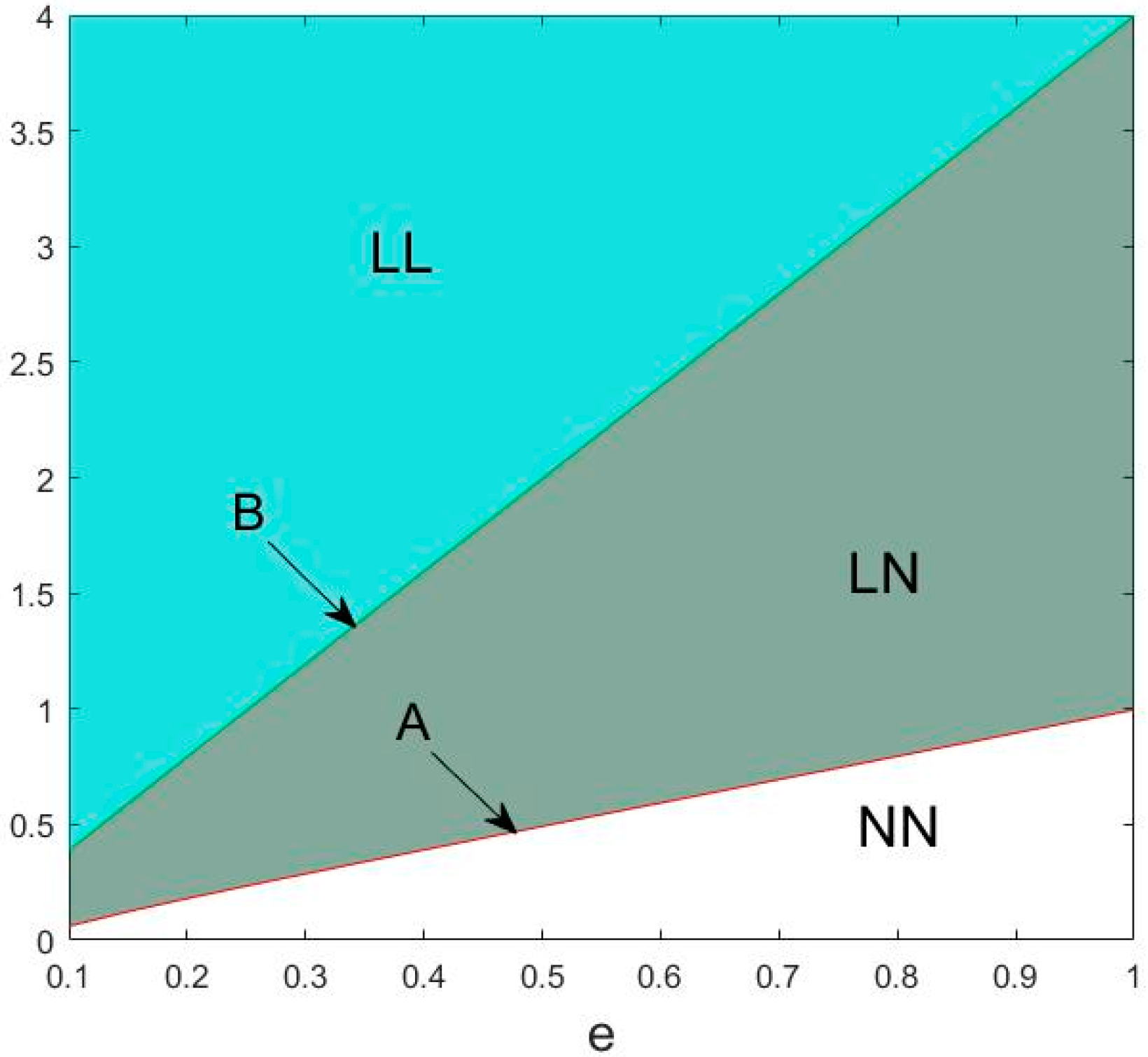
Due to , when , the equilibrium scenario is NN.
Similarly, when , the equilibrium scenario is LN; when , the equilibrium scenario is LL.
However, when , the equilibrium scenario should be NL, although because of , this equilibrium will not exist.
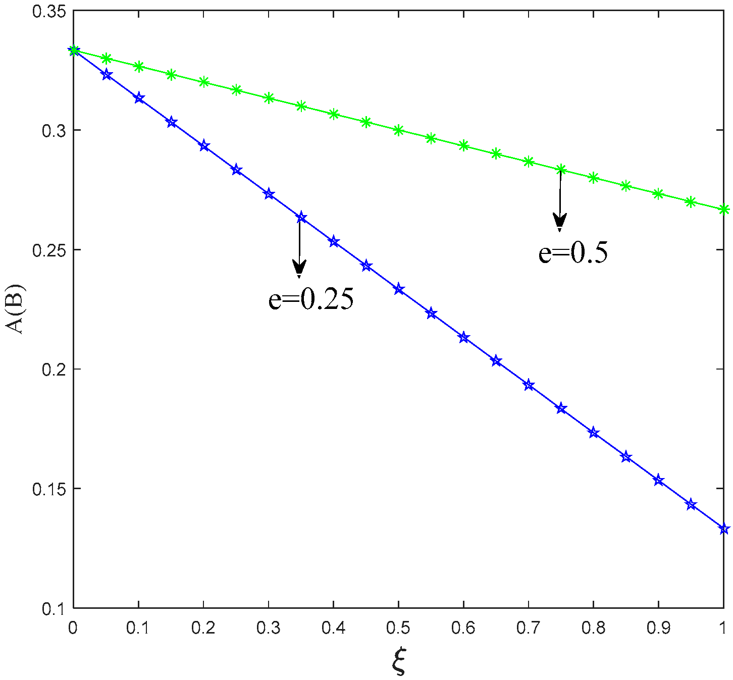
Proof of Lemma 1. .
First, the difference of the demand gap in scenarios LL and NN is determined as follows: .
Given that , , , , , . Thus, .
In the same manner, we can derive . When . In summary, when , .
Similarly, when , we can derive ; when , we can derive .
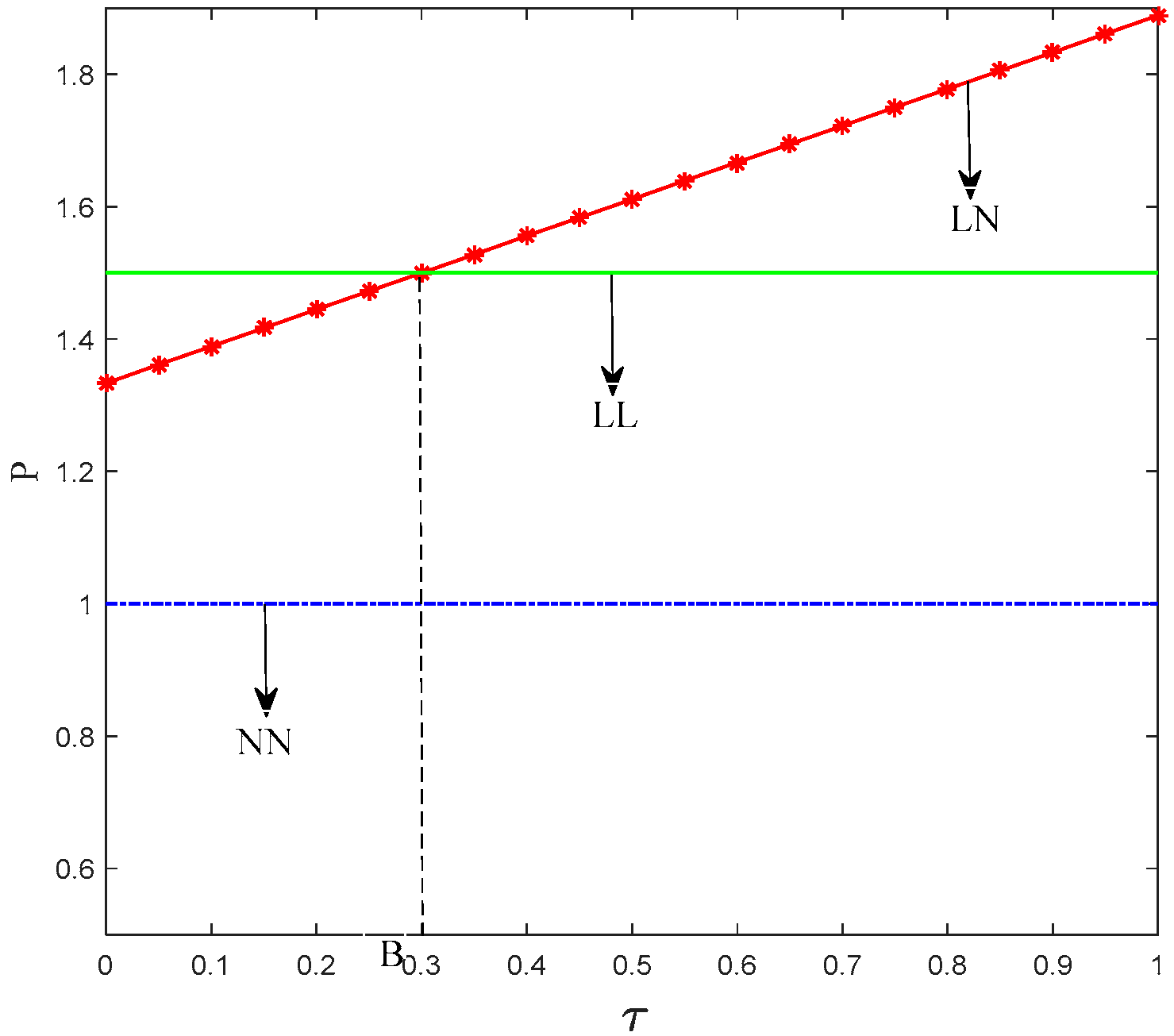
Proof of Proposition 2. Manufacturer 1’s price gap between scenario LN and scenario NN is . Given that , , , , , , we can derive . Thus, is constantly true.
Manufacturer 1’s price gap between scenario LL and scenario NN is . Given that , , , , , we can derive . Thus, is constantly true.
Manufacturer 1’s price gap between scenario LL and scenario LN is . If , , then we can derive ; if , then we can derive .
In summary, if , then ; if , then .
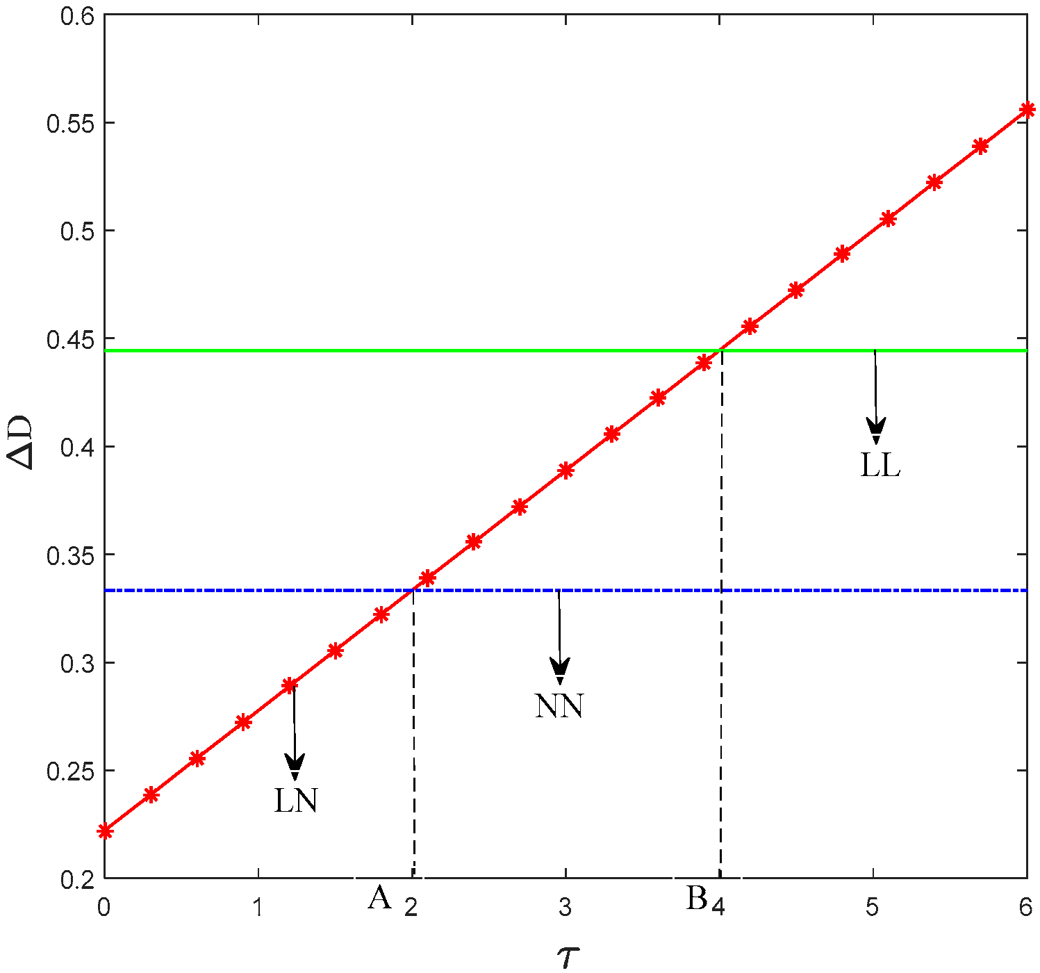
Proof of Lemma 2. Manufacturer 1’s demand gap between scenario LL and scenario NN is . Given that , , and , thus is constantly true.
Manufacturer 1’s demand gap between scenario LL and scenario LN is:
. If , then , and we can derive .
In summary, when , .
Similarly, when , we can derive ; when , we can derive .
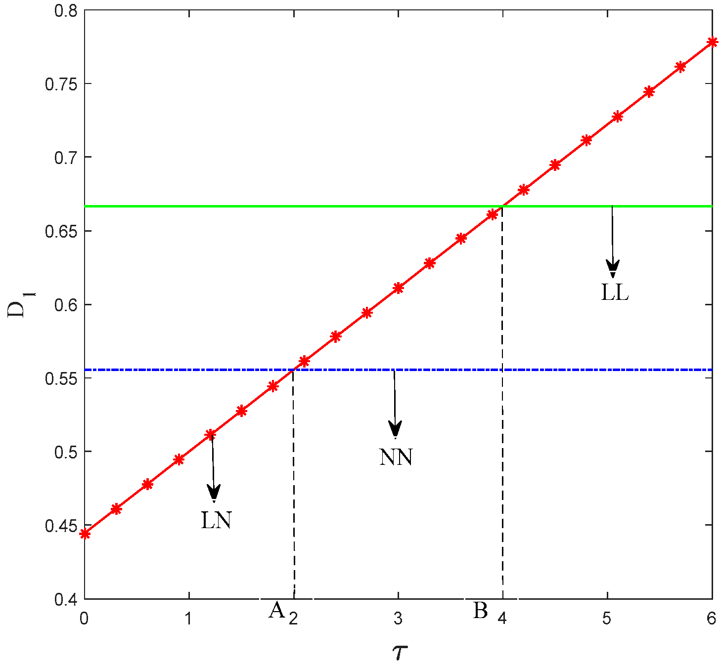
Proof of Lemma 3. , given that , , ; then, .
Similarly, we can prove ,
Proof of Lemma 4. , given that , , , we can derive . Thus, . In the same manner, we can derive and .


