1. Introduction
Cardio-cerebrovascular diseases have become a severe public health issue. In particular, stroke is the primary cause of disability. With the aging population, the ante-displacement of the age of disease onset, and the improvement of the material standard of living, the prevention and treatment of stroke is still a great challenge worldwide [
1,
2]; therefore, the development of new theories and methods is of utmost importance [
3,
4]. Carrying out risk assessments on individuals prior to stroke can provide important information for medical research, hence reduce the social economic burden in the future. To this end, either the effects of multiple covariates for each individual must be determined, or the absolute risk of every person can be calculated through regression or other approaches. The most commonly used regression analysis for risk assessment is the Cox model [
5]. The traditional hazard-based Cox model uses a semi-parametric setting with non-parametric baseline hazard, perfect link and exponential functions. However, although it has been widely used in medical studies, cox model ignores the existence of competing risks.
Medical practice produce a large amount of competing risks data, which is especially related to elderly people [
6,
7]. A common type of competing risks data is survival data with multiple causes of death. For example, in a clinical trial that compares different treatment therapies for breast cancer, interest may be focused on death from breast cancer, but a patient may die due to causes other than breast cancer, such as coronary heart disease, hospital infection, or a traffic accident [
8]. The standard methods for analyzing competing risks data include cause-specific hazard functions [
9,
10], subdistribution hazard model [
11], Framingham models [
12,
13,
14] and fine adjustment Framingham models, depending on the population characteristics. However, the application and imitation of Framingham models have caused many problems, such as variables significant in clinical treatment becoming insignificant in models or coefficients being unexplainable [
15,
16,
17,
18]. Therefore, a more adequate modeling approach is needed for the stroke patients in China.
Sometimes, the observed covariates cannot explain the large proportion of variation in time-to-event data from different areas, for instance, the data of multi-center clinical trials or multi-center cohort studies [
19,
20,
21,
22,
23]. China has a vast territory and many ethnic groups. The heterogeneity of the public in different areas caused by climate, economic level, living habits, and many other factors, is enormous. Therefore, the effects of these latent factors should not be ignored when studying the risk factors of diseases and calculating the absolute risk, even though some of these important factors are unavailable in some circumstances. Furthermore, the effect of a specified covariate should be consistent for individuals at different centers, according to the risk assessment in survival analysis. Therefore, in a multi-center competing risks scenario, with the presence of heterogeneity caused by some latent factors, it is inappropriate to establish different models for every center, even the sample size at each center is sufficient.
In this paper, we demonstrate that most of the predictors (covariates) are not effected by spatial heterogeneity. For example, for smokers with the same amount of cigarette consumption each day, smoking should have the same effect in different areas. That is, the effect of smoke is not related to the smoker’s geographical location. However, it is not ideal if we established different models for different areas, because we may obtain different odds ratios about smoke. Therefore, for multi-center cohort data or multi-center randomized controlled trials (RCT), we established a uniform model for different areas based on the Frailty model [
24,
25,
26,
27], while also setting a center parameter to eliminate the problem detailed above. All the effects of latent factors were incorporated in the center parameter, which was helpful for obtaining accurate and consistent estimators of all of the predictors. Furthermore, based on the Gail model [
28], we estimated the absolute risk of stroke for each person under the competing risks frame. These methods can be easily applied to other cardio-cerebrovascular diseases, and perhaps even to other diseases.
The rest of this paper is organized as follows.
Section 2 reviews the cause-specific hazard model (CSHM), and then introduces the multi-center competing risks model (MCCRM) and the approach of calculating absolute risks.
Section 3 presents the results of the simulation study, assesses the performance of the proposed model, and describes the calibration of the approach to calculate absolute risks.
Section 4 compares the performance of the two models (CSHM and MCCRM) on a dataset from the Shandong Center for Disease Control and Prevention.
Section 5 presents the discussion. Concluding remarks are given in
Section 6.
3. Simulations
In this section, we show the performances of the CSHM and the MCCRM. First, we generated random data with the method introduced by Jan Beyersmann et al. [
7,
29] and then established the two models with random data. Next, we assessed the above-mentioned models through statistical parameters such as bias, standard deviation (SD), root mean square error (RMSE), and area under the curve (AUC). Finally, we calibrated the multi-center competing risks model (MCCRM) by calculating the ratio of the expected number (E) of strokes in the given time interval and compared it with the corresponding observed number (O), i.e., E/O.
In the simulation, we chose stroke as the dependent variable. Death from stroke was the outcome of interest, and death from other causes was the competing risk. Using the Framingham models [
12,
13,
15,
30], we chose five factors as covariates: Total cholesterol (TC), high density lipoprotein (HDL), systolic blood pressure (SBP), diabetes, and smoking. Age and gender were used as stratified variables.
3.1. The Generation of the Dataset
Firstly, we generated the random data of covariates according to the real data used in the study by Zhenxin Zhu et al. [
31]. The real data came from a cohort of all participants who received routine health check-ups from 2005 to 2010 at the Center for Health Management of Shandong Provincial QianFoShan Hospital and the Health Examination Center of Shandong Provincial Hospital. For TC, HDL and SBP were continuous variables, and we calculated the mean vector and covariance matrix of the three covariates using the real data. Then, random data were generated with a multivariate normal distribution. Diabetes and smoke were variables with values of 0–1, which were generated by binomial distribution with the rate of real data from Shouguang City, Shandong Province, China. The center parameter was calculated using Equation (10).
Secondly, due to the existence of competing risks, we generated random data from the dependent variables, which were survival time and survival outcome. As we stratified the data by age and gender, the baseline hazards in Equation (6) could be set as constants, and the covariates could be treated as approximately time-independent; therefore, the distribution of survival time could be simplified as an exponential distribution for each person. The true values of coefficients of the selected five covariates (exposure factors) in Equation (6) were set as according to a rough estimate by the Cox model with real data. As the influence of covariates for other competing risks is always regarded as insignificant, the true values of coefficients of covariates for competing risks in Equation (6) were set as .
At this point, we had obtained the survival time T. Next, we generated the survival outcome X. There were three outcomes, which were indicated by 0, 1, and 2, where 0 referred to a censored outcome, 1 indicated death from stroke, and 2 indicated death from causes other than stroke. We used as the parameter of binomial distribution to generate the outcome (1 or 2) for each sample. We generated random data C with a uniform distribution [0, b], and then specified 0 for the sample if C was smaller than T for each person, or 1 otherwise. The right endpoint b was used to control the censored ratio.
3.2. The Assessment of Models
Then, we were able to establish the CSHM and the MCCRM with the random data generated above. We used the packages survival, pROC, and MASS in R software [
32] to conduct the analysis [
33,
34,
35,
36]. The total sample sizes of the simulated data were N = 1000 and 5000, with censored ratios of Q = 0.2 and 0.4. For each combination of N and Q, we set the standard deviation of the center parameter SDCP to 0.01, 0.05, 0.1, 0.5, 1.0, 1.5, and 2.0, respectively. The cycle time was specified as 1000 for every combination of N, Q, and SDCP. Then, we calculated the means of the bias, SD, RMSE, and AUC. Here, we give three examples (
Table 1,
Table 2 and
Table 3) of combinations of N, Q, and SDCP. The parameter vectors of the N, Q, and SDCP are 5000, 0.2, and 0.01, respectively, for the values given in
Table 1; 5000, 0.2, and 1.0 for the values given in
Table 2; and 5000, 0.2, and 2.0 for the values given in
Table 3.
Table 1 shows that there was no significant difference between the performance of the MCCRM and the CSHM when the SDCP was equal to 0.01. However, when the SDCP was equal to 1.0 or 2.0, the estimate of coefficients of the MCCRM were more precise than those of the CSHM (
Table 2 and
Table 3). Additionally, the AUC of the MCCRM was significantly greater than that of the CSHM. According to the simulation results, the estimators of coefficients of MCCRM can be seen as unbiased compared with the true value
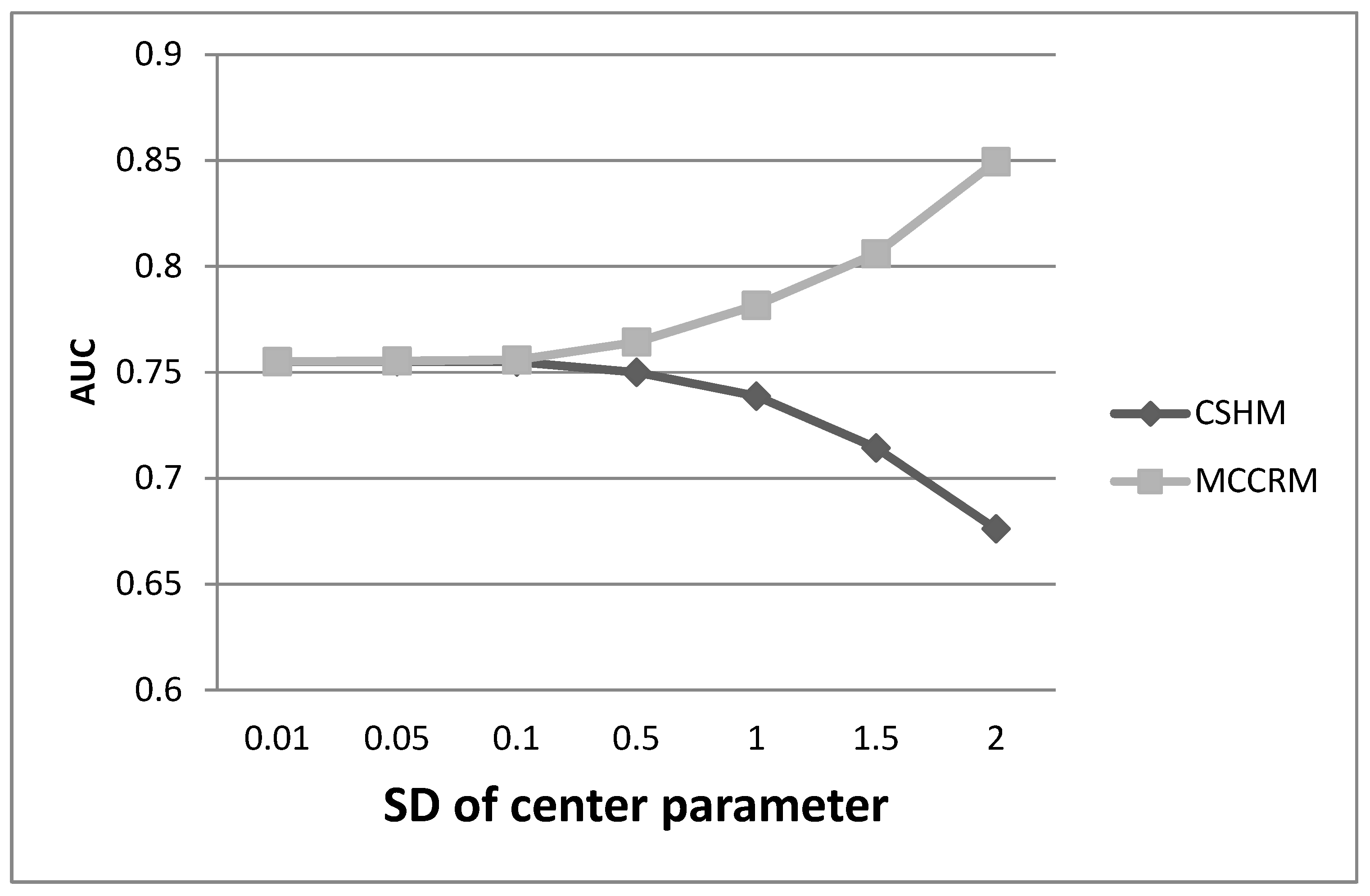
. Furthermore, through a large number of simulations, we found that when the SDCP was less than 0.1, there was no significant difference between the two models. When the SDCP was greater than 0.1, the AUC of the MCCRM was significantly greater than that of the CSHM, and the difference increased progressively with the increase in the SDCP (
Figure 1). When the SDCP was greater than 0.1, the estimate of coefficients of the MCCRM was more precise than those of the CSHM, and the difference was highly significant.
No obvious difference in performance was shown between censor ratios of Q = 0.4 and Q = 0.2. Further the performance was similar with sample sizes of N = 1000 and N = 5000. The robustness of the estimators (bias, SD, RMSE, AUC, E/O, etc.) was not good when N was less than 1000, and the performance of the statistics was robust when N was sufficient.
3.3. The Calibration of Models
Table 4 presents the calibration of the MCCRM. The field name t-
expresses the time interval
SDCP is the standard deviation of the center parameter, and only the simulation results of SDCPs equal to 0.5 or 1.0 are listed. The value of the first cell, 1.0510, represents the E/O at the given time interval [0,1]. E is the expected number, which is the sum of the absolute risk of every sample generated in
Section 3.1. O is the observed number, which is the number of samples whose observed time was less than or equal to 1, and the observed cause was 1 (the outcome of interest).
Table 4 shows that the E/O was acceptable when the SDCP was equal to 0.5. However, when the SDCP was equal to 1.0 and the time length was greater than 3, the E/O was unsatisfactory. Through many simulations, we found that the E/O was acceptable when the SDCP was less than or equal to 0.5 and the time length was less than or equal to 5. Additionally, the precision of E/O decreased linearly with an increase in SDCP.
4. Illustration
We obtained data from the Shandong Center for Disease Control and Prevention study from patients with four diseases (stroke, coronary heart disease (CHD), lung cancer, and stomach cancer) from 17 cities in Shandong Province, China in 2015. For every disease, we had data on the incidence number and population size of the 17 cities, which were stratified by age (five years for each interval). Furthermore, lung cancer and stomach cancer were stratified by gender. We calculated the incidence for each city and then calculated the SDCP after the transformation of incidence using Equation (10).
Table 5 shows SDCP for the four diseases of patients whose age was equal or greater than 40. According to the results in
Section 3, when the SDCP is greater than 0.1, the heterogeneity across different centers cannot be ignored. From
Table 5, we can see that all of the numbers were significantly greater than 0.1; thus, it is necessary to emphasize the importance of the MCCRM during the practical application of multi-center data.
We chose stroke to illustrate the performance of the MCCRM. The results of other diseases were analogous.
Table 6 presents the comparisons of the regression coefficients and the AUC of the two models with stroke. We used the stroke incidence of the 17 cities to generate the center parameter with Equation (10), and the age interval was equal or greater than 50 and less than 55. The covariates survival time and survival outcome were generated by the same method introduced in detail in
Section 3. The sample size was 5000, and the censored ratio was 0.2. The SDCP 1.047 of ages 50 to 55, which according to
Table 5, is obviously greater than 0.1.
As the results of the simulation in
Section 3,
Table 6 shows that all of the estimators (bias, SD, RMSE) of the MCCRM were more precise and superior to the corresponding estimators of the CSHM. For example, the maximum of RMSE of the CSHM was 0.8580, while the RMSE of the same covariate (HDL) in the MCCRM was 0. 079. The AUC of the MCCRM was 0.7994, while the AUC of the CSHM was only 0.7205.
5. Discussion
A common question arising in multi-center random clinical trials and multi-center cohort studies where competing risks exist is whether any heterogeneity in outcomes exists, and whether the heterogeneity has an obvious influence on the research target. Therefore, it is necessary to choose the appropriate model and determine whether statistical adjustment is required while estimating the effect of risk factors or calculating the absolute risk of a certain disease. When analyzing multi-center survival data, frailty survival models have been shown being useful, notably with regard to the usual large number of centers and low number of patients in each center [
37,
38]. Nevertheless, frailty survival models do not provide any detailed differences of the CSHM and frailty models. Through the simulation in
Section 3, we have provided a precise analysis of the CSHM and the MCCRM by changing the sample size, censored ratio, the standard deviation of the center parameter, and the number of centers, among other factors. Theoretical studies will be presented in follow-up work.
With existing competing risks, Bayesian statistics have been reported to be more useful and efficient for assessing prior information, variable selection, and absolute risk [
39,
40,
41,
42]. Moreover, Bayesian models are more flexible than empirical models. However, in this paper, in order to emphasize the importance of heterogeneity, we have only mentioned the multi-center data, and did not take prior information into account. The limitation of this paper is that only baseline data are used for prediction, and the situation of multiple follow-up observations is not fully considered. This will inevitably affect the accuracy of predicting absolute risk and the stability of the model. In our follow-up work, we will consider combining the multiple follow-up observations, the prior information and multi-center data under a competing risks scenario.
6. Conclusions
Through Equation (10), we calculated the SDCP, which helped us select the most appropriate model according to the physical truth. When the SDCP was less than 0.1, the MCCRM and CSHM performed analogously, so either could be selected randomly for the practical application. When the SDCP was equal to or greater than 0.1, the performance of the MCCRM was significantly superior to the CSHM according to estimators such as bias, SD, RMSE, AUC, and E/O. Furthermore, when the SDCP was too big, the CSHM became inefficient, then the MCCRM should be selected as the appropriate model. Therefore, MCCRM can help us make full use of multi-center data and give accurate estimates of covariate coefficients. Moreover, the covariate coefficients of the MCCRM are consistent for different centers or areas, so the explanation of covariate coefficients has become more simple and reasonable.
Using Equation (11) and the MCCRM, the absolute risk of stroke occurring for a certain person was calculated. The approach of calculating absolute risk was excellent when the time interval was not too large, according to the calibration in
Section 3. That is, short time intervals were predicted more precisely than long time intervals. However, only having the baseline value of covariates in a cohort study may cause inaccuracy in long time interval prediction.


