Physician Behavior under Prospective Payment Schemes—Evidence from Artefactual Field and Lab Experiments


Abstract
:1. Introduction
2. Experimental Design
2.1. Framing and Subject Pool
2.2. Group Composition and Roles
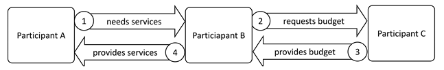
2.3. Relationship between the Group Members
2.4. Roles and Payoffs
2.4.1. Patient
2.4.2. Physician
2.4.3. Insurer
2.5. Physician Decision Problem and Conjectures
2.6. Experimental Protocol
3. Results
3.1. Average Provision Behavior
3.2. Differences between Fee For Service and Capitation
3.3. Differences between Neutral and Medical Framing
3.4. Differences between Student and Physician Samples
3.5. Regression Analysis—Payoffs and Experimental Variations
4. Discussion and Conclusions
Author Contributions
Funding
Acknowledgments
Conflicts of Interest
Appendix A. Reporting Behavior
Appendix A.1. Differences in Reporting between Fee for Service and Capitation


| Payment System | ||||
|---|---|---|---|---|
| Patient | Fram.-Subj. | FFS | CAP | U-Test |
| Neutr.-Stud. | 1 | 0.22 | *** | |
| L | Med.-Stud. | 0.44 | 0.13 | * |
| Med.-Doc. | 0 | 0 | ||
| Neutr.-Stud. | 0.56 | 0.04 | *** | |
| M | Med.-Stud. | 0.52 | 0.33 | |
| Med.-Doc. | 0.33 | 0.08 | ||
| Neutr.-Stud. | 0 | −0.15 | * | |
| H | Med.-Stud. | −0.04 | −0.04 | |
| Med.-Doc. | 0 | −0.08 | ||
Appendix A.2. Differences in Reporting between Neutral and Medical Framing
| Framing | ||||
|---|---|---|---|---|
| Patient | Payment System | Neutral | Medical | U-Test |
| L | FFS | 1 | 0.44 | ** |
| CAP | 0.22 | 0.13 | ||
| M | FFS | 0.56 | 0.52 | |
| CAP | 0.04 | 0.33 | ** | |
| H | FFS | 0 | −0.04 | |
| CAP | −0.15 | −0.04 | ||
Appendix A.3. Differences in Reporting between Student and Physician Samples
| Subjects | ||||
|---|---|---|---|---|
| Patient | Payment System | Students | Doctors | U-Test |
| L | FFS | 0.44 | 0 | * |
| CAP | 0.13 | 0 | ||
| M | FFS | 0.52 | 0.33 | |
| CAP | 0.33 | 0.08 | ||
| H | FFS | −0.04 | 0 | |
| CAP | −0.04 | −0.08 | ||
Appendix A.4. Provision Conditional on Reporting
Appendix B. Additional Tables
| Treatment | Avg. Misreporting | Treatment | CNS | CMS | CMD | FNS | FMS | |
|---|---|---|---|---|---|---|---|---|
| CNS | 0.22 ** | CNS | ||||||
| CMS | 0.13 * | CMS | ||||||
| CMD | 0 | CMD | ||||||
| FNS | 1 *** | FNS | *** | *** | *** | |||
| FMS | 0.44 *** | FMS | * | * | ** | |||
| FMD | 0 | FMD | *** | * |
| Treatment | Avg. Misreporting | Treatment | CNS | CMS | CMD | FNS | FMS | |
|---|---|---|---|---|---|---|---|---|
| CNS | 0.04 | CNS | ||||||
| CMS | 0.33 *** | CMS | ** | |||||
| CMD | 0.08 | CMD | ||||||
| FNS | 0.56 *** | FNS | *** | *** | ||||
| FMS | 0.52 *** | FMS | *** | ** | ||||
| FMD | 0.33 ** | FMD | * |
| Treatment | Avg. Misreporting | Treatment | CNS | CMS | CMD | FNS | FMS | |
|---|---|---|---|---|---|---|---|---|
| CNS | −0.15 * | CNS | ||||||
| CMS | −0.04 | CMS | ||||||
| CMD | −0.08 | CMD | ||||||
| FNS | 0 | FNS | * | |||||
| FMS | −0.04 | FMS | ||||||
| FMD | 0 | FMD |
| Treatment | Avg. Misreporting | Treatment | CNS | CMS | CMD | FNS | FMS | |
|---|---|---|---|---|---|---|---|---|
| CNS | 0.04 | CNS | ||||||
| CMS | 0.08 | CMS | ||||||
| CMD | 0 | CMD | ||||||
| FNS | 2.11 *** | FNS | *** | *** | *** | |||
| FMS | 0.96 *** | FMS | *** | *** | *** | ** | ||
| FMD | 0 | FMD | *** | ** |
| Treatment | Avg. Maltreatment | Treatment | CNS | CMS | CMD | FNS | FMS | |
|---|---|---|---|---|---|---|---|---|
| CNS | −1 *** | CNS | ||||||
| CMS | −0.83 *** | CMS | ||||||
| CMD | −1.08 *** | CMD | ||||||
| FNS | 0.44 * | FNS | *** | *** | *** | |||
| FMS | −0.04 | FMS | *** | ** | ** | |||
| FMD | −0.89 *** | FMD | ** |
| Treatment | Avg. Maltreatment Treatment | CNS | CMS | CMD | FNS | FMS | ||
|---|---|---|---|---|---|---|---|---|
| CNS | −0.63 *** | CNS | ||||||
| CMS | −0.54 ** | CMS | ||||||
| CMD | −0.75 * | CMD | ||||||
| FNS | −0.26 * | FNS | ** | |||||
| FMS | −0.33 ** | FMS | ||||||
| FMD | 0 | FMD | * |
| Treatment | Avg. Maltreatment | Treatment | CNS | CMS | CMD | FNS | FMS | |
|---|---|---|---|---|---|---|---|---|
| CNS | 0.11 ** | CNS | ||||||
| CMS | 0.33 *** | CMS | * | |||||
| CMD | 0.08 | CMD | ||||||
| FNS | 0.63 *** | FNS | *** | ** | *** | |||
| FMS | 0.52 *** | FMS | *** | ** | ||||
| FMD | 0.33 ** | FMD |
| Treatment | Avg. Maltreatment | Treatment | CNS | CMS | CMD | FNS | FMS | |
|---|---|---|---|---|---|---|---|---|
| CNS | 1 *** | CNS | ||||||
| CMS | 0.83 *** | CMS | ||||||
| CMD | 1.08 *** | CMD | ||||||
| FNS | 1.41 *** | FNS | *** | *** | ||||
| FMS | 1.15 *** | FMS | * | |||||
| FMD | 0.89 *** | FMD | * |
| Treatment | Reported Type | Provided Services | ||||||
|---|---|---|---|---|---|---|---|---|
| 1 | 2 | 3 | 4 | 5 | 6 | Obs. | ||
| L | 0 | 23 | 0 | 23 | ||||
| CNS | M | 0 | 1 | 1 | 2 | |||
| H | 1 | 0 | 1 | 0 | 0 | 0 | 2 | |
| L | 0 | 22 | 0 | 22 | ||||
| CMS | M | 0 | 1 | 0 | 1 | |||
| H | 0 | 0 | 0 | 1 | 0 | 0 | 1 | |
| L | 0 | 12 | 0 | 12 | ||||
| CMD | M | 0 | 0 | 0 | 0 | |||
| H | 0 | 0 | 0 | 0 | 0 | 0 | 0 | |
| 1 | 2 | 3 | 4 | 5 | 6 | Obs. | ||
| L | 1 | 4 | 8 | 13 | ||||
| FNS | M | 0 | 0 | 1 | 1 | |||
| H | 0 | 0 | 1 | 0 | 0 | 12 | 13 | |
| L | 2 | 8 | 10 | 20 | ||||
| FMS | M | 0 | 0 | 2 | 2 | |||
| H | 0 | 1 | 0 | 0 | 0 | 4 | 5 | |
| L | 0 | 9 | 0 | 9 | ||||
| FMD | M | 0 | 0 | 0 | 0 | |||
| H | 0 | 0 | 0 | 0 | 0 | 0 | 0 | |
| Treatment | Reported Type | Provided Services | ||||||
|---|---|---|---|---|---|---|---|---|
| 1 | 2 | 3 | 4 | 5 | 6 | Obs. | ||
| L | 0 | 0 | 1 | 1 | ||||
| CNS | M | 0 | 1 | 23 | 24 | |||
| H | 0 | 0 | 1 | 1 | 0 | 0 | 2 | |
| L | 0 | 0 | 0 | 0 | ||||
| CMS | M | 0 | 0 | 16 | 16 | |||
| H | 0 | 2 | 0 | 6 | 0 | 0 | 8 | |
| L | 0 | 0 | 0 | 0 | ||||
| CMD | M | 0 | 2 | 9 | 11 | |||
| H | 0 | 0 | 0 | 1 | 0 | 0 | 1 | |
| L | 1 | 0 | 0 | 1 | ||||
| FNS | M | 0 | 0 | 10 | 10 | |||
| H | 0 | 0 | 0 | 2 | 3 | 11 | 16 | |
| L | 0 | 0 | 0 | 0 | ||||
| FMS | M | 0 | 2 | 11 | 13 | |||
| H | 0 | 0 | 1 | 3 | 5 | 5 | 14 | |
| L | 0 | 0 | 0 | 0 | ||||
| FMD | M | 0 | 1 | 5 | 6 | |||
| H | 0 | 0 | 1 | 2 | 0 | 0 | 3 | |
| Treatment | Reported Type | Provided Services | ||||||
|---|---|---|---|---|---|---|---|---|
| 1 | 2 | 3 | 4 | 5 | 6 | Obs. | ||
| L | 1 | 0 | 0 | 1 | ||||
| CNS | M | 0 | 0 | 2 | 2 | |||
| H | 0 | 0 | 0 | 1 | 4 | 19 | 24 | |
| L | 0 | 0 | 0 | 0 | ||||
| CMS | M | 0 | 0 | 1 | 1 | |||
| H | 1 | 0 | 1 | 1 | 0 | 20 | 23 | |
| L | 0 | 0 | 0 | 0 | ||||
| CMD | M | 1 | 0 | 0 | 1 | |||
| H | 0 | 0 | 1 | 0 | 1 | 9 | 11 | |
| L | 0 | 0 | 0 | 0 | ||||
| FNS | M | 0 | 0 | 0 | 0 | |||
| H | 1 | 0 | 0 | 1 | 0 | 25 | 27 | |
| 1 | 2 | 3 | 4 | 5 | 6 | Obs. | ||
| L | 0 | 0 | 0 | 0 | ||||
| FMS | M | 0 | 1 | 0 | 1 | |||
| H | 0 | 0 | 0 | 1 | 3 | 22 | 26 | |
| L | 0 | 0 | 0 | 0 | ||||
| FMD | M | 0 | 0 | 0 | 0 | |||
| H | 0 | 0 | 0 | 0 | 0 | 9 | 9 | |
| Patient | Physician | Insurer | |||||||
|---|---|---|---|---|---|---|---|---|---|
| Patient Type L | Fee For Service | −28.57 *** | −29.06 *** | −0.51 | −0.46 | −10.51 *** | −10.91 *** | ||
| (3.82) | (3.83) | (2.97) | (2.96) | (2.72) | (2.72) | ||||
| Medical Framing | 11.02 *** | 10.75 ** | −8.76 *** | −9.29 *** | 7.52 ** | 7.28 ** | |||
| (4.18) | (4.31) | (3.25) | (3.33) | (2.97) | (3.06) | ||||
| Medical Doctor | 11.94 ** | 9.50 | −5.68 | −4.35 | 4.23 | 6.18 | |||
| (5.56) | (9.26) | (4.32) | (7.15) | (3.96) | (6.57) | ||||
| Age | - | 0.25 | - | −0.16 | - | −0.08 | |||
| - | (0.52) | - | (0.40) | - | (0.37) | ||||
| Female | - | 6.92 | - | −7.04 ** | - | 4.73 | |||
| - | (4.27) | - | (3.29) | - | (3.03) | ||||
| Pro Social | - | −4.24 | - | 1.75 | - | −4.11 | |||
| - | (4.02) | - | (3.10) | - | (2.85) | ||||
| Risk | - | 0.43 | - | −0.24 | - | 0.41 | |||
| - | (0.89) | - | (0.69) | - | (0.63) | ||||
| Constant | 74.79 *** | 64.98 *** | 56.09 *** | 64.59 *** | 77.76 *** | 76.79 *** | |||
| (3.48) | (12.90) | (2.70) | (9.96) | (2.48) | (9.15) | ||||
| Patient Type M | Fee For Service | −7.32 *** | −7.55 *** | 10.46 *** | 11.12 *** | −15.27 *** | −15.80 *** | ||
| (2.66) | (2.60) | (2.56) | (2.51) | (3.52) | (3.50) | ||||
| Medical Framing | 5.72 ** | 5.83 ** | −3.64 | −2.90 | −3.96 | −4.72 | |||
| (2.91) | (2.93) | (2.80) | (2.82) | (3.85) | (3.94) | ||||
| Medical Doctor | −0.74 | 11.15 * | −5.37 | 5.36 | 9.30 * | −4.33 | |||
| (3.88) | (6.29) | (3.73) | (6.06) | (5.12) | (8.47) | ||||
| Age | - | −0.77 ** | - | −0.81 ** | - | 0.99 ** | |||
| - | (0.35) | - | (0.34) | - | (0.47) | ||||
| Female | - | 3.98 | - | −5.30 * | - | 3.76 | |||
| - | (2.90) | - | (2.79) | - | (3.90) | ||||
| Pro Social | - | −5.29 * | - | 2.43 | - | −0.96 | |||
| - | (2.73) | - | (2.63) | - | (3.67) | ||||
| Risk | - | 0.49 | - | −0.40 | - | 0.12 | |||
| - | (0.60) | - | (0.58) | - | (0.81) | ||||
| Constant | 56.66 *** | 72.18 *** | 53.10 *** | 75.29 *** | 77.64 *** | 52.82 *** | |||
| (2.43) | (8.77) | (2.33) | (8.44) | (3.21) | (11.80) | ||||
| Patient Type H | Fee For Service | 8.66 ** | 6.84 * | 36.30 *** | 36.03 *** | −2.85 * | −2.71 | ||
| (4.16) | (4.09) | (1.65) | (1.65) | (1.69) | (1.71) | ||||
| Medical Framing | −0.31 | −3.97 | −0.59 | −1.05 | −0.65 | −0.14 | |||
| (4.55) | (4.61) | (1.80) | (1.86) | (1.85) | (1.92) | ||||
| Medical Doctor | 1.93 | 2.06 | 2.27 | 5.91 | 0.09 | 3.95 | |||
| (6.06) | (9.88) | (2.40) | (3.99) | (2.46) | (4.13) | ||||
| Age | - | 0.02 | - | −0.25 | - | −0.26 | |||
| - | (0.55) | - | (0.22) | - | (0.23) | ||||
| Female | - | −3.21 | - | −0.90 | - | 0.93 | |||
| - | (4.55) | - | (1.84) | - | (1.90) | ||||
| Pro Social | - | −11.80 *** | - | −2.07 | - | 0.48 | |||
| - | (4.29) | - | (1.73) | - | (1.79) | ||||
| Risk | - | 0.60 | - | 0.22 | - | 0.17 | |||
| - | (0.95) | - | (0.38) | - | (0.40) | ||||
| Constant | 71.17 *** | 77.16 *** | 49.91 *** | 56.37 *** | 43.93 *** | 48.13 *** | |||
| (3.79) | (13.77) | (1.50) | (5.57) | (1.54) | (5.75) | ||||
Appendix C. Instructions Neutral Framing
General Information
The Experiment
| Type | Optimal number of services |
| L | 2 units |
| M | 4 units |
| H | 6 units |
- If the number of services provided by participant B is optimal for participant A, he/she receives a payment of 90 Taler with a probability of 95%. With a probability of 5% she receives a payment of 0 Taler.
- If the number of actually provided services by participant B deviates by one unit from the optimal number of services for participant A, participant A receives a payment of 90 Taler with a probability of 65%. With a probability of 35% he/she receives a payment of 0 Taler.
- If the number of actually provided services by participant B deviates by two units from the optimal number of services for participant A, participant A receives a payment of 90 Taler with a probability of 35%. With a probability of 65% he/she receives a payment of 0 Taler.
- If the number of actually provided services by participant B deviates by three units or more from the optimal number of services for participant A, participant A receives a payment of 90 Taler with a probability of 5%. With a probability of 95% he/she receives a payment of 0 Taler.
| Participant A of type L | ||
| Number of services provided | Probability for | Probability for |
| by participant B | payment of 90 | payment of 0 |
| 1 | 65% | 35% |
| 2 | 95% | 5% |
| 3 | 65% | 35% |
| 4 | 35% | 65% |
| 5 | 5% | 95% |
| 6 | 5% | 95% |
| Participant A of type M | ||
| Number of services provided | Probability for | Probability for |
| by participant B | payment of 90 | payment of 0 |
| 1 | 5% | 95% |
| 2 | 35% | 65% |
| 3 | 65% | 35% |
| 4 | 95% | 5% |
| 5 | 65% | 35% |
| 6 | 35% | 65% |
| Participant A of type H | ||
| Number of services provided | Probability for | Probability for |
| by participant B | payment of 90 | payment of 0 |
| 1 | 5% | 95% |
| 2 | 5% | 95% |
| 3 | 5% | 95% |
| 4 | 35% | 35% |
| 5 | 65% | 65% |
| 6 | 95% | 5% |
| Budget Group | Cost Table | ||||
| Type | Budged Group | Budget | Service Units | Total Costs | |
| L | I | 45 | 1 | 15 | |
| 2 | 30 | ||||
| M | 3 | 45 | |||
| H | II | 90 | 4 | 60 | |
| 5 | 75 | ||||
| 6 | 90 | ||||
- (1)
- Participant B learns in every situation which of the three possible types participant A is in the current case. Participant A and participant C do not have any information about the type of participant A at any point of time.
- (2)
- Participant B tells participant C which type participant A is.
- (3)
- On the basis of his/her message about participant A, participant B will be provided a budget group. The budget associated with that will be subtracted from the endowment of participant C.
- (4)
- Participant B decides which number of services she wants to provide for participant A.
Appendix D. Instructions Medical Framing
General Information
The Experiment
| Type | Optimal number of Medical Services |
| L | 2 units |
| M | 4 units |
| H | 6 units |
- If the number of Medical Services provided by the Physician is optimal for the Patient, he/she receives a payment of 90 Taler with a probability of 95%. With a probability of 5% she receives a payment of 0 Taler.
- If the number of actually provided Medical Services by the Physician deviates by one unit from the optimal number of Medical Services for the Patient, the Patient receives a payment of 90 Taler with a probability of 65%. With a probability of 35% he/she receives a payment of 0 Taler.
- If the number of actually provided Medical Services by the Physician deviates by two units from the optimal number of Medical Services for the Patient, the Patient receives a payment of 90 Taler with a probability of 35%. With a probability of 65% he/she receives a payment of 0 Taler.
- If the number of actually provided Medical Services by the Physician deviates by three units or more from the optimal number of Medical Services for the Patient, the Patient receives a payment of 90 Taler with a probability of 5%. With a probability of 95% he/she receives a payment of 0 Taler.
| Patient of type L | ||
| Number of Medical Services provided | Probability for | Probability for |
| by participant B | payment of 90 | payment of 0 |
| 1 | 65% | 35% |
| 2 | 95% | 5% |
| 3 | 65% | 35% |
| 4 | 35% | 65% |
| 5 | 5% | 95% |
| 6 | 5% | 95% |
| Patient of type M | ||
| Number of Medical Services provided | Probability for | Probability for |
| by participant B | payment of 90 | payment of 0 |
| 1 | 5% | 95% |
| 2 | 35% | 65% |
| 3 | 65% | 35% |
| 4 | 95% | 5% |
| 5 | 65% | 35% |
| 6 | 35% | 65% |
| Patient of type H | ||
| Number of Medical Services provided | Probability for | Probability for |
| by participant B | payment of 90 | payment of 0 |
| 1 | 5% | 95% |
| 2 | 5% | 95% |
| 3 | 5% | 95% |
| 4 | 35% | 35% |
| 5 | 65% | 65% |
| 6 | 95% | 5% |
| Budget Group | Cost Table | ||||
| Type | Budged Group | Budget | Service Units | Total Costs | |
| L | I | 45 | 1 | 15 | |
| 2 | 30 | ||||
| M | 3 | 45 | |||
| H | II | 90 | 4 | 60 | |
| 5 | 75 | ||||
| 6 | 90 | ||||
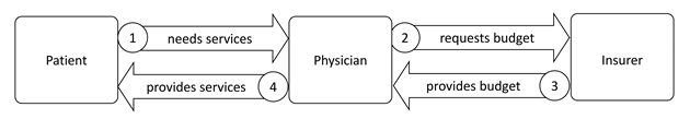
- (1)
- The Physician learns in every situation which of the three possible types the Patient is in the current case. The Patient and the Health Insurance do not have any information about the type of the Patient at any point of time.
- (2)
- The Physician tells the Health Insurance which type the Patient is.
- (3)
- On the basis of her message about the Patient, the Physician will be provided a budget group. The budget associated with that will be subtracted from the endowment of the Health Insurance.
- (4)
- The Physician decides which number of Medical Services she wants to provide for the Patient.
Appendix E. Control Questions Neutral Framing
Appendix F. Control Questions Medical Framing
Appendix G. Screenshots of Experimental Decision


References
- Arrow, K.J. Uncertainty and the welfare economics of medical care. Am. Econ. Rev. 1963, 53, 941–973. [Google Scholar]
- McGuire, T.G. Physician agency. Handb. Health Econ. 2000, 1, 461–536. [Google Scholar]
- Chandra, A.; Cutler, D.; Song, Z. Who ordered that? The economics of treatment choices in medical care. Handb. Health Econ. 2012, 2, 397–432. [Google Scholar]
- Coey, D. Physicians’ financial incentives and treatment choices in heart attack management. Quant. Econ. 2015, 6, 703–748. [Google Scholar] [CrossRef]
- Chalkley, M.; Listl, S. First do no harm—The impact of financial incentives on dental X-rays. J. Health Econ. 2018, 58, 1–9. [Google Scholar] [CrossRef]
- Brekke, K.R.; Holmås, T.H.; Monstad, K.; Straume, O.R. Do treatment decisions depend on physicians’ financial incentives? J. Public Econ. 2017, 155, 74–92. [Google Scholar] [CrossRef] [Green Version]
- Hennig-Schmidt, H.; Selten, R.; Wiesen, D. How payment systems affect physicians’ provision behaviour—An experimental investigation. J. Health Econ. 2011, 30, 637–646. [Google Scholar] [CrossRef] [Green Version]
- Godager, G.; Wiesen, D. Profit or patient’s health benefit? Exploring the heterogeneity in physician altruism. J. Health Econ. 2013, 32, 1105–1116. [Google Scholar] [CrossRef] [Green Version]
- Brosig-Koch, J.; Hennig-Schmidt, H.; Kairies, N.; Wiesen, D. How Effective Are Pay-for-Performance Incentives for Physicians? A Laboratory Experiment; Ruhr Economic Papers 413; Ruhr-Universität Bochum, University of Dortmund: Dortmund, Germany; University of Duisburg-Essen and RWI Essen: Essen, Germany, 2013. [Google Scholar]
- Keser, C.; Montmarquette, C.; Schmidt, M.; Schnitzler, C. Custom-Made Healthcare—An Experimental Investigation; CEGE Discussion Papers No. 218; Georg-August-University Göttingen: Göttingen, Germany, 2014. [Google Scholar]
- Green, E.P. Payment systems in the healthcare industry: An experimental study of physician incentives. J. Econ. Behav. Organ. 2014, 106, 367–378. [Google Scholar] [CrossRef] [Green Version]
- Brosig-Koch, J.; Hennig-Schmidt, H.; Kairies-Schwarz, N.; Kokot, J.; Wiesen, D. Physician Performance Pay: Experimental Evidence. 2019. Available online: https://ssrn.com/abstract=3467583 (accessed on 29 June 2020).
- Brosig-Koch, J.; Hennig-Schmidt, H.; Kairies, N.; Wiesen, D. The Effects of Introducing Mixed Payment Systems for Physicians: Experimental Evidence. Health Econ. 2017, 26, 243–262. [Google Scholar] [CrossRef] [Green Version]
- Di Guida, S.; Gyrd-Hansen, D.; Oxholm, A.S. Testing the myth of fee-for-service and overprovision in health care. Health Econ. 2019, 28, 717–722. [Google Scholar] [CrossRef] [PubMed]
- Chandra, A.; Skinner, J. Technology growth and expenditure growth in health care. J. Econ. Lit. 2012, 50, 645–680. [Google Scholar] [CrossRef] [Green Version]
- Hassell, K.; Atella, V.; Schafheutle, E.I.; Weiss, M.C.; Noyce, P.R. Cost to the patient or cost to the healthcare system? Which one matters the most for GP prescribing decisions? Eur. J. Public Health 2003, 13, 18–23. [Google Scholar] [CrossRef] [PubMed] [Green Version]
- Tilburt, J.C.; Wynia, M.K.; Sheeler, R.D.; Thorsteinsdottir, B.; James, K.M.; Egginton, J.S.; Liebow, M.; Hurst, S.; Danis, M.; Goold, S.D. Views of US physicians about controlling health care costs. JAMA 2013, 310, 380–389. [Google Scholar] [CrossRef] [Green Version]
- Pedersen, L.B.; Riise, J.; Hole, A.R.; Gyrd-Hansen, D. GPs’ shifting agencies in choice of treatment. Appl. Econ. 2014, 46, 750–761. [Google Scholar] [CrossRef]
- Andreoni, J. Giving gifts to groups: How altruism depends on the number of recipients. J. Public Econ. 2007, 91, 1731–1749. [Google Scholar] [CrossRef] [Green Version]
- Schumacher, H.; Kesternich, I.; Kosfeld, M.; Winter, J. One, Two, Many–Insensitivity to Group Size in Games with Concentrated Benefits and Dispersed Costs. Rev. Econ. Stud. 2017, 84, 1346–1377. [Google Scholar] [CrossRef]
- Busse, R.; Geissler, A.; Quentin, W.; Wiley, M. Diagnosis-Related Groups in Europe. Moving towards tRansparency, Efficiency and Quality in Hospitals. 2011. Available online: https://www.euro.who.int/__data/assets/pdf_file/0004/162265/e96538.pdf (accessed on 29 June 2020).
- Davis, C.K.; Rhodes, D.J. The impact of DRGs on the cost and quality of health care in the United States. Health Policy 1988, 9, 117–131. [Google Scholar] [CrossRef]
- Moreno-Serra, R.; Wagstaff, A. System-wide impacts of hospital payment reforms: Evidence from Central and Eastern Europe and Central Asia. J. Health Econ. 2010, 29, 585–602. [Google Scholar] [CrossRef] [Green Version]
- Cutler, D.M. The incidence of adverse medical outcomes under prospective payments. Econometrica 1995, 63, 29–50. [Google Scholar] [CrossRef]
- Dafny, L.S. How Do Hospitals Respond to Price Changes? Am. Econ. Rev. 2005, 95, 1525–1547. [Google Scholar] [CrossRef] [PubMed] [Green Version]
- Silverman, E.; Skinner, J. Medicare upcoding and hospital ownership. J. Health Econ. 2004, 23, 369–389. [Google Scholar] [CrossRef]
- Jürges, H.; Köberlein, J. What explains DRG upcoding in neonatology? The roles of financial incentives and infant health. J. Health Econ. 2015, 43, 13–26. [Google Scholar] [CrossRef] [PubMed]
- Fang, H.; Gong, Q. Detecting Potential Overbilling in Medicare Reimbursement via Hours Worked. Am. Econ. Rev. 2017, 107, 562–591. [Google Scholar] [CrossRef] [PubMed]
- Reif, S.; Wichert, S.; Wuppermann, A. Is it good to be too light? Birth weight thresholds in hospital reimbursement systems. J. Health Econ. 2018, 59, 1–25. [Google Scholar] [CrossRef] [Green Version]
- Hennig-Schmidt, H.; Jürges, H.; Wiesen, D. Dishonesty in health care practice: A behavioral experiment on upcoding in neonatology. Health Econ. 2019, 28, 319–338. [Google Scholar] [CrossRef]
- Charness, G.; Rabin, M. Understanding social preferences with simple tests. Q. J. Econ. 2002, 117, 817–869. [Google Scholar] [CrossRef] [Green Version]
- Engelmann, D.; Strobel, M. Inequality aversion, efficiency, and maximin preferences in simple distribution experiments. Am. Econ. Rev. 2004, 94, 857–869. [Google Scholar] [CrossRef] [Green Version]
- Engel, C. Dictator games: A meta study. Exp. Econ. 2011, 14, 583–610. [Google Scholar] [CrossRef]
- Lagarde, M.; Blaauw, D. Physicians’ responses to financial and social incentives: A medically framed real effort experiment. Soc. Sci. Med. 2017, 179, 147–159. [Google Scholar] [CrossRef] [Green Version]
- Brosig-Koch, J.; Hennig-Schmidt, H.; Kairies-Schwarz, N.; Wiesen, D. Using artefactual field and lab experiments to investigate how fee-for-service and capitation affect medical service provision. J. Econ. Behav. Organ. 2016, 131, 17–23. [Google Scholar] [CrossRef] [Green Version]
- Kairies, N.; Krieger, M. How do Non-Monetary Performance Incentives for Physicians Affect the Quality of Medical Care?—A Laboratory Experiment; Ruhr Economic Papers 414; Ruhr-Universität Bochum, University of Dortmund: Dortmund, Germany; University of Duisburg-Essen and RWI Essen: Essen, Germany, 2013. [Google Scholar]
- Abbink, K.; Hennig-Schmidt, H. Neutral versus loaded instructions in a bribery experiment. Exp. Econ. 2006, 9, 103–121. [Google Scholar] [CrossRef] [Green Version]
- Gneezy, U.; Meier, S.; Rey-Biel, P. When and why incentives (don’t) work to modify behavior. J. Econ. Perspect. 2011, 25, 191–209. [Google Scholar] [CrossRef] [Green Version]
- Ahlert, M.; Felder, S.; Vogt, B. Which patients do I treat? An experimental study with economists and physicians. Health Econ. Rev. 2012, 2, 1–11. [Google Scholar] [CrossRef] [PubMed] [Green Version]
- Kimbrough, E.O.; Vostroknutov, A. Norms make preferences social. J. Eur. Econ. Assoc. 2016, 14, 608–638. [Google Scholar] [CrossRef]
- Kesternich, I.; Schumacher, H.; Winter, J. Professional norms and physician behavior: Homo oeconomicus or homo hippocraticus? J. Public Econ. 2015, 131, 1–11. [Google Scholar] [CrossRef] [Green Version]
- Harrison, G.W.; List, J.A. Field experiments. J. Econ. Lit. 2004, 42, 1009–1055. [Google Scholar] [CrossRef]
- Wang, J.; Iversen, T.; Hennig-Schmidt, H.; Godager, G. Are patient-regarding preferences stable? Evidence from a laboratory experiment with physicians and medical students from different countries. Eur. Econ. Rev. 2020, 125, 103411. [Google Scholar] [CrossRef] [Green Version]
- Brandts, J.; Charness, G. The strategy versus the direct-response method: A first survey of experimental comparisons. Exp. Econ. 2011, 14, 375–398. [Google Scholar] [CrossRef] [Green Version]
- Huck, S.; Lünser, G.; Spitzer, F.; Tyran, J.R. Medical insurance and free choice of physician shape patient overtreatment: A laboratory experiment. J. Econ. Behav. Organ. 2016, 131, 78–105. [Google Scholar] [CrossRef] [Green Version]
- Martinsson, P.; Persson, E. Physician behavior and conditional altruism: The effects of payment system and uncertain health benefit. Theory Decis. 2019, 87, 365–387. [Google Scholar] [CrossRef] [Green Version]
- Groß, M.; Jürges, H.; Wiesen, D. The Effects of Audits and Fines on Upcoding in Neonatology. 2020. Available online: https://ssrn.com/abstract=3579710 (accessed on 29 June 2020).
- Ellis, R.P.; McGuire, T.G. Provider behavior under prospective reimbursement: Cost sharing and supply. J. Health Econ. 1986, 5, 129–151. [Google Scholar] [CrossRef]
- Fischbacher, U. z-Tree: Zurich toolbox for ready-made economic experiments. Exp. Econ. 2007, 10, 171–178. [Google Scholar] [CrossRef] [Green Version]
- Greiner, B. Subject pool recruitment procedures: Organizing experiments with ORSEE. J. Econ. Sci. Assoc. 2015, 1, 114–125. [Google Scholar] [CrossRef]
- Greene, W.H. Econometric Analysis, 7th ed.; Pearson Education: Indianapolis, Indiana, 2012. [Google Scholar]
- Murphy, R.O.; Ackermann, K.A.; Handgraaf, M.J. Measuring Social Value Orientation. Judgm. Decis. Mak. 2011, 6, 771–781. [Google Scholar] [CrossRef] [Green Version]


| Number of Services Provided | |||||||
|---|---|---|---|---|---|---|---|
| 1 | 2 | 3 | 4 | 5 | 6 | ||
| L | 65 | 95 | 65 | 35 | 5 | 5 | |
| Patient Type | M | 5 | 35 | 65 | 95 | 65 | 35 |
| H | 5 | 5 | 5 | 35 | 65 | 95 | |
| Number of Services Provided | ||||||
|---|---|---|---|---|---|---|
| 1 | 2 | 3 | 4 | 5 | 6 | |
| Costs | 15 | 30 | 45 | 60 | 75 | 90 |
| Reported Patient Type | ||||
|---|---|---|---|---|
| L | M | H | ||
| L | Truthful | Overreporting | Overreporting | |
| True Patient Type | M | Underreporting | Truthful | Overreporting |
| H | Underreporting | Underreporting | Truthful | |
| Number of Services Provided | |||||||
|---|---|---|---|---|---|---|---|
| 1 | 2 | 3 | 4 | 5 | 6 | ||
| Payment System | Fee For Service | 15 | 30 | 45 | 60 | 75 | 90 |
| Capitation | 50 | 50 | 50 | 50 | 50 | 50 | |
| (Reported) Type | L | M | H |
|---|---|---|---|
| Costs for optimal service | 30 | 60 | 90 |
| Budget Group | I | II | |
| Available Budget | 45 | 90 | |
| Treatment | Payment System | Framing | Subjects | N |
|---|---|---|---|---|
| CNS | Capitation | Neutral | Students | 27 |
| CMS | Capitation | Medical | Students | 24 |
| CMD | Capitation | Medical | Doctors | 12 |
| FNS | Fee For Service | Neutral | Students | 27 |
| FMS | Fee For Service | Medical | Students | 27 |
| FMD | Fee For Service | Medical | Doctors | 9 |
| Patient Payoff | Physician Payoff | Insurer Payoff | |||||||||
|---|---|---|---|---|---|---|---|---|---|---|---|
| Services Provided | L | M | H | FFS | CAP | L | M | H | |||
| 1 | 58.5 | 4.5 | 4.5 | 15 | 50 | 85 | 85 | 40 | |||
| 2 | 85.5 | 31.5 | 4.5 | 30 | 85 | 85 | 40 | ||||
| 3 | 58.5 | 58.5 | 4.5 | 45 | 85 | 85 | 40 | ||||
| 4 | 31.5 | 85.5 | 31.5 | 60 | 50 | 40 | |||||
| 5 | 4.5 | 58.5 | 58.5 | 75 | 40 | ||||||
| 6 | 4.5 | 31.5 | 85.5 | 90 | 40 | ||||||
| Payment System | ||||
|---|---|---|---|---|
| Patient | Fram.-Subj. | FFS | CAP | U-Test |
| L | Neutr.-Stud. | 2.11 | 0.04 | *** |
| Med.-Stud. | 0.96 | 0.08 | *** | |
| Med.-Doc. | 0 | 0 | ||
| M | Neutr.-Stud. | 0.44 | −1 | *** |
| Med.-Stud. | −0.04 | −0.83 | ** | |
| Med.-Doc. | −0.89 | −1.08 | ||
| H | Neutr.-Stud. | −0.26 | −0.63 | ** |
| Med.-Stud. | −0.33 | −0.54 | ||
| Med.-Doc. | 0 | −0.75 | ||
| Framing | ||||
|---|---|---|---|---|
| Patient | Payment System | Neutral | Medical | U-Test |
| L | FFS | 2.11 | 0.96 | ** |
| CAP | 0.04 | 0.08 | ||
| M | FFS | 0.44 | −0.04 | |
| CAP | −1 | −0.83 | ||
| H | FFS | −0.26 | −0.33 | |
| CAP | −0.63 | −0.54 | ||
| Subjects | ||||
|---|---|---|---|---|
| Patient | Payment System | Students | Doctors | U-Test |
| L | FFS | 0.96 | 0 | ** |
| CAP | 0.08 | 0 | ||
| M | FFS | −0.04 | −0.89 | |
| CAP | −0.83 | −1.08 | ||
| H | FFS | −0.33 | 0 | |
| CAP | −0.54 | −0.75 | ||
| Patient | Physician | Insurer | ||
|---|---|---|---|---|
| Patient Type L | Fee For Service | −28.57 *** | −0.51 | −10.51 *** |
| (3.82) | (2.97) | (2.72) | ||
| Medical Framing | 11.02 *** | −8.76 *** | 7.52 ** | |
| (4.18) | (3.25) | (2.97) | ||
| Medical Doctor | 11.94 ** | −5.68 | 4.23 | |
| (5.56) | (4.32) | (3.96) | ||
| Constant | 74.79 *** | 56.09 *** | 77.76 *** | |
| (3.48) | (2.70) | (2.48) | ||
| Patient Type M | Fee For Service | −7.32 *** | 10.46 *** | −15.27 *** |
| (2.66) | (2.56) | (3.52) | ||
| Medical Framing | 5.72 ** | −3.64 | −3.96 | |
| (2.91) | (2.80) | (3.85) | ||
| Medical Doctor | −0.74 | −5.37 | 9.30 * | |
| (3.88) | (3.73) | (5.12) | ||
| Constant | 56.66 *** | 53.10 *** | 77.64 *** | |
| (2.43) | (2.33) | (3.21) | ||
| Patient Type H | Fee For Service | 8.66 ** | 36.30 *** | −2.85 * |
| (4.16) | (1.65) | (1.69) | ||
| Medical Framing | −0.31 | −0.59 | −0.65 | |
| (4.55) | (1.80) | (1.85) | ||
| Medical Doctor | 1.93 | 2.27 | 0.09 | |
| (6.06) | (2.40) | (2.46) | ||
| Constant | 71.17 *** | 49.91 *** | 43.93 *** | |
| (3.79) | (1.50) | (1.54) |
© 2020 by the authors. Licensee MDPI, Basel, Switzerland. This article is an open access article distributed under the terms and conditions of the Creative Commons Attribution (CC BY) license (http://creativecommons.org/licenses/by/4.0/).
Share and Cite
Reif, S.; Hafner, L.; Seebauer, M. Physician Behavior under Prospective Payment Schemes—Evidence from Artefactual Field and Lab Experiments. Int. J. Environ. Res. Public Health 2020, 17, 5540. https://doi.org/10.3390/ijerph17155540
Reif S, Hafner L, Seebauer M. Physician Behavior under Prospective Payment Schemes—Evidence from Artefactual Field and Lab Experiments. International Journal of Environmental Research and Public Health. 2020; 17(15):5540. https://doi.org/10.3390/ijerph17155540
Chicago/Turabian StyleReif, Simon, Lucas Hafner, and Michael Seebauer. 2020. "Physician Behavior under Prospective Payment Schemes—Evidence from Artefactual Field and Lab Experiments" International Journal of Environmental Research and Public Health 17, no. 15: 5540. https://doi.org/10.3390/ijerph17155540