Population Age Structure and Greenhouse Gas Emissions from Road Transportation: A Panel Cointegration Analysis of 21 OECD Countries


Abstract
:1. Introduction
2. Literature Review
2.1. Determinants of CO2 Emissions from Transportation
2.2. Age Structure and the GHG Emissions of Road Transportation
3. Materials and Methods
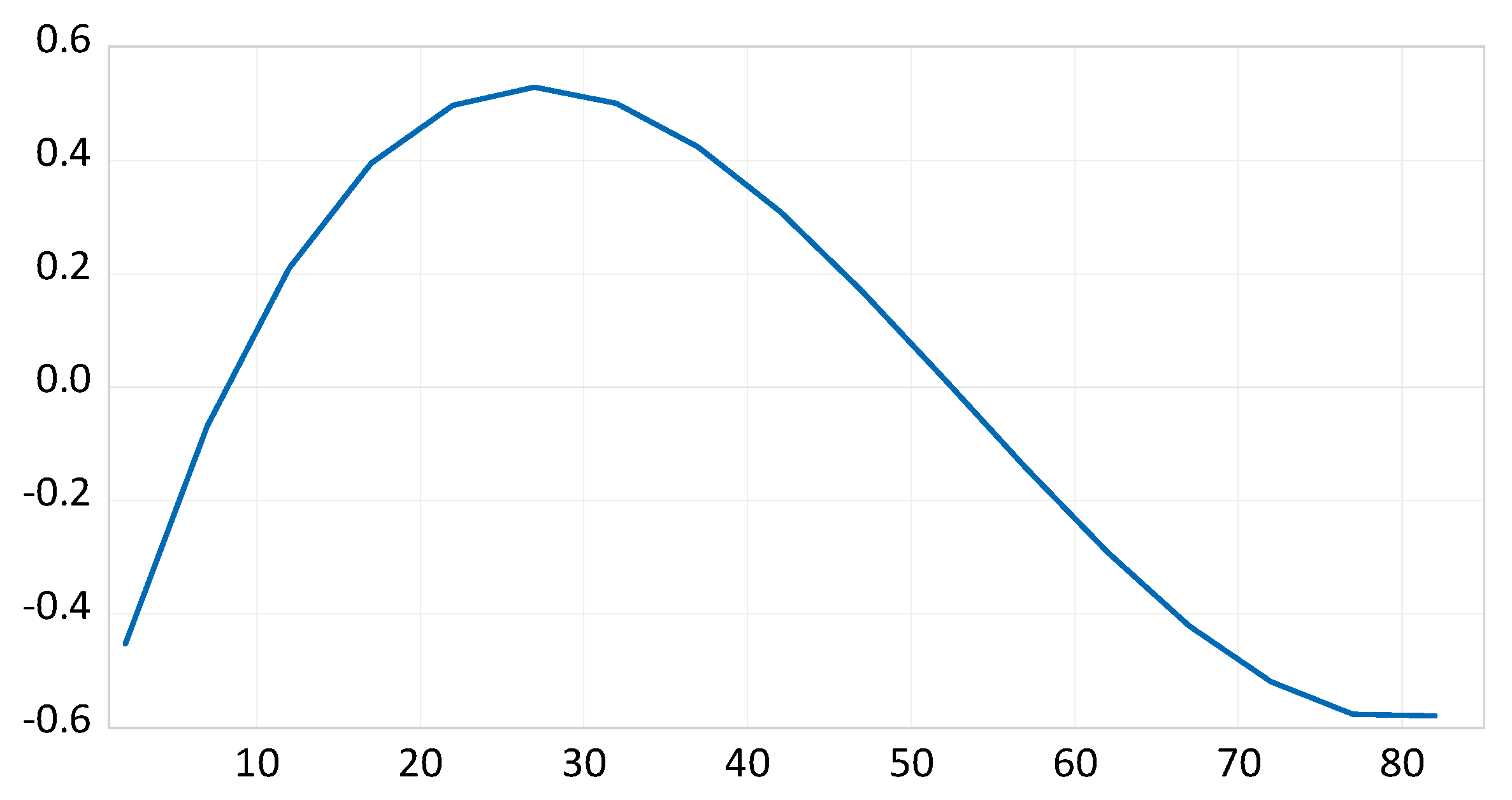
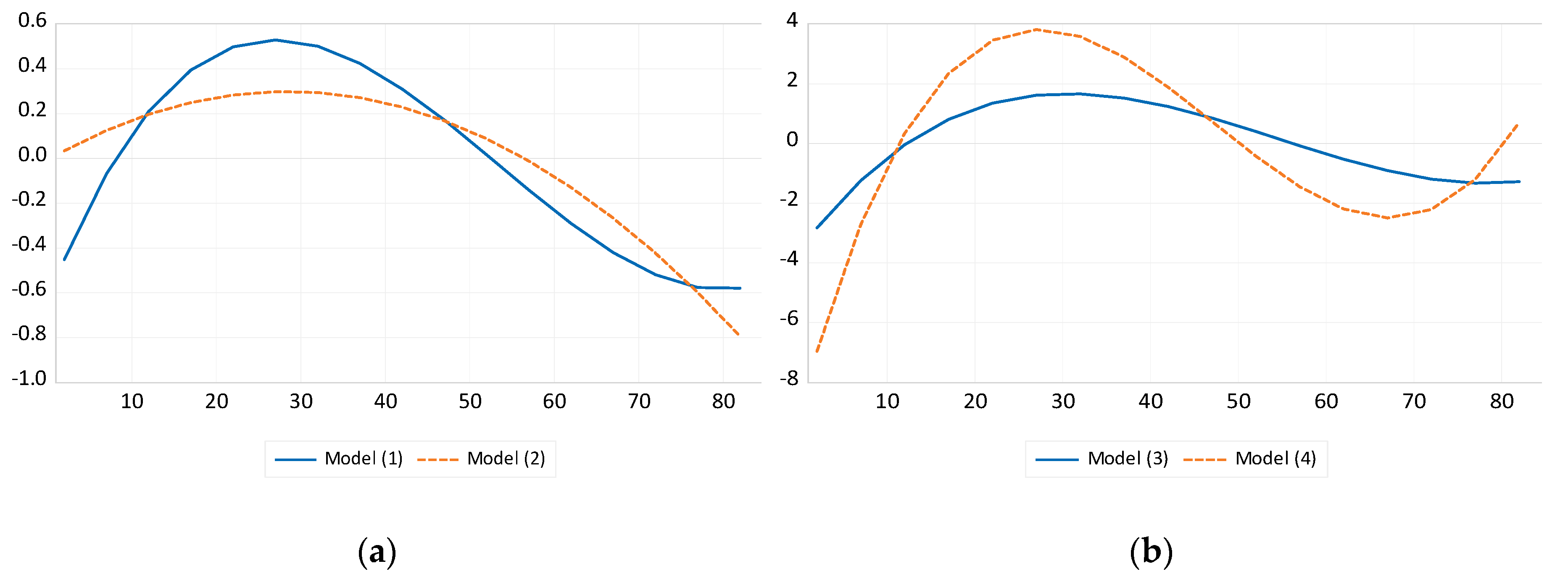
3.1. Modeling the Age Structure Effect
3.2. Data
4. Results
4.1. Panel Unit Root and Cointegration Tests
4.2. Panel Cointegration Regression: Fully-Modified Ordinary Least Squares
4.3. Robustness Check
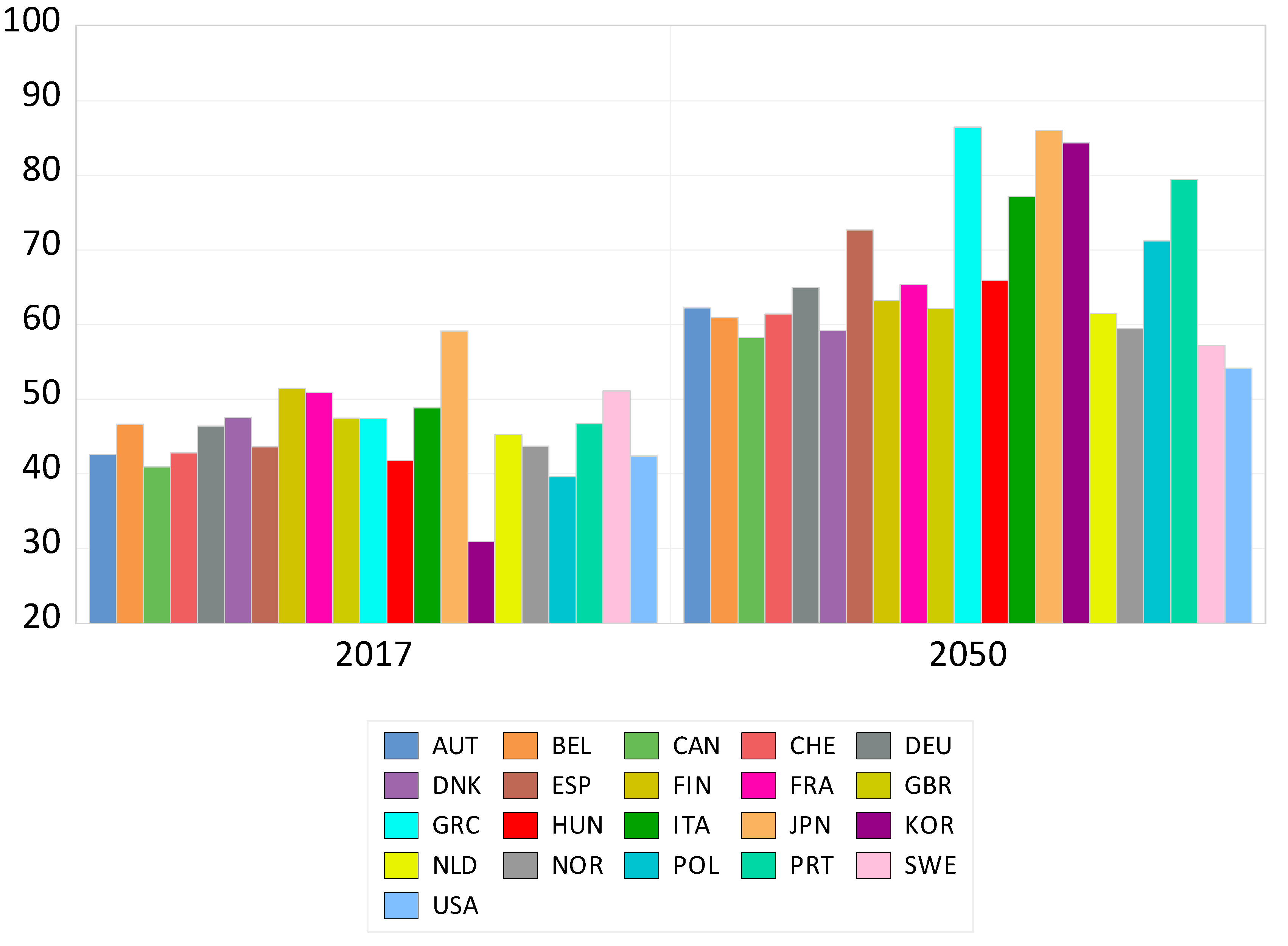
4.4. Projecting GHG Emissions Using the Age Structure Outlook
5. Discussion
6. Conclusions
Supplementary Materials
Author Contributions
Funding
Acknowledgments
Conflicts of Interest
Appendix A
References
- OECD/ITF. Transport CO2 and the Paris Climate Agreement: Reviewing the Impact of Nationally Determined Contibutions; OECD: Paris, France, 2018. [Google Scholar]
- Sims, R.; Schaeffer, R.; Creutzig, F.; Cruz-Núñez, X.; D’agosto, M.; Dimitriu, D.; Figueroa Meza, M.J.; Fulton, L.; Kobayashi, S.; McKinnon, A.; et al. Transport Climate Change 2014: Mitigation of Climate Change; Contribution of Working Group III to the Fifth Assessment Report of the Intergovernmental Panel on Climate Change ed O Edenhofer et al.; Cambridge University Press: Cambridge, UK; New York, NY, USA, 2014; Available online: http://www.ipcc.ch/pdf/assessment-report/ar5/wg3/ipcc_wg3_ar5_chapter8.Pdf (accessed on 1 September 2020).
- International Energy Agency (IEA). Global EV Outlook 2020; IEA: Paris, France, 2020. [Google Scholar]
- Shahbaz, M.; Loganathan, N.; Muzaffar, A.T.; Ahmed, K.; Jabran, M.A. How urbanization affects CO2 emissions in Malaysia? The application of STIRPAT model. Renew. Sustain. Energy Rev. 2016, 57, 83–93. [Google Scholar] [CrossRef] [Green Version]
- González, R.M.; Marrero, G.A. The effect of dieselization in passenger cars emissions for Spanish regions: 1998–2006. Energy Policy 2012, 51, 213–222. [Google Scholar] [CrossRef]
- Rosenbloom, S. Sustainability and automobility among the elderly: An international assessment. Transportation 2001, 28, 375–408. [Google Scholar] [CrossRef]
- Hassan, K.; Salim, R. Population ageing, income growth and CO2 emission: Empirical evidence from high income OECD countries. J. Econ. Stud. 2015, 42, 54–67. [Google Scholar] [CrossRef]
- Schmöcker, J.D.; Quddus, M.A.; Noland, R.B.; Bell, M.G. Mode choice of older and disabled people: A case study of shopping trips in London. J. Transp. Geogr. 2008, 16, 257–267. [Google Scholar] [CrossRef] [Green Version]
- Liddle, B.; Lung, S. Age-structure, urbanization, and climate change in developed countries: Revisiting STIRPAT for disaggregated population and consumption-related environmental impacts. Popul. Environ. 2010, 31, 317–343. [Google Scholar] [CrossRef] [Green Version]
- Schmöcker, J.D.; Quddus, M.A.; Noland, R.B.; Bell, M.G. Estimating trip generation of elderly and disabled people: Analysis of London data. Transp. Res. Rec. 2005, 1924, 9–18. [Google Scholar] [CrossRef]
- Paez, A.; Scott, D.; Potoglou, D.; Kanaroglou, P.; Newbold, K.B. Elderly mobility: Demographic and spatial analysis of trip making in the Hamilton CMA, Canada. Urban Stud. 2007, 44, 123–146. [Google Scholar] [CrossRef]
- Fair, R.; Dominguez, K. Effects of the changing US demographic structure on macroeconomic equations. Am. Econ. Rev. 1991, 81, 1276–1294. [Google Scholar]
- Juselius, J.; Takáts, E. The Enduring Link between Demography and Inflation (No. 722); Bank for International Settlements: Basel, Switzerland, 2018. [Google Scholar]
- Jo, H.H.; Jang, M.; Kim, J. How Population Age Distribution Affect Future Electricity Demand in Korea: Applying Population Polynomial Function. Energies 2020, 13, 5360. [Google Scholar] [CrossRef]
- Pedroni, P. Fully modified OLS for heterogeneous cointegrated panels. Adv. Econom. 2000, 15, 93–130. [Google Scholar]
- Mustapa, S.I.; Bekhet, H.A. Investigating factors affecting CO2 emissions in Malaysian road transport sector. Int. J. Energy Econ. Policy 2015, 5, 1073–1083. [Google Scholar]
- Chai, J.; Yang, Y.; Wang, S.; Lai, K.K. Fuel efficiency and emission in China’s road transport sector: Induced effect and rebound effect. Technol. Forecast. Soc. Chang. 2016, 112, 188–197. [Google Scholar] [CrossRef]
- Schipper, L. Automobile use, fuel economy and CO2 emissions in industrialized countries: Encouraging trends through 2008? Transp. Policy 2011, 18, 358–372. [Google Scholar] [CrossRef]
- Lakshmanan, T.R.; Han, X. Factors underlying transportation CO2 emissions in the USA: A decomposition analysis. Transp. Res. Part D Transp. Environ. 1997, 2, 1–15. [Google Scholar] [CrossRef]
- Timilsina, G.R.; Shrestha, A. Transport sector CO2 emissions growth in Asia: Underlying factors and policy options. Energy Policy 2009, 37, 4523–4539. [Google Scholar] [CrossRef]
- Wang, W.W.; Zhang, M.; Zhou, M. Using LMDI method to analyze transport sector CO2 emissions in China. Energy 2011, 36, 5909–5915. [Google Scholar] [CrossRef]
- Shahbaz, M.; Khraief, N.; Jemaa, M.M.B. On the causal nexus of road transport CO2 emissions and macroeconomic variables in Tunisia: Evidence from combined cointegration tests. Renew. Sustain. Energy Rev. 2015, 51, 89–100. [Google Scholar] [CrossRef] [Green Version]
- Jones, D.W. How urbanization affects energy-use in developing countries. Energy Policy 1991, 19, 621–630. [Google Scholar] [CrossRef]
- York, R.; Rosa, E.A.; Dietz, T. Footprints on the earth: The environmental consequences of modernity. Am. Sociol. Rev. 2003, 68, 279–300. [Google Scholar] [CrossRef]
- Newman, P.G.; Kenworthy, J.R. Cities and Automobile Dependence: An International Sourcebook; Gower: Brookfield, VT, USA, 1989. [Google Scholar]
- Hilton, F.H.; Levinson, A. Factoring the environmental Kuznets curve: Evidence from automotive lead emissions. J. Environ. Econ. Manag. 1998, 35, 126–141. [Google Scholar] [CrossRef] [Green Version]
- Liddle, B. Demographic dynamics and per capita environmental impact: Using panel regressions and household decompositions to examine population and transport. Popul. Environ. 2004, 26, 23–39. [Google Scholar] [CrossRef]
- Henderson, V. The urbanization process and economic growth: The so-what question. J. Econ. Growth 2003, 8, 47–71. [Google Scholar] [CrossRef]
- Clerides, S.; Zachariadis, T. The effect of standards and fuel prices on automobile fuel economy: An international analysis. Energy Econ. 2008, 30, 2657–2672. [Google Scholar] [CrossRef]
- Xu, B.; Lin, B. Factors affecting carbon dioxide (CO2) emissions in China’s transport sector: A dynamic nonparametric additive regression model. J. Clean. Prod. 2015, 101, 311–322. [Google Scholar] [CrossRef]
- Mustapa, S.I.; Bekhet, H.A. Analysis of CO2 emissions reduction in the Malaysian transportation sector: An optimisation approach. Energy Policy 2016, 89, 171–183. [Google Scholar] [CrossRef]
- Hasan, M.A.; Frame, D.J.; Chapman, R.; Archie, K.M. Emissions from the road transport sector of New Zealand: Key drivers and challenges. Environ. Sci. Pollut. Res. 2019, 26, 23937–23957. [Google Scholar] [CrossRef]
- Oshiro, K.; Masui, T. Diffusion of low emission vehicles and their impact on CO2 emission reduction in Japan. Energy Policy 2015, 81, 215–225. [Google Scholar] [CrossRef]
- Transport & Environment. How Clean are Electric Cars: T&E’s Analysis of Electric Car Lifecycle CO2 Emissions; Transport & Environment: Brussels, Belgium, 2020. [Google Scholar]
- Kim, J.; Lim, H.; Jo, H.H. Do Aging and Low Fertility Reduce Carbon Emissions in Korea? Evidence from IPAT Augmented EKC Analysis. Int. J. Environ. Res. Public Health 2020, 17, 2972. [Google Scholar] [CrossRef] [PubMed]
- Okada, A. Is an increased elderly population related to decreased CO2 emissions from road transportation? Energy Policy 2012, 45, 286–292. [Google Scholar] [CrossRef]
- Liddle, B. Consumption-driven environmental impact and age structure change in OECD countries: A cointegration-STIRPAT analysis. Demogr. Res. 2011, 24, 749–770. [Google Scholar] [CrossRef] [Green Version]
- Weilenmann, M.; Favez, J.Y.; Alvarez, R. Cold-start emissions of modern passenger cars at different low ambient temperatures and their evolution over vehicle legislation categories. Atmos. Environ. 2009, 43, 2419–2429. [Google Scholar] [CrossRef]
- Räty, R.; Carlsson-Kanyama, A. Energy consumption by gender in some European countries. Energy Policy 2010, 38, 646–649. [Google Scholar] [CrossRef]
- Government Office for Science. How Can Transport Provision and Associated Built Environment Infrastructure Be Enhanced and Developed to Support the Mobility Needs of Individuals as They Age; Government Office for Science: London, UK, 2015.
- Eby, D.W.; Molnar, L.J. Older adult safety and mobility: Issues and research needs. Public Work. Manag. Policy 2009, 13, 288–300. [Google Scholar] [CrossRef]
- McGuckin, N.; Srinivasan, N. Journey to Work Trends in the United States and Its Major Metropolitan Areas; FHWA-EP-03; US Department of Transportation, Federal Highway Administration, Office of Planning: Ames, IA, USA, 2003; Volume 58.
- Im, K.S.; Pesaran, M.H.; Shin, Y. Testing for unit roots in heterogeneous panels. J. Econom. 2003, 115, 53–74. [Google Scholar] [CrossRef]
- Pesaran, M.H. A simple panel unit root test in the presence of cross-section dependence. J. Appl. Econom. 2007, 22, 265–312. [Google Scholar] [CrossRef] [Green Version]
- Kao, C. Spurious regression and residual-based tests for cointegration in panel data. J. Econom. 1999, 90, 1–44. [Google Scholar] [CrossRef]
- Kim, J.; Jang, M.; Shin, D. Examining the Role of Population Age Structure upon Residential Electricity Demand: A Case from Korea. Sustainability 2019, 11, 3914. [Google Scholar] [CrossRef] [Green Version]
- Mark, N.C.; Sul, D. Cointegration vector estimation by panel DOLS and long-run money demand. Oxf. Bull. Econ. Stat. 2003, 65, 655–680. [Google Scholar] [CrossRef] [Green Version]
- Arnott, R.D.; Chaves, D.B. Demographic changes, financial markets, and the economy. Financ. Anal. J. 2012, 68, 23–46. [Google Scholar] [CrossRef]
- Department for Transport (DfT). Transport Statistics Great Britain; DfT: London, UK, 2013. Available online: www.gov.uk/government/uploads/system/uploads/attachment_data/file/264679/tsgb-2013.pdf (accessed on 1 September 2020).


| Variable Name | Variable Definition | Unit | Data Source | Range |
|---|---|---|---|---|
| E(Emissions) | Per capita greenhouse gas (GHG) emissions in road transportation | tCO2eq | Internationa Energy Agency (IEA), Enerdata | 2000–2016 (annual) |
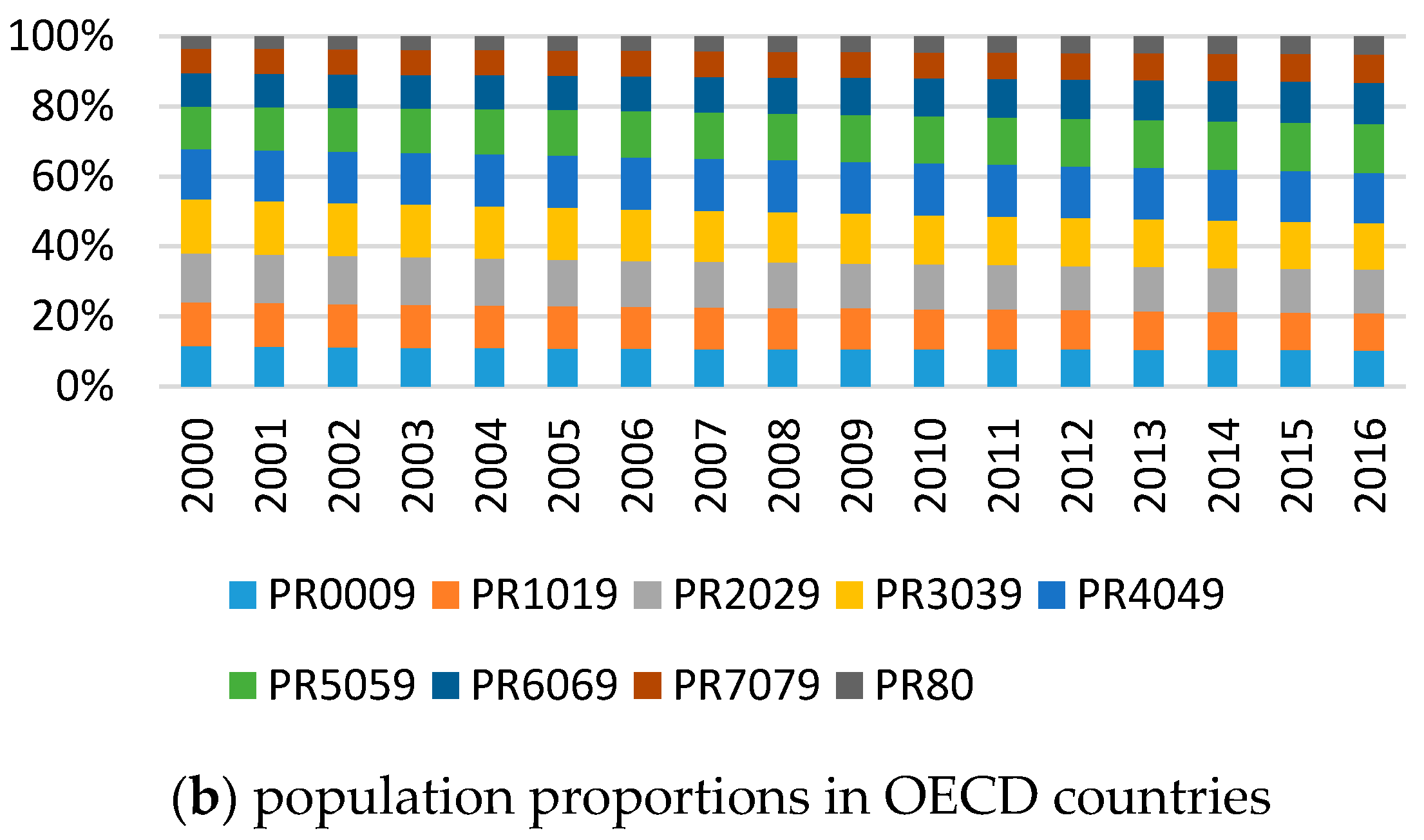
| PR1–PR17 | Proportion of age groups (0–4, 5–9,…, 75–79, over 80) | % | World Bank, Organization for Economic Cooperation and Development (OECD) | |
| Y(Income) | Per capita real gross domestic product (GDP) | 2010 US$ | World Bank | |
| FP(Fuel Price) | Weighted average real price of gasoline and diesel (weighted as a proportion of gasoline and diesel consumption) | 2015 US$/tonnes of oil equivalent (toe) | Adapted from Enerdata | |
| VO(Vehicle Ownership) | Per capita number of registered vehicles | units/person | OECD | |
| PD(Population Density) | Population density | person/km2 | World Bank | |
| UR(Urbanization) | Ratio of urban population | % | World Bank | |
| FE(Fuel Economy) | (annual distance traveled × total registered vehicles)/total fuel consumption | km/L | Odyssee-Mure International Council for Clean Transportation (ICCT) | |
| TV(Transport Volume) | Per capita transport volume of road transportation | million tons/person | OECD | |
| FT (fuel transition) | Ratio of non-conventional fossil fuel consumption in road transportation (percentage of electricity, natural gas, and biofuel use) | % | IEA, Enerdata |
| Variable | Mean | Maximum | Minimum | Standard Deviation | Observation |
|---|---|---|---|---|---|
| E(Emissions) | 2.1 | 5.3 | 0.7 | 0.9 | 357 |
| Y(Income) | 41,655 | 91,566 | 8526 | 17,926 | 357 |
| FP(Fuel Price) | 1660.7 | 2678.0 | 607.8 | 346.7 | 357 |
| VO(Vehicle Ownership) | 0.6 | 0.9 | 0.3 | 0.1 | 352 |
| PD(Population Density) | 169.0 | 525.4 | 3.4 | 145.3 | 357 |
| UR(Urbanization) | 77.3 | 97.9 | 54.4 | 9.8 | 357 |
| FE(Fuel Economy) | 14.0 | 23.8 | 9.5 | 2.2 | 342 |
| TV(Transport Volume) | 3093 | 71,860 | 44 | 11,031 | 296 |
| FT(Fuel Transition) | 2.7 | 16.4 | 0.0 | 2.8 | 357 |
| Model (1) (Benchmark) | Model (2) | Model (3) | Model (4) | ||
|---|---|---|---|---|---|
| Age structure effect | z1 | 0.562 *** | 0.119 ** | 2.256 *** | 6.305 *** |
| z2 (×10) | −0.639 *** | −0.095 *** | −2.375 *** | −7.444 *** | |
| z3 (×) | 0.189 ** | 0.689 *** | 2.466 *** | ||
| Personal transport use | Y | 0.642 *** | 0.647 *** | 0.842 *** | 0.728 *** |
| FP | −0.048 *** | −0.045 *** | −0.098 *** | −0.167 *** | |
| VO | 0.252 *** | 0.239 *** | 0.358 *** | 0.380 *** | |
| Macro transport environment | PD | −0.891 *** | −0.920 *** | −1.004 *** | |
| UR | −0.006 *** | −0.007 *** | −0.002 *** | ||
| FE | −0.075 *** | −0.068 *** | −0.248 *** | ||
| TV | 0.113 *** | 0.121 *** | |||
| FT | −0.009 *** | −0.010 *** | |||
| Wald test (H0: k = 2 vs. H1: k = 3) | 5.27 ** | - | 39.96 *** | 310.11 *** | |
| Wald test (H0: k = 3 vs. H1: k = 4) | 0.83 | - | 263.34 *** | 452.38 *** | |
| F-test of age structure | 140.19 *** | 72.63 *** | 165.11 *** | 385.77 *** | |
| Obs. | 220 | 220 | 316 | 330 | |
| Adj-R2 | 0.984 | 0.984 | 0.985 | 0.977 | |
| Robust (1) | Robust (2) | ||
|---|---|---|---|
| Age structure effect | PR0014 | −0.253 | |
| PR65 | −1.378 *** | ||
| DEPR0014 | −0.059 ** | ||
| DEPR65 | −0.238 *** | ||
| Personal transport use | Y | 0.645 *** | 0.679 *** |
| FP | −0.060 *** | −0.074 *** | |
| VO | 0.244 *** | 0.250 *** | |
| Macro transportenvironment | PD | −1.028 *** | −1.062 *** |
| UR | −0.006 *** | −0.005 *** | |
| FE | −0.014 | −0.006 | |
| TV | 0.110 *** | 0.100 *** | |
| FT | −0.009 *** | −0.009 *** | |
| F-test of age structure | 125.14 *** | 84.98 *** | |
| Obs. | 220 | 220 | |
| Adj-R2 | 0.985 | 0.985 | |
| 2010 | 2017 | 2030 | 2050 | % Change (2017–2050) | Annual % Change (2017–2050) | |
|---|---|---|---|---|---|---|
| Austria | 2.60 | 2.67 | 2.57 | 2.50 | −6.4% | −0.2% |
| Belgium | 2.31 | 2.17 | 2.12 | 2.09 | −3.6% | −0.1% |
| Canada | 4.18 | 3.86 | 3.72 | 3.66 | −5.2% | −0.2% |
| Switzerland | 2.15 | 1.83 | 1.77 | 1.70 | −6.9% | −0.2% |
| Germany | 1.76 | 1.94 | 1.87 | 1.82 | −6.0% | −0.2% |
| Denmark | 2.20 | 1.94 | 1.89 | 1.87 | −3.7% | −0.1% |
| Spain | 1.85 | 1.76 | 1.69 | 1.61 | −8.5% | −0.3% |
| Finland | 2.20 | 1.97 | 1.93 | 1.86 | −5.4% | −0.2% |
| France | 1.83 | 1.82 | 1.77 | 1.76 | −3.4% | −0.1% |
| United Kingdom | 1.76 | 1.74 | 1.69 | 1.65 | −5.2% | −0.2% |
| Greece | 1.70 | 1.34 | 1.21 | 1.05 | −21.7% | −0.7% |
| Hungary | 1.14 | 1.28 | 1.23 | 1.19 | −7.4% | −0.2% |
| Italy | 1.75 | 1.52 | 1.46 | 1.40 | −8.1% | −0.2% |
| Japan | 1.57 | 1.45 | 1.40 | 1.34 | −7.5% | −0.2% |
| Korea, Rep. | 1.67 | 1.91 | 1.74 | 1.57 | −17.9% | −0.6% |
| Netherlands | 1.97 | 1.73 | 1.67 | 1.65 | −4.8% | −0.1% |
| Norway | 1.95 | 1.64 | 1.59 | 1.53 | −6.6% | −0.2% |
| Poland | 1.22 | 1.59 | 1.51 | 1.41 | −11.2% | −0.4% |
| Portugal | 1.67 | 1.54 | 1.47 | 1.39 | −9.9% | −0.3% |
| Sweden | 2.20 | 1.90 | 1.87 | 1.84 | −2.8% | −0.1% |
| United States | 4.76 | 4.48 | 4.36 | 4.28 | −4.5% | −0.1% |
| Average | 2.12 | 2.00 | 1.93 | 1.87 | −6.9% | −0.2% |
Publisher’s Note: MDPI stays neutral with regard to jurisdictional claims in published maps and institutional affiliations. |
© 2020 by the authors. Licensee MDPI, Basel, Switzerland. This article is an open access article distributed under the terms and conditions of the Creative Commons Attribution (CC BY) license (http://creativecommons.org/licenses/by/4.0/).
Share and Cite
Lim, H.; Kim, J.; Jo, H.-H. Population Age Structure and Greenhouse Gas Emissions from Road Transportation: A Panel Cointegration Analysis of 21 OECD Countries. Int. J. Environ. Res. Public Health 2020, 17, 7734. https://doi.org/10.3390/ijerph17217734
Lim H, Kim J, Jo H-H. Population Age Structure and Greenhouse Gas Emissions from Road Transportation: A Panel Cointegration Analysis of 21 OECD Countries. International Journal of Environmental Research and Public Health. 2020; 17(21):7734. https://doi.org/10.3390/ijerph17217734
Chicago/Turabian StyleLim, Hyungwoo, Jaehyeok Kim, and Ha-Hyun Jo. 2020. "Population Age Structure and Greenhouse Gas Emissions from Road Transportation: A Panel Cointegration Analysis of 21 OECD Countries" International Journal of Environmental Research and Public Health 17, no. 21: 7734. https://doi.org/10.3390/ijerph17217734