Classification of Biodegradable Substances Using Balanced Random Trees and Boosted C5.0 Decision Trees


Abstract
:1. Introduction
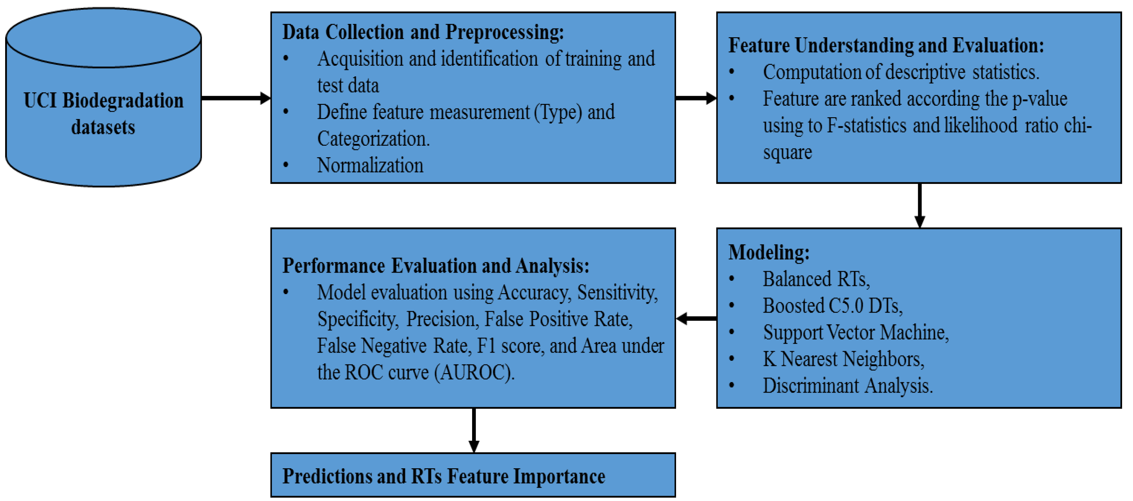
- The data files were obtained from the UCI machine learning repository and grouped into training and test subsets.
- The descriptive statistics were estimated and the predictive importance was evaluated using mixed type p-values based on F-statistics and likelihood ratio chi-squared tests.
- Machine learning models were proposed for the classification of ready-biodegradable substances using balanced RTs and boosted C5.0 DTs models.
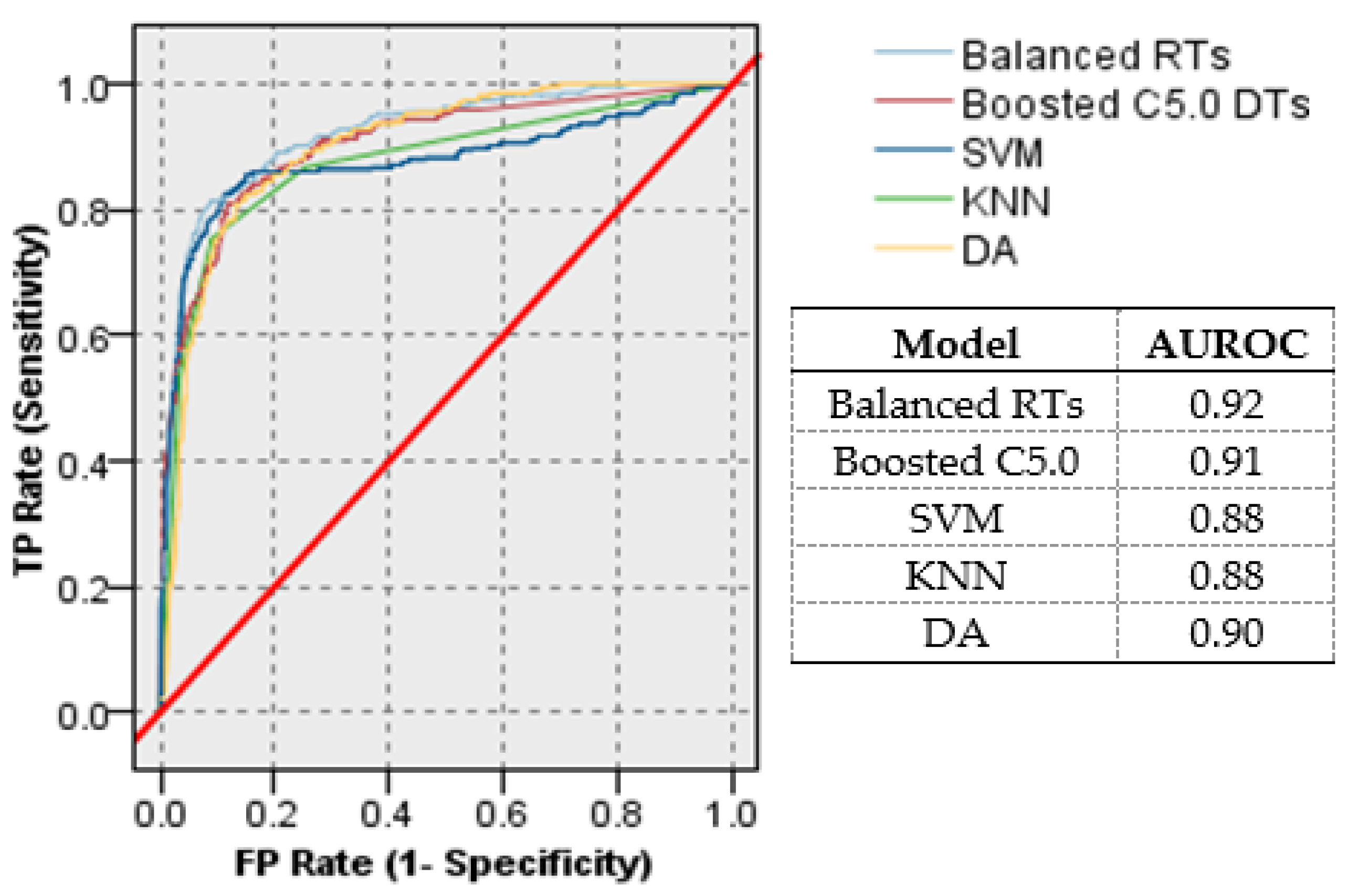
- Classification performance was evaluated in terms of accuracy, sensitivity, specificity, precision, false positive rate, false negative rate, F1 score, receiver operating characteristic (ROC) curve, and the area under the ROC curve (AUROC).
- Experimental results show that the proposed models outperform the classification results provided by the support vector machine (SVM), K-nearest neighbors (KNN), and discrimination analysis (DA).
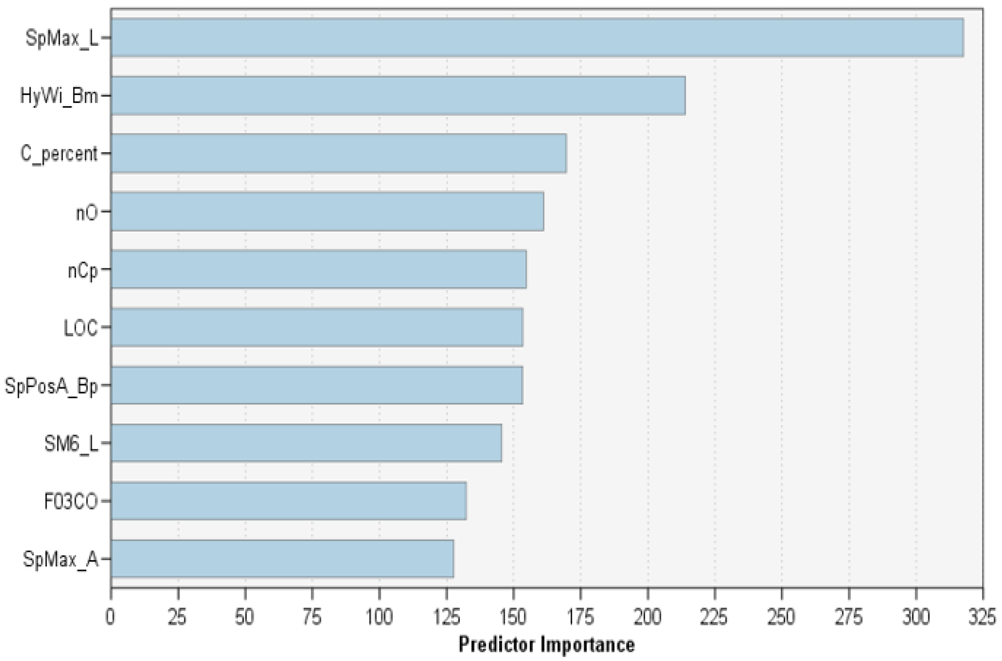
- The top ten molecular descriptors were ranked according to their contributions to the balanced RTs classification process.

| Authors | Dataset | Machine Learning Model | Classification Result |
|---|---|---|---|
| Tang et al. [13] 2020 | A dataset with 171 compounds was collected from the BIOWIN3 and BIOWIN4 programs and a qualitative dataset from BIOWIN 5 and 6 to validate the reliability of their models. | Four QSAR models were developed for predicting primary and ultimate biodegradation rate rating with multiple linear regression (MLR) and support vector regression (SVR) algorithms. | SVR models have satisfactory goodness-of-fit, robustness, and external predictive abilities. |
| Lunghini et al. [14] 2020. | Ready biodegradability dataset (2830 compounds), issued by merging several public data sources. | SVM models with linear and RBF kernels, random forest (RF), and Naïve Bayesian (NB) and their Ensemble. | The proposed models showed good performances in terms of predictive power (Balance Accuracy (BA) = 0.74–0.79) and data coverage (83–91%). |
| Putra et al. [15] 2019 | UCI biodegradation dataset. | Artificial neural networks (ANN) and SVM models were built to predict the ready-biodegradation of a chemical compound. Authors reduced the 41 molecular descriptors using principal components analysis (PCA) into four components | SVM achieved 0.77 accuracy, 0.54 sensitivity, and 0.85 specificity. ANN achieved an accuracy of 0.77, sensitivity of 0.61, and specificity of 0.85. |
| Ballabio et al. [16] 2017. | VEGA, BIOWIN, and Michem datasets, as well as external validation data set | Eight different models: BIOWIN, VEGA, Michem PLS-DA, Michem SVM, Michem KNN, CASE Ultra DTU, Leadscope DTU, and SciQSAR DTU. | VEGA achieved the best non-error rate of 0.88 with a sensitivity of 0.86 and specificity of 0.9. |
| Zhan et al. [17] 2017 | UCI biodegradation dataset. | Naïve Bayes. | AUCs 0.890, 0.921, and 0.901 for training, test and external validation subsets. |
| Rocha, W. F. C., and Sheen [18] 2016. | UCI biodegradation dataset. | PLS_DA with uncertainty estimation. | They achieved sensitivity of 0.88 and specificity of 0.832 for training data, sensitivity of 0.833, and specificity of 0.87 for test data, and sensitivity of 0.80 and specificity of 0.856 for external validation. |
| Fernández et al. [19] 2015. | Four Publicly available datasets: BIOWIN, Cheng et al., Japanese MITI, and Lombardo et al. | QSAR models: BIOWIN5, BIOWIN6, START, and VEGA. | BIOWIN6 achieved the best performance with 0.57 MCC, and the consensus of the four models achieved 0.74 MCC |
| Mansouri et al. [11] 2013. | UCI biodegradation dataset. | KNN, PLS-DA, SVM, consensus 1 and consensus 2 with genetic algorithms. | Best results with consensus 2: training error rate of 0.07, test error rate of 0.09, and external validation error rate of 0.13. |
| Cheng et al. [20] 2012. | MITI and BIOWIN data sets | SVM, kNN, Naïve Bayes, and C4.5 decision tree using four different feature selections CFS, CART, CHAID, and GA | Best AUCs are 0.856, 0.844, and 0.873 for CART-NB, CHAID-SVM, and GASVM-kNN models, respectively |
2. Literature Review
3. Method Pipeline
3.1. Data Collection and Preprocessing
3.2. Feature Understanding and Evaluation
- The -value based on likelihood ratio chi-square is calculated by , where:where is the observed cell frequency and is the expected cell frequency for the cell . That is the likelihood ratio chi-square test evaluates the independence between the feature and the output class that involves the difference between the observed and expected frequencies using the contingency table.
- The -value based on F statistic is calculated by , where:where is the mean of the ith feature, is the mean of ith feature in the jth class, is the variance of the ith feature in the jth class, and is the number of samples in the jth class. The value of F-statistics increases if the distances between classes are large and the distances within classes are small, which makes the predictive power of the feature is large.
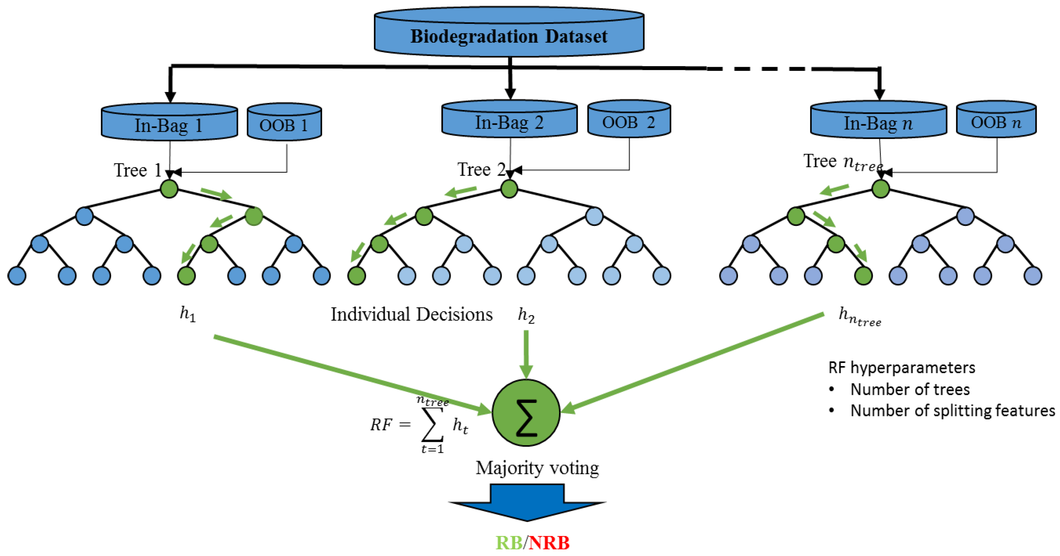
3.3. Balanced Random Trees (RTs)
- Step 1:
- At each decision node, start with all features (.
- Step 2:
- Select randomly features out of the available features (.
- Step 3:
- Find the most important feature among the selected features to partition the node data based on a prespecified splitting criterion (Gini’s diversity index).
- Step 4:
- Split the current node into two descend nodes (binary partitioning) and continue to develop the tree to its maximum expansion (until there is only one sample in every terminal leaf).
- Step 5:
- End and Output trained decision trees (RTs ensemble).
3.3.1. Splitting Criteria
3.3.2. Feature Importance
3.4. Boosted C5.0 DT Model
3.4.1. C5.0 Tree Modeling
3.4.2. C5.0 Cost-Sensitive Tree
3.4.3. C5.0 Boosting Algorithm
- Step 1:
- Initialize the boosting parameters: set the number of trials (10 is a common value), start iteration = 1, and initialize weights ( is the number of training samples)
- Step 2:
- Compute the normalized factors
- Step 3:
- Assign each to the weight of i sample and then generate the tree according to the current weight distribution.
- Step 4:
- Evaluate the error rate of as .
- Step 5:
- If , the trials are closed and set T = t + 1;else if , the trials are terminated and set T = t;else if continue to step 6.
- Step 6:
- Compute .
- Step 7:
- Considering the error rate, adjust the weights using :
- Step 8:
- if t = T, the trials are terminated. Else, set t = T + 1, and go to step 2 to generate the next trial.
4. Experimental Results and Discussion
4.1. Performance Measures
4.2. Balanced RTs Model
4.3. Boosted C5.0 DTs Model
4.4. Model Evaluation and Comparisons
- (1)
- SVM model builds a decision hyperplane with the maximal margin width to divide the feature space linearly into two regions (binary classifier) [40]. In the non-linear situations, the model allows a misclassification slake variable around the margin with a regularization constraint C and applies a kernel function to estimate the necessary computations instead of transforming the data into a higher dimensional feature space. In this study, the radial basis function (RBF) kernel function is selected with only one adjustable parameter ( [41]. The grid search algorithm is applied to find the optimal values of the regulation parameter C and the RBF sigma σ. The C range was set from 1 to 50, and range was set from 0.1 to 10.0. Using all features, we obtained general accuracies of 0.95 and 0.88 for the training and test subsets, respectively, with a formation of C = 1 and σ = 8.7. On the other hand, using only the recommended 14 features as in Table 2, the results were 89.25% and 86.6%, respectively, with C = 1 and σ = 9.1. That is, the SVM accuracies of the training and test subsets are better when using all features. These results are better than those recorded by SVM in the original work in [11] as shown in Table 1.
- (2)
- KNN model is based on an intuitive idea that the data samples of the same class should be nearer to each other in the feature space [42]. The model classifies any new sample in three steps. Firstly, the model computes its distance from each of the training samples using a certain distance function. Second, the model selects K number of training samples that have the smallest distances with this new sample. These K samples constitute its neighbors. Finally, the model assigns this new sample to the class to which the largest number of these neighbors belong. Both the number of neighbors K and the distance function play critical roles in the success of this model. In this study, a grid search was applied to find the optimal values of K and the distance function. The K range was set from 3 to 15 while the distance function can be Euclidean or City block distance functions. Using all features, we obtained accuracies of 0.91 and 0.86 for the training and test subsets, respectively, with K = 3 and Euclidean distance. While using only the recommended 12 features, the results were 0.92 and 0.86 with K = 3 and Euclidean distance. In this case, the KNN classification accuracies of the training and testing data are better when using the recommended 12 features and are better than the results in [11] as seen in Table 1.
- (3)
- DA model works to find a linear combination of features that distinguish or separate two or more classes of objects. The resulting combination can be used as a linear classifier, or more commonly, to reduce dimensions before subsequent classification [43]. The model works only with continuous input features and categorical outputs. It is assumed that the input features have normal distributions. The violations of the normality assumption are not fatal as long as nonnormality is caused by skewness and not by outliers [23]. If these assumptions are met, DA gives better results. The model requires the determination of methods to compute prior probabilities methods and the covariance matrix. The prior probabilities determine whether the classification coefficients are computed for a priori knowledge of class membership. There are two options: equal probabilities or according to class sizes. The covariance matrix can be estimated within-groups covariance matrix or based on a separate-classes covariance matrix. Using all features, we obtained a classification accuracy of 0.87 and 0.84 for the training and test subsets, respectively. While using only the recommended 23 features, the results were 0.86 and 0.86 for the training and test subsets, respectively. In both experiments, the prior probabilities were computed from the class sizes and the covariance matrix was computed using separate classes. Using the 23 features, the current DA results are similar for the training subset and slightly better for the test subset to those obtained using PLS-DA in [11].
4.5. Model Evaluation Using (ROC) Curves
5. Conclusions
Supplementary Materials
Author Contributions
Funding
Acknowledgments
Conflicts of Interest
References
- Tropsha, A. Best Practices for QSAR Model Development, Validation, and Exploitation. Mol. Inform. 2010, 29, 476–488. [Google Scholar] [CrossRef] [PubMed]
- Roberto, T.; Consonni, V. Handbook of Molecular Descriptors; John Wiley & Sons: Hoboken, NJ, USA, 2008; Volume 11. [Google Scholar]
- Yee, L.C.; Wei, Y.C. Current Modeling Methods Used in QSAR/QSPR. In Statistical Modelling of Molecular Descriptors in QSAR/QSPR; John Wiley & Sons: Hoboken, NJ, USA, 2012; Volume 2, pp. 1–31. [Google Scholar]
- Grisoni, F.; Ballabio, D.; Todeschini, R.; Consonni, V. Molecular descriptors for structure-activity applications: A hands-on approach. In Computational Toxicology; Humana Press: New York, NY, USA, 2018; pp. 3–53. [Google Scholar]
- Joloudari, J.H.; Joloudari, E.H.; Saadatfar, H.; GhasemiGol, M.; Razavi, S.M.; Mosavi, A.; Nabipour, N.; Band, S.S.; Nadai, L. Coronary Artery Disease Diagnosis; Ranking the Significant Features Using a Random Trees Model. Int. J. Environ. Res. Public Health 2020, 17, 731. [Google Scholar] [CrossRef] [PubMed] [Green Version]
- Vanus, J.; Koziorek, J.; Bilik, P. Novel Proposal for Prediction of CO2 Course and Occupancy Recognition in Intelligent Buildings within IoT. Energies 2019, 12, 4541. [Google Scholar] [CrossRef] [Green Version]
- Olson, M. Essays on Random Forest Ensembles. Ph.D. Thesis, University of Pennsylvania, Philadelphia, PA, USA, 2018. Available online: https://repository.upenn.edu/cgi/viewcontent.cgi?article=4519&context=edissertations (accessed on 1 August 2020).
- Rajeswari, S.; Suthendran, K. C5.0: Advanced Decision Tree (ADT) classification model for agricultural data analysis on cloud. Comput. Electron. Agric. 2019, 156, 530–539. [Google Scholar] [CrossRef]
- Naghibi, S.A.; Naghibi, S.A.; Kalantar, B.; Pradhan, B. Groundwater potential mapping using C5.0, random forest, and multivariate adaptive regression spline models in GIS. Environ. Monit. Assess. 2018, 190, 149. [Google Scholar] [CrossRef]
- Elsalamony, H.A.; Elsayad, A.M. Bank direct marketing based on neural network and C5. 0 Models. Int. J. Eng. Adv. Technol. IJEAT 2013, 2, 392–400. [Google Scholar]
- Mansouri, K.; Ringsted, T.; Ballabio, D.; Todeschini, R.; Consonni, V. Quantitative Structure–Activity Relationship Models for Ready Biodegradability of Chemicals. J. Chem. Inf. Model. 2013, 53, 867–878. [Google Scholar] [CrossRef]
- Sun, Y.; Wong, A.K.C.; Kamel, M.S. Classification of Imbalanced Data: A Review. Int. J. Pattern Recognit. Artif. Intell. 2009, 23, 687–719. [Google Scholar] [CrossRef]
- Tang, W.; Li, Y.; Yu, Y.; Wang, Z.; Xu, T.; Chen, J.; Lin, J.; Li, X. Development of models predicting biodegradation rate rating with multiple linear regression and support vector machine algorithms. Chemosphere 2020, 253, 126666. [Google Scholar] [CrossRef]
- Lunghini, F.; Gilles, M.; Gantzer, P.; Azam, P.; Horvath, D.; Van Miert, E.; Varnek, A. Modelling of ready biodegradability based on combined public and industrial data sources. SAR QSAR Environ. Res. 2020, 31, 171–186. [Google Scholar] [CrossRef]
- Putra, R.I.D.; Maulana, A.L.; Saputro, A.G. Study on building machine learning model to predict biodegradable-ready materials. In AIP Conference Proceedings; AIP Publishing LLC: Melville, NY, USA, 2019; Volume 2088, p. 060003. [Google Scholar]
- Ballabio, D.; Biganzoli, F.; Todeschini, R.; Consonni, V. Qualitative consensus of QSAR ready biodegradability predictions. Toxicol. Environ. Chem. 2017, 99, 1193–1216. [Google Scholar] [CrossRef]
- Zhan, Z.; Li, L.; Tian, S.; Zhen, X.; Li, Y. Prediction of chemical biodegradability using computational methods. Mol. Simul. 2017, 43, 1277–1290. [Google Scholar] [CrossRef]
- Rocha, W.F.C.; Sheen, D.A. Classification of biodegradable materials using QSAR modelling with uncertainty estimation. SAR QSAR Environ. Res. 2016, 27, 799–811. [Google Scholar] [CrossRef] [PubMed]
- Fernández, A.; Rallo, R.; Giralt, F.; Fernández, A. Prioritization of in silico models and molecular descriptors for the assessment of ready biodegradability. Environ. Res. 2015, 142, 161–168. [Google Scholar] [CrossRef]
- Cheng, F.; Ikenaga, Y.; Zhou, Y.; Yu, Y.; Li, W.; Shen, J.; Du, Z.; Chen, L.; Xu, C.; Liu, G.; et al. In Silico Assessment of Chemical Biodegradability. J. Chem. Inf. Model. 2012, 52, 655–669. [Google Scholar] [CrossRef]
- Marín-Ortega, P.M.; Dmitriyev, V.; Abilov, M.; Gómez, J.M. ELTA: New Approach in Designing Business Intelligence Solutions in Era of Big Data. Procedia Technol. 2014, 16, 667–674. [Google Scholar] [CrossRef] [Green Version]
- Song, Y.-Y.; Lu, Y. Decision tree methods: Applications for classification and prediction. Shanghai Arch. Psychiatry 2015, 27, 130. [Google Scholar]
- IBM. IBM SPSS Modeler 18 Algorithms Guide; IBM: Armonk, NY, USA; Available online: Ftp://public.dhe.ibm.com/software/analytics/spss/documentation/modeler/18.0/en/AlgorithmsGuide.pdf (accessed on 1 August 2020).
- Kuhn, M.; Johnson, K. Classification Trees and Rule-Based Models. In Applied Predictive Modeling; Springer: New York, NY, USA, 2013; pp. 369–413. [Google Scholar]
- Jain, D.; Singh, V. Feature selection and classification systems for chronic disease prediction: A review. Egypt. Inform. J. 2018, 19, 179–189. [Google Scholar] [CrossRef]
- Ziegler, A.; König, I.R. Mining data with random forests: Current options for real-world applications. Wiley Interdiscip. Rev. Data Min. Knowl. Discov. 2014, 4, 55–63. [Google Scholar] [CrossRef]
- Khalilia, M.; Chakraborty, S.; Popescu, M. Predicting disease risks from highly imbalanced data using random forest. BMC Med. Inform. Decis. Mak. 2011, 11, 51. [Google Scholar] [CrossRef] [Green Version]
- Kuhn, M. Classification Using C5.0 UseR! 2013; Pfizer Global R&D: Groton, CT, USA, 2013. [Google Scholar]
- Quinlan, J.R. Data Mining Tools See5 and C5.0. 2004. Available online: http://www.rulequest.com/see5-info.html (accessed on 3 August 2020).
- Hassoon, M.; Kouhi, M.S.; Zomorodi-Moghadam, M.; Abdar, M. Rule Optimization of Boosted C5.0 Classification Using Genetic Algorithm for Liver disease Prediction. In Proceedings of the 2017 International Conference on Computer and Applications (ICCA), Doha, UAE, 6–7 September 2017; pp. 299–305. [Google Scholar]
- Saeed, M.S.; Mustafa, M.W.; Sheikh, U.U.; Jumani, T.A.; Khan, I.; Atawneh, S.H.; Hamadneh, N.N. An Efficient Boosted C5.0 Decision-Tree-Based Classification Approach for Detecting Non-Technical Losses in Power Utilities. Energies 2020, 13, 3242. [Google Scholar] [CrossRef]
- Pang, S.-L.; Gong, J.-Z. C5.0 Classification Algorithm and Application on Individual Credit Evaluation of Banks. Syst. Eng. Theory Pract. 2009, 29, 94–104. [Google Scholar] [CrossRef]
- Weiss, G.M.; McCarthy, K.; Zabar, B. Cost-sensitive learning vs. sampling: Which is best for handling unbalanced classes with unequal error costs? Dmin 2007, 7, 24. [Google Scholar]
- Robert, E.S.; Freund, Y. Boosting: Foundations and Algorithms; The MIT Press: Cambridge, MA, USA, 2013. [Google Scholar]
- Abdar, M.; Zomorodi-Moghadam, M.; Das, R.; Ting, I.-H. Performance analysis of classification algorithms on early detection of liver disease. Expert Syst. Appl. 2017, 67, 239–251. [Google Scholar] [CrossRef]
- Alizadeh, S.; Ghazanfari, M.; Teimorpour, B. Data Mining and Knowledge Discovery; Iran University of Science and Technology: Tehran, Iran, 2011. [Google Scholar]
- Tharwat, A. Classification assessment methods. Appl. Comput. Inform. 2020. [Google Scholar] [CrossRef]
- Park, Y.; Ho, J. Tackling Overfitting in Boosting for Noisy Healthcare Data. IEEE Trans. Knowl. Data Eng. 2019. [Google Scholar] [CrossRef]
- Jiang, F.; Jiang, Y.; Zhi, H.; Dong, Y.; Li, H.; Ma, S.; Wang, Y.; Dong, Q.; Shen, H.; Wang, Y. Artificial intelligence in healthcare: Past, present and future. Stroke Vasc. Neurol. 2017, 2, 230–243. [Google Scholar] [CrossRef]
- Cortes, C.; Vapnik, V. Support-vector networks. Mach. Learn. 1995, 20, 273–297. [Google Scholar] [CrossRef]
- Luts, J.; Ojeda, F.; Van De Plas, R.; De Moor, B.; Van Huffel, S.; Suykens, J.A.K. A tutorial on support vector machine-based methods for classification problems in chemometrics. Anal. Chim. Acta 2010, 665, 129–145. [Google Scholar] [CrossRef]
- Zhang, S.; Li, X.; Zong, M.; Zhu, X.; Wang, R. Efficient kNN Classification with Different Numbers of Nearest Neighbors. IEEE Trans. Neural Netw. Learn. Syst. 2017, 29, 1774–1785. [Google Scholar] [CrossRef]
- Tharwat, A.; Gaber, T.; Ibrahim, A.; Hassanien, A.E. Linear discriminant analysis: A detailed tutorial. AI Commun. 2017, 30, 169–190. [Google Scholar] [CrossRef] [Green Version]
- Bowers, A.J.; Zhou, X. Receiver Operating Characteristic (ROC) Area under the Curve (AUC): A Diagnostic Measure for Evaluating the Accuracy of Predictors of Education Outcomes. J. Educ. Stud. Placed Risk (JESPAR) 2019, 24, 20–46. [Google Scholar] [CrossRef]


| Descriptor | Definition | Selecting Model | Type | Min | Max | Mean | Std. Dev 1 | Mode 2 | Unique 3 | Importance |
|---|---|---|---|---|---|---|---|---|---|---|
| B01[C-Br] | Presence/absence of C−Br at topological distance 1 | PLS-DA | Flag | 0 | 1 | - | - | 0 | 2 | 1.0 |
| B03[C-Cl] | Presence/absence of C−Cl at topological distance 3 | PLS-DA | Flag | 0 | 1 | - | - | 0 | 2 | 1.0 |
| B04[C-Br] | Presence/absence of C−Br at topological distance 4 | PLS-DA | Flag | 0 | 1 | - | - | 0 | 2 | 1.0 |
| C% | Percentage of C atoms | KNN,PLS-DA | Continuous | 0.0 | 62.5 | 37.5 | 9.1 | 33.3 | - | 1.0 |
| C-026 | R−CX−R | SVM | Ordinal | 0 | 12 | - | - | 0 | 12 | 1.0 |
| F01[N-N] | Frequency of N−N at topological distance 1 | KNN | Ordinal | 0 | 3 | - | - | 0 | 4 | 1.0 |
| F02[C-N] | Frequency of C−N at topological distance 2 | SVM | Ordinal | 0 | 24 | - | - | 0 | 22 | 1.0 |
| F03[C-N] | Frequency of C−N at topological distance 3 | KNN | Ordinal | 0 | 44 | - | - | 0 | 28 | 1.0 |
| F03[C-O] | Frequency of C−O at topological distance 3 | PLS-DA | Ordinal | 0 | 42 | - | - | 0 | 33 | 1.0 |
| F04CN | F04[C-N] frequency of C−N at topological distance 4 2D atom pairs | KNN,PLS-DA | Ordinal | 0 | 36 | - | - | 0 | 25 | 1.0 |
| HyWi_B(m) | Hyper-Wiener-like index (log function) from Burden matrix weighted by mass | PLS-DA | Continuous | 1.5 | 6.3 | 3.6 | 0.6 | 3.6 | - | 1.0 |
| J_Dz(e) | Balaban-like index from Barysz matrix weighted by Sanderson electronegativity | KNN | Continuous | 0.8 | 9.2 | 3.0 | 0.9 | 2.0 | - | 0.9 |
| LOC | Lopping centric index | PLS-DA | Continuous | 0.0 | 4.5 | 1.4 | 0.8 | 0.0 | - | 1.0 |
| Me | Mean atomic Sanderson electronegativity (scaled on Carbon atom) | PLS-DA | Continuous | 1.0 | 1.3 | 1.0 | 0.0 | 1.0 | - | 1.0 |
| Mi | Mean first ionization potential (scaled on carbon atom) | PLS-DA | Continuous | 1.0 | 1.4 | 1.1 | 0.0 | 1.13 | - | 1.0 |
| N-073 | Ar2NH/Ar3N/Ar2N−Al/R···N···R | PLS-DA | Ordinal | 0 | 3 | - | - | 0.0 | 4 | 1.0 |
| nArCOOR | Number of esters (aromatic) | SVM | Ordinal | 0 | 4 | - | - | 0.0 | 5 | 1.0 |
| nArNO2 | Number of nitro groups (aromatic) | PLS-DA | Ordinal | 0 | 4 | - | - | 0.0 | 5 | 1.0 |
| nCb- | Number of substituted benzene C(sp2) | KNN,SVM | Ordinal | 0 | 18 | - | - | 0.0 | 16 | 1.0 |
| nCIR | Number of circuits | PLS-DA | Ordinal | 0 | 147 | - | - | 1.0 | 22 | 1.0 |
| nCp | Number of terminal primary C(sp3) | KNN | Ordinal | 0 | 24 | - | - | 0.0 | 15 | 1.0 |
| nCrt | Number of ring tertiary C(sp3) | SVM | Ordinal | 0 | 8 | - | - | 0.0 | 9 | 1.0 |
| nCRX3 | Number of CRX3 | PLS-DA | Ordinal | 0 | 3 | - | - | 0 | 4 | 1.0 |
| nHDon | Number of donor atoms for H-bonds (N and O) | SVM | Ordinal | 0 | 16 | - | - | 0 | 11 | 1.0 |
| nHM | Number of heavy atoms | KNN | Ordinal | 0 | 12 | - | - | 0 | 11 | 1.0 |
| nN | Number of nitrogen atoms | SVM | Ordinal | 0 | 10 | - | - | 0 | 11 | 1.0 |
| nN-N | Number of N hydrazines | PLS-DA,SVM | Ordinal | 0 | 2 | - | - | 0 | 3 | 1.0 |
| nO | Number of oxygen atoms | KNN,PLS-DA | Ordinal | 0 | 18 | - | - | 0 | 15 | 1.0 |
| NssssC | Number of atoms of type ssssC atom-type | KNN,SVM | Ordinal | 0 | 16 | - | - | 0 | 14 | 1.0 |
| nX | Number of halogen atoms | SVM | Ordinal | 0 | 33 | - | - | 0 | 20 | 1.0 |
| Psi_i_1d | Intrinsic state pseudoconnectivity index−type 1d | PLS-DA | Continuous | 1−.1 | 1.1 | 0.0 | 0.2 | 0.0 | - | 0.3 |
| Psi_i_A | Intrinsic state pseudoconnectivity index--type S average | SVM | Continuous | 1.5 | 5.8 | 2.5 | 0.7 | 2.8 | - | 0.7 |
| SdO | Sum of dO E-states | PLS-DA | Continuous | 0.0 | 95.1 | 10.3 | 13.8 | 0.0 | - | 1.0 |
| SdssC | Sum of dssC E-states | KNN | Continuous | 7−.6 | 4.7 | 0−.2 | 0.8 | 0.0 | - | 0.9 |
| SM6_B(m) | Spectral moment of order 6 from Burden matrix weighted by mass | SVM | Continuous | 4.7 | 17.2 | 8.8 | 1.4 | 8.6 | - | 1.0 |
| SM6_L | Spectral moment of order 6 from Laplace matrix | PLS-DA | Continuous | 4.2 | 12.7 | 10.1 | 1.0 | 8.6 | - | 1.0 |
| SpMax_A | Leading eigenvalue from adjacency matrix (Lovasz−Pelikan index) | PLS-DA | Continuous | 1.0 | 2.9 | 2.2 | 0.2 | 2.0 | - | 1.0 |
| SpMax_B(m) | Leading eigenvalue from Burden matrix weighted by mass | SVM | Continuous | 2.2 | 17.6 | 4.0 | 1.2 | 6.9 | - | 1.0 |
| SpMax_L | Leading eigenvalue from Laplace matrix | KNN,PLS-DA,SVM | Continuous | 2.0 | 6.5 | 4.8 | 0.6 | 4.7 | - | 1.0 |
| SpPosA_B(p) | Normalized spectral positive sum from Burden matrix weighted by polarizability | PLS-DA | Continuous | 0.9 | 1.6 | 1.2 | 0.1 | 1.3 | - | 1.0 |
| TI2_L | Second Mohar index from Laplace matrix | PLS-DA | Continuous | 0.4 | 17.8 | 3.0 | 2.3 | 1.5 | - | 1.0 |
| Model | Sensitivity | Specificity | Accuracy | Precision | F1-Score | FPR | FNR |
|---|---|---|---|---|---|---|---|
| RTs | 0.75 | 0.95 | 0.89 | 0.86 | 0.80 | 0.05 | 0.25 |
| Balanced RTs | 0.80 | 0.92 | 0.89 | 0.82 | 0.81 | 0.08 | 0.20 |
| Molecular Descriptor | Definition | DRAGON Block |
|---|---|---|
| SpMax_L | leading eigenvalue from Laplace matrix | 2D matrix-based |
| HyWi_B(m) | hyper-Wiener-like index (log function) from Burden matrix weighted by mass | 2D matrix-based |
| C% | percentage of C atoms | constitutional indices |
| nO | number of oxygen atoms | constitutional indices |
| nCp | number of terminal primary C(sp3) | functional group counts |
| LOC | lopping centric index | topological indices |
| SpPosA_B(p) | normalized spectral positive sum from Burden matrix weighted by polarizability | 2D matrix-based |
| SM6_L | spectral moment of order 6 from Laplace matrix | 2D matrix-based |
| F03[C-N] | frequency of C−N at topological distance 3 | 2D atom pairs |
| SpMax_A | leading eigenvalue from adjacency matrix (Lovasz−Pelikan index) | 2D matrix-based |
| Model | Sensitivity | Specificity | Accuracy | Precision | F1-Score | FPR | FNR |
|---|---|---|---|---|---|---|---|
| Boosted C5.0 DTs | 0.77 | 0.93 | 0.88 | 0.82 | 0.79 | 0.07 | 0.23 |
| Boosted C5.0 DTs with misclassification cost matrix | 0.81 | 0.88 | 0.86 | 0.73 | 0.77 | 0.12 | 0.19 |
| Model | Sensitivity | Specificity | Accuracy | Precision | F1-Score | FPR | FNR |
|---|---|---|---|---|---|---|---|
| Balanced RTs | 0.80 | 0.93 | 0.89 | 0.82 | 0.81 | 0.08 | 0.20 |
| Boosted C5.0 DTs with misclassification cost matrix | 0.81 | 0.88 | 0.86 | 0.73 | 0.77 | 0.13 | 0.19 |
| SVM | 0.73 | 0.94 | 0.88 | 0.85 | 0.79 | 0.06 | 0.27 |
| KNN | 0.75 | 0.91 | 0.86 | 0.78 | 0.77 | 0.09 | 0.25 |
| DA | 0.73 | 0.91 | 0.86 | 0.77 | 0.75 | 0.09 | 0.27 |
Publisher’s Note: MDPI stays neutral with regard to jurisdictional claims in published maps and institutional affiliations. |
© 2020 by the authors. Licensee MDPI, Basel, Switzerland. This article is an open access article distributed under the terms and conditions of the Creative Commons Attribution (CC BY) license (http://creativecommons.org/licenses/by/4.0/).
Share and Cite
Elsayad, A.M.; Nassef, A.M.; Al-Dhaifallah, M.; Elsayad, K.A. Classification of Biodegradable Substances Using Balanced Random Trees and Boosted C5.0 Decision Trees. Int. J. Environ. Res. Public Health 2020, 17, 9322. https://doi.org/10.3390/ijerph17249322
Elsayad AM, Nassef AM, Al-Dhaifallah M, Elsayad KA. Classification of Biodegradable Substances Using Balanced Random Trees and Boosted C5.0 Decision Trees. International Journal of Environmental Research and Public Health. 2020; 17(24):9322. https://doi.org/10.3390/ijerph17249322
Chicago/Turabian StyleElsayad, Alaa M., Ahmed M. Nassef, Mujahed Al-Dhaifallah, and Khaled A. Elsayad. 2020. "Classification of Biodegradable Substances Using Balanced Random Trees and Boosted C5.0 Decision Trees" International Journal of Environmental Research and Public Health 17, no. 24: 9322. https://doi.org/10.3390/ijerph17249322