The Impact of Environmental Conditions on Urban Eco-Sustainable Total Factor Productivity: A Case Study of 21 Cities in Guangdong Province, China


Abstract
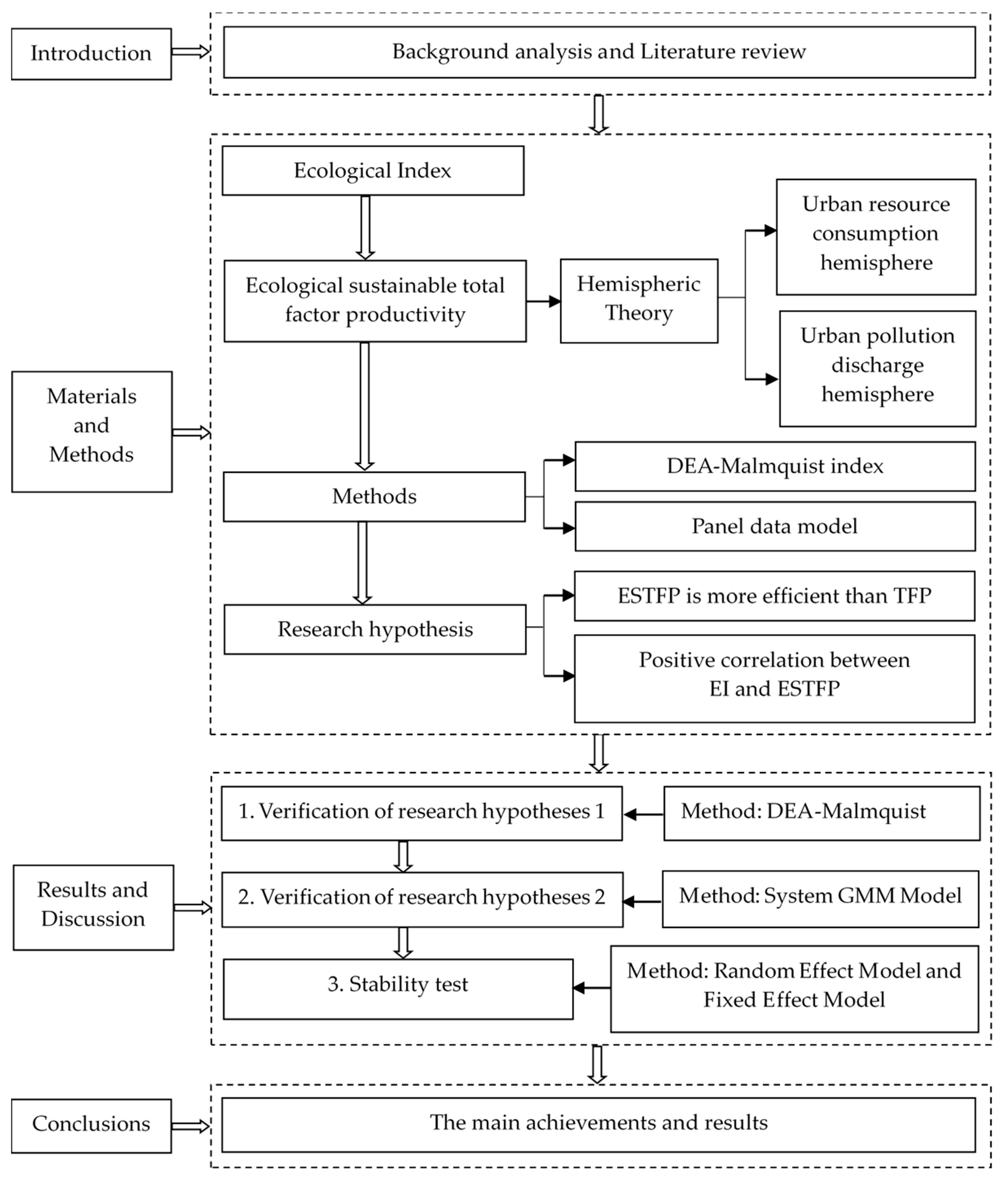
:1. Introduction
2. Materials and Methods
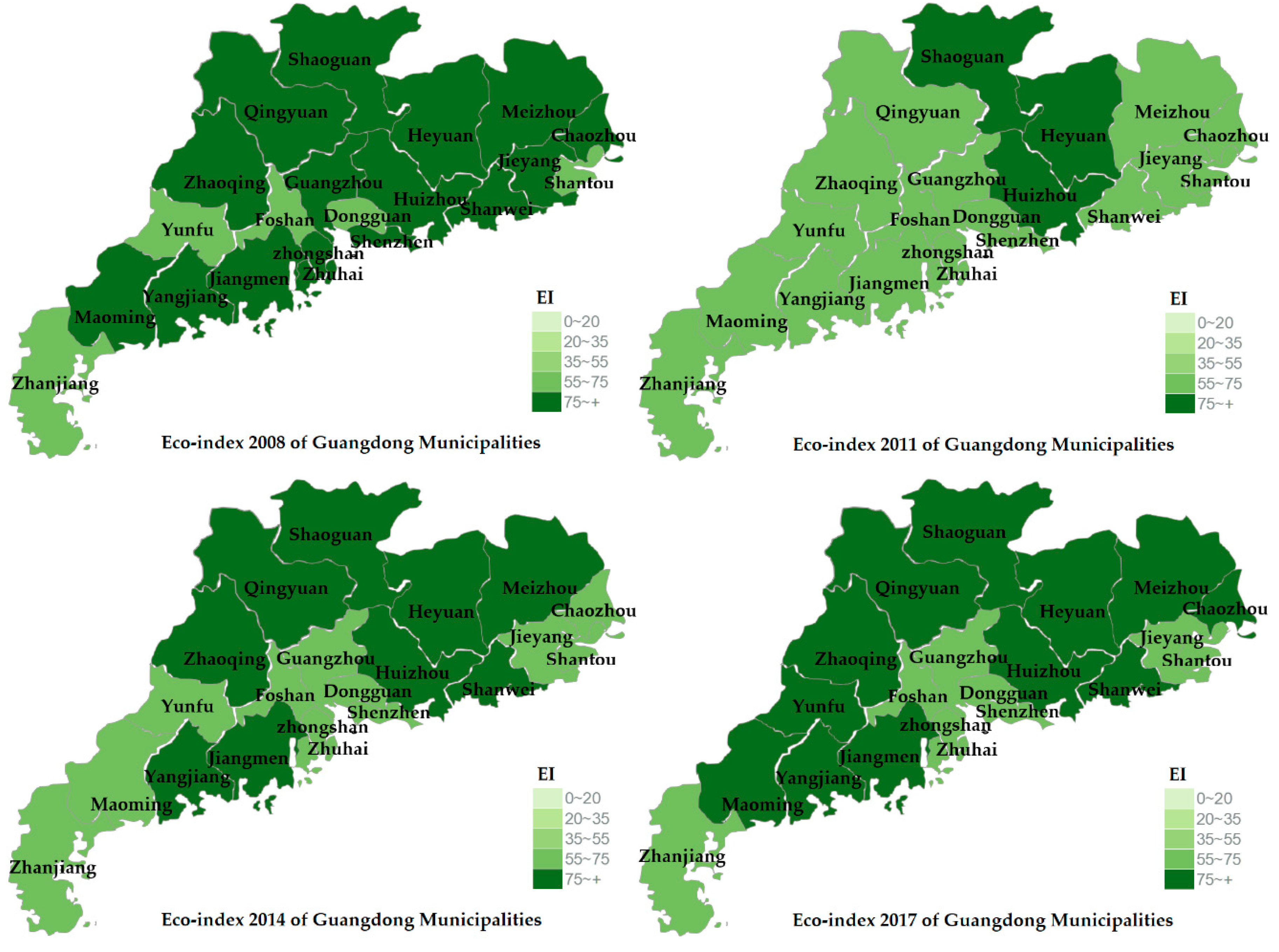
2.1. Ecological Index
2.2. Ecological Sustainable Total Factor Productivity
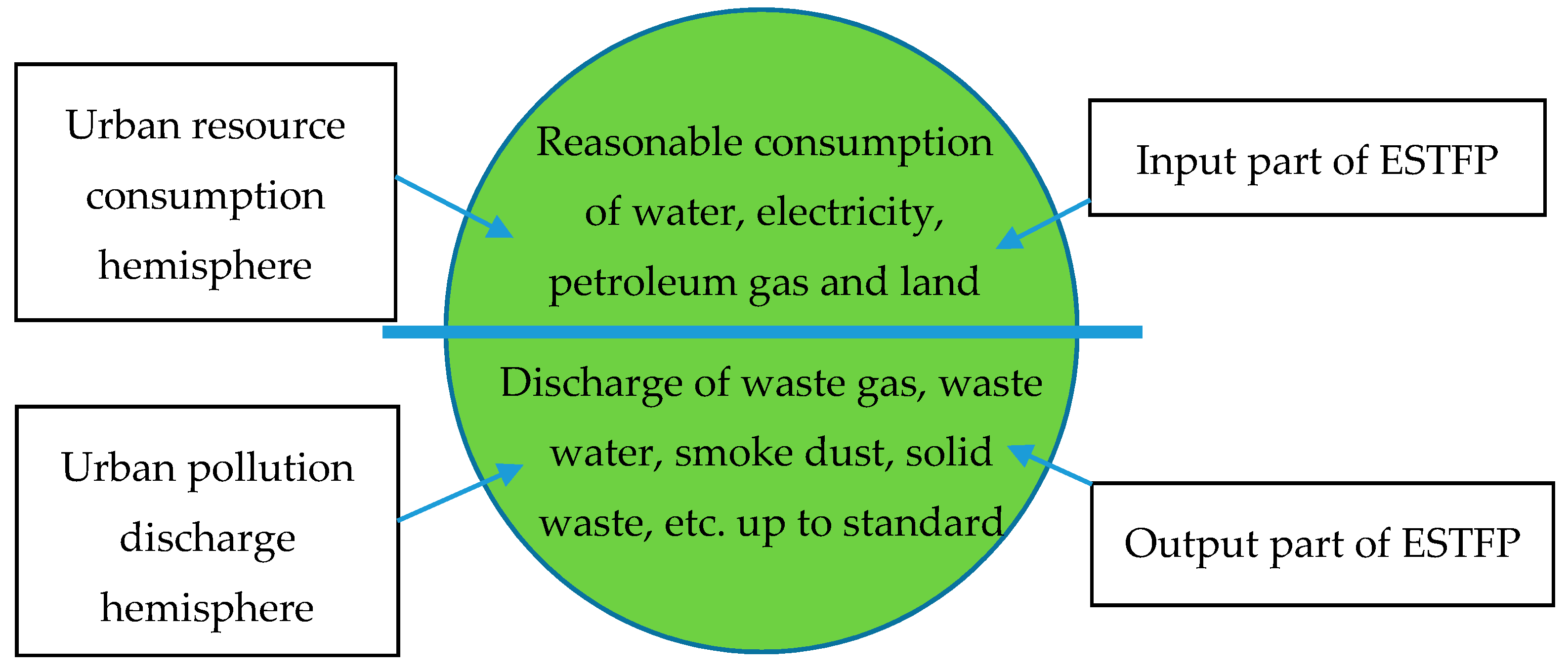
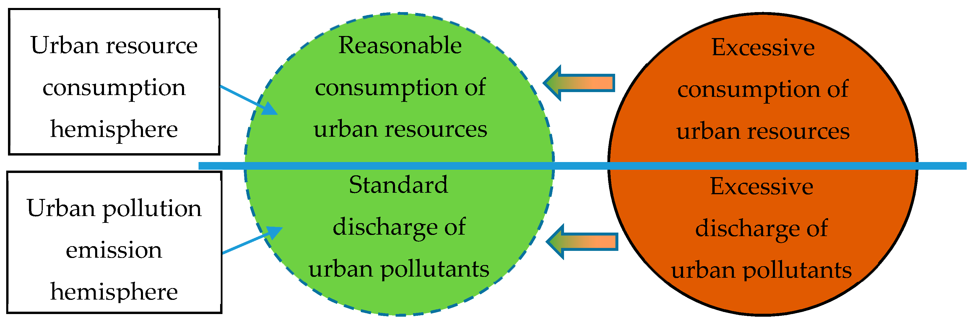
2.2.1. ESTFP Calculation Framework and Urban Ecological Sustainable Hemispheric Theory
2.2.2. Input-Output Variable Selection and Data Sources
2.3. Methods
2.3.1. DEA-Malmquist Index
2.3.2. Panel Data Model
2.4. Research Hypothesis
3. Results and Discussion
3.1. Estimations of ESTFP and Verification of Research Hypotheses
3.1.1. ESTFP Results and Discussion
3.1.2. Research Hypothesis Verification on ESTFP
3.2. Empirical Research Results and Hypothesis Verification of the Relationship between the Ecological Environment and ESTFP
3.2.1. Analysis of Regression Results of the Dynamic Panel Model
3.2.2. Stability Test
3.2.3. Discussion on Regression Results of Panel Data and Verification of Research Hypotheses
4. Conclusions
Author Contributions
Funding
Acknowledgments
Conflicts of Interest
Appendix A
- Biological richness index = (BI + HQ)/2where BI is the biodiversity index and HQ is the habitat quality index.
- Vegetation coverage index= NDVIRegional mean=In the formula, Pi is the average value of the maximum monthly NDVI value of the image elements from May to September, and it is recommended to use the NDVI data of MOD13 with a spatial distribution rate of 250 m. Variable n is the number of regional image elements, and Aveg is the normalization index of the vegetation coverage index with a reference value of 0.0121165124.
- Water network denseness index =where is the normalized index of the river length, and the reference value is 84.3704083981; is the normalized index of the water area, and the reference value is 591.7908642005; is the normalized index of the water resources, and the reference value is 86.3869548281.
- Land stress index = /AreaIn the formula, is the normalized index of the land stress index, and the reference value is 236.0435677948.
- In the formula, is the normalization coefficient of COD, and the reference value is 4.3937397289; is the normalization coefficient of ammonia nitrogen, and the reference value is 40.1764754986; is the normalization coefficient of , and the reference value is 0.0648660287; is the normalization coefficient of smoke (powder) dust, and the reference value is 4.0904459321; is the normalization coefficient of nitrogen oxides, with a reference value of 0.5103049278; is the normalization coefficient of solid waste, and the reference value is 0.0749894283.
- Environmental limit indexThe environmental restriction index is a restrictive index of the ecological environment. It refers to the restriction and adjustment of the ecological environment according to the ecological damage and environmental pollution in the region.
References
- Niemi, G.; McDonald, M. Application of ecological indicators. Annu. Rev. Ecol. Evol. Syst. 2004, 35, 89–111. [Google Scholar] [CrossRef] [Green Version]
- Heink, U.; Kowarik, I. What are indicators? On the definition of indicators in ecology and environmental planning. Ecol. Indic. 2010, 10, 584–593. [Google Scholar] [CrossRef]
- Brazner, J.C.; Danz, N.P.; Niemi, G.J.; Regal, R.R.; Trebitz, A.S.; Howe, R.W.; Reavie, E.D. Evaluation of geographic, geomorphic and human influences on Great Lakes wetland indicators: A multi-assemblage approach. Ecol. Indic. 2007, 7, 610–635. [Google Scholar] [CrossRef]
- Yue, A.; Zhang, Z. Study on the change of ecological status based on EI value. J. Green Sci. Technol. 2018, 14, 182–183. [Google Scholar]
- Zhang, P.; Xu, H.; Du, Q.; Ling, H.; Zhang, P.; Zhao, X. Change of Ecological Conditions in the Mainstream Area of the Tarim River based on RS and GIS. Arid Zone Res. 2017, 2, 416–422. [Google Scholar]
- Li, N.; Tang, Y.; Yang, L.; Xiao, Z.; Chen, Z.; Li, H.; Hu, M. Ecological environment quality of baishui river basin based on remote sensing technology. J. Huazhong Norm. Univ. (Nat. Sci.) 2013, 1, 103–107. [Google Scholar]
- Chung, Y.H.; Färe, R.; Grosskopf, S. Productivity and Undesirable Outputs: A Directional Distance Function Approach. J. Environ. Manag. 1997, 51, 229–240. [Google Scholar] [CrossRef] [Green Version]
- Li, J.; Xu, J. Analysis of the growth trend of green TFP among provinces-Application of a non parametric method. J. Beijing For. Univ. (Soc. Sci.) 2009, 4, 139–146. [Google Scholar]
- Schaltegger, S.; Sturm, A. Ökologische Rationalität: Ansatzpunkte zur Ausgestaltung von ökologieorientierten Managementinstrumenten. Die Unternehm. 1990, 44, 273–290. [Google Scholar]
- Hinterberger, F.; Bamberger, C.; Manstein, P.; Schepelmann, F.; Psangerberg, J. Forestry, Environment and Water; SERI: Vienna, Austria, 2000. [Google Scholar]
- Fet, A. Eco-efficiency Reporting Exemplified by Case Studies. Clean Technol. Environ. Poliy 2003, 5, 232–239. [Google Scholar] [CrossRef] [Green Version]
- Muller, K.; Sturm, A. Standardized Eco-Efficiency Indicators; Ellipson: Basel, Switzerland, 2001. [Google Scholar]
- UNCTAD. A Manual for the Preparers and Users of Eco-Efficiency Indicators; United Nations Publication: New York, NY, USA, 2003. [Google Scholar]
- Seppäläa, J.; Melanen, M.; Mäenpää, I.; Koskela, S.; Tenhunen, J.; Hiltunen, M.R. How Can the Eco-efficiency of a Region be Measured and Monitored? J. Ind. Ecol. 2005, 9, 117–130. [Google Scholar] [CrossRef]
- Zhang, B.B.J.; Fan, Z.; Yuan, Z.; Ge, J. Eco-efficiency Analysis of Industrial System in China: A Data Envelopment Analysis Approach. Ecol. Econ. 2008, 68, 306–316. [Google Scholar] [CrossRef]
- Chen, N.; Xu, L.; Chen, Z. Environmental efficiency analysis of the Yangtze River Economic Zone using super efficiency data envelopment analysis (SEDEA) and tobit models. Energy 2017, 134, 659–671. [Google Scholar] [CrossRef]
- Tugcu, C.T.; Tiwari, A.K. Does renewable and/or non-renewable energy consumption matter for total factor productivity (TFP) growth? Evidence from the BRICS. Renew. Sustain. Energy Rev. 2016, 65, 610–616. [Google Scholar] [CrossRef]
- Li, K.; Lin, B. Economic growth model, structural transformation, and green productivity in China. Appl. Energy 2017, 187, 489–500. [Google Scholar] [CrossRef]
- Shen, N.; Liao, H.L.; Deng, R.M.; Wang, Q.W. Different types of environmental regulations and the heterogeneous influence on the environmental total factor productivity: Empirical analysis of China’s industry. J. Clean. Prod. 2019, 211, 171–184. [Google Scholar] [CrossRef]
- Wen, J.; Wang, H.; Chen, F.; Yu, R. Research on environmental efficiency and TFP of Beijing areas under the constraint of energy-saving and emission reduction. Ecol. Indic. 2018, 84, 235–243. [Google Scholar] [CrossRef]
- Solow, R.M. Technical Change and the Aggregate Production Function. Rev. Econ. Stat. 1957, 39, 312–320. [Google Scholar] [CrossRef] [Green Version]
- Jreisat, A.; Hassan, H.; Shankar, S. Determinants of the Productivity Change for the Banking Sector in Egypt. Glob. Bus. Rev. 2018, 19, 280–296. [Google Scholar] [CrossRef]
- Hu, Z.; Khan, M.S. Why is China Growing So Fast? Int. Monet. Fund Staff Pap. 1997, 44, 1–36. [Google Scholar] [CrossRef] [Green Version]
- Young, A. Gold into Base Metals: Productivity Growth in The People’s Republic of China during the Re- form Period. J. Political Econ. 2003, 111, 1226–1261. [Google Scholar]
- Bosworth, B.; Collins, S.M. Accounting for Growth: Comparing China and India. J. Econ. Perspect. 2008, 22, 45–66. [Google Scholar] [CrossRef] [Green Version]
- Chow, G. Capital Formation and Economic Growth in China. Q. J. Econ. 1993, 108, 809–842. [Google Scholar] [CrossRef]
- Chow, G.; Lin, A.L. Accounting for Economic Growth in Taiwan and Mainland China: A Comparative Analysis. J. Comp. Econ. 2002, 30, 507–530. [Google Scholar] [CrossRef] [Green Version]
- Wang, X.; Fan, G.; Liu, P. Transformation of Growth Pattern and Growth Sustainability in China. Econ. Res. J. 2009, 1, 4–16. [Google Scholar]
- Färe, R.; Grosskopf, S.; Norris, M.; Zhang, Z. Productivity Growth, Technical Progress, and Efficiency Change in Industrialized Countries. Am. Econ. Rev. 1994, 84, 66–83. [Google Scholar]
- Jafri, R.A.; Khan, S.; Shah, M.H.; Baig, N. Total Factor Of Productivity And Its Components: Evidence From Cement - And Energy Sectors Of Pakistan. Risus-J. Innov. Sustain. 2018, 9, 55–73. [Google Scholar] [CrossRef] [Green Version]
- UNDP. China Sustainable Cities Report 2016: Measuring Ecological Input and Human Development; United Nations Development Programme: Beijing, China, 2016. [Google Scholar]
- Zhang, J.; Wu, G.; Zhang, J. The Estimation of China’s provincial capital stock: 1952–2000. Econ. Res. J. 2004, 10, 35–44. [Google Scholar]
- Shi, X.A.; Li, L.S. Green total factor productivity and its decomposition of Chinese manufacturing based on the MML index:2003–2015. J. Clean. Prod. 2019, 222, 998–1008. [Google Scholar] [CrossRef]
- Zhang, J.S.; Tan, W. Study on the green total factor productivity in main cities of China. Zb. Rad. Ekon. Fak. U Rijeci-Proc. Rij. Fac. Econ. 2016, 34, 215–234. [Google Scholar] [CrossRef]
- Malmquist, S. Index numbers and indifference surfaces. Trabajos de Estadistica 1953, 4, 209–242. [Google Scholar] [CrossRef]
- Caves, D.W.; Christensen, L.R.; Diewert, W.E. The economic theory of index numbers and the measurement of input, output, and productivity. Econometrica 1982, 50, 1393–1414. [Google Scholar] [CrossRef]
- Arellano, M.; Bond, S. Some Tests of Specification for Panel Data: Monte Carlo Evidence and anApplication to Employment Equations. Rev. Econ. Stud. 1991, 58, 277–297. [Google Scholar] [CrossRef] [Green Version]
- Arellano, M.; Bover, O. Another Look at the Instrumental Variable Estimation of Error ComponentModels. J. Econom. 1995, 68, 29–51. [Google Scholar] [CrossRef] [Green Version]
- Yu, H.; Liu, Y.; Zhao, J.; Li, G. Urban Total Factor Productivity: Does Urban Spatial Structure Matter in China? Sustainability 2020, 12, 214. [Google Scholar] [CrossRef] [Green Version]
- Managi, S.; Jena, P.R. Environmental productivity and Kuznets curve in India. Ecol. Econ. 2008, 65, 432–440. [Google Scholar] [CrossRef]
- Lusong, Z.; Yali, Z. Effect of Export Technical Sophistication Upgrading on Wage Gap: Evidencefrom Province-level Dynamic Panel Data Model with System GMM Estimation. J. Int. Trade 2014, 11, 61–71. [Google Scholar]
- Binglian, L.; Qingbin, L. The Dynamic Analysis of China’s City TFP: 1990–2006—Based on the Malmquist Index and DEA Model. Nankai Econ. Stud. 2009, 3, 139–152. [Google Scholar]
- Yumin, Y. Calculation and analysis of total factor productivity across the country and provinces. Economist 2002, 3, 115–121. [Google Scholar]
- Porter, M.E.; Linde, C.V.D. Toward a New Conception of the Environment-Competitiveness Relationship. J. Econ. Perspect. 1995, 9, 97–118. [Google Scholar] [CrossRef]
- Wang, B.; Wu, Y.; Yan, P. Environmental Efficiency and Environmental Total Factor Productivity Growth in China’s Regional Economies. Econ. Res. J. 2010, 5, 95–109. [Google Scholar]
- Yang, W.; Yuan, X. An analysis of the impact of foreign trade and FDI on environmental pollution-an analysis of impulse response function based on China’s time series: 1982–2006. World Econ. Study 2008, 62–68, 86. [Google Scholar]
- Su, L.; Liao, Y.; Li, Y. What causes “pollution paradise”: Trade or FDI? -Evidence from provincial panel data in China. Econ. Rev. 2011, 97–104, 116. [Google Scholar]
- Romer, P.M. Endogenous Technological Change. J. Polit. Econ. 1990, 98, 71–102. [Google Scholar] [CrossRef] [Green Version]
- Yue, S.; Liu, C. A Contribution to the Empirics ofTotal Factor Productivity. Econ. Res. J. 2006, 90–96, 127. [Google Scholar] [CrossRef] [Green Version]
- Yu, F.; Xu, W.; Wang, P. Human capital quality, skill premium and total factor productivity-An empirical analysis based on employee matching survey in Chinese Enterprises. J. Zhongnan Univ. Econ. Law 2016, 4, 104–111. [Google Scholar]
- Jinhe, Z.; Yali, W. Estimation of Green Total Factor Productivity and the Influencing Factors—An Empirical Verification Based on Dynamic GMM Method. J. Xinjiang Univ. (Philos. Humanit. Soc. Sci.) 2019, 2, 1–15. [Google Scholar]
- Kim, J.; Park, J. The Role of Total Factor Productivity Growth in Middle-Income Countries. Emerg. Mark. Financ. Trade 2018, 54, 1264–1284. [Google Scholar] [CrossRef]
- Balcerzak, A.P.; Pietrzak, M.B. Dynamic Panel Analysis Of Influence Of Quality Of Human Capital On Total Factor Productivity In Old European Union Countries; Glob. Socio-Econ. Conseq. 2016, 5, 1–13. [Google Scholar]
- Yang, S.; Han, X. Green productivity growth effect of trade liberalization and its constraint mechanism-Threshold regression analysis based on Chinese Provincial Panel Data. Econ. Sci. 2016, 4. [Google Scholar] [CrossRef]


| City | 2008 | 2009 | 2010 | 2011 | 2012 | 2013 | 2014 | 2015 | 2016 | 2017 |
|---|---|---|---|---|---|---|---|---|---|---|
| Guangzhou | 76 | 75 | 63 | 61 | 62 | 63 | 62 | 63 | 64 | 62 |
| Shaoguan | 89 | 87 | 78 | 77 | 79 | 79 | 82 | 83 | 84 | 85 |
| Shenzhen | 83 | 76 | 74 | 73 | 72 | 73 | 65 | 66 | 67 | 69 |
| Zhuhai | 100 | 76 | 75 | 72 | 73 | 73 | 70 | 69 | 69 | 71 |
| Shantou | 73 | 73 | 66 | 66 | 67 | 68 | 66 | 66 | 68 | 67 |
| Foshan | 61 | 60 | 58 | 56 | 58 | 59 | 62 | 63 | 63 | 61 |
| Jiangmen | 86 | 86 | 72 | 69 | 72 | 72 | 75 | 74 | 75 | 77 |
| Zhanjiang | 68 | 69 | 63 | 63 | 64 | 64 | 65 | 64 | 66 | 67 |
| Maoming | 79 | 77 | 68 | 66 | 68 | 70 | 72 | 72 | 75 | 78 |
| Zhaoqing | 85 | 81 | 73 | 72 | 74 | 74 | 80 | 80 | 80 | 82 |
| Huizhou | 89 | 83 | 74 | 75 | 76 | 78 | 81 | 81 | 83 | 81 |
| Meizhou | 84 | 80 | 75 | 73 | 74 | 77 | 79 | 80 | 83 | 84 |
| Shanwei | 90 | 84 | 75 | 74 | 75 | 78 | 77 | 77 | 79 | 80 |
| Heyuan | 90 | 87 | 78 | 76 | 77 | 78 | 80 | 81 | 83 | 83 |
| Yangjiang | 86 | 88 | 76 | 74 | 76 | 76 | 77 | 77 | 78 | 82 |
| Qingyuan | 85 | 82 | 76 | 74 | 76 | 78 | 81 | 82 | 83 | 84 |
| Dongguan | 61 | 61 | 61 | 58 | 60 | 61 | 60 | 60 | 62 | 60 |
| Zhongshan | 85 | 72 | 68 | 65 | 67 | 68 | 67 | 66 | 67 | 64 |
| Chaozhou | 76 | 73 | 68 | 66 | 67 | 69 | 70 | 71 | 74 | 77 |
| Jieyang | 81 | 77 | 70 | 68 | 69 | 72 | 71 | 71 | 74 | 74 |
| Yunfu | 73 | 70 | 67 | 65 | 67 | 67 | 73 | 72 | 74 | 82 |
| mean | 80.95 | 77 | 70.38 | 68.71 | 70.14 | 71.29 | 72.14 | 72.29 | 73.86 | 74.76 |
| Influence Factor | Indicators | Measurement Method | Symbol Anticipation | Data Sources |
|---|---|---|---|---|
| environmental effect | Ecological index (EI) | See Formula (1) | + | Guangdong Statistics Yearbooks |
| Opening to the outside world | Total imports and exports (open) | total imports and exports/GDP | + | |
| human capital | Number of employees in each city at the end of the year (labor) | Original data is not adjusted | + | |
| government intervention | Fiscal expenditure (epd) | Local general public budget expenditure/GDP | + |
| Variables | Mean | SD | Min | Max | N |
|---|---|---|---|---|---|
| lnESTFP | 0.579 | 0.177 | 0.221 | 1.271 | 168 |
| lnEI | 4.285 | 0.097 | 4.043 | 4.489 | 168 |
| lnopen | 0.830 | 0.654 | 0.033 | 2.696 | 168 |
| lnlabor | 0.028 | 0.020 | 0.009 | 0.089 | 168 |
| lnepd | 0.130 | 0.050 | 0.059 | 0.335 | 168 |
| City | ESEC | ESTC | ESPEC | ESSEC | ESTFPC |
|---|---|---|---|---|---|
| Guangzhou | 1 | 1.062 | 1 | 1 | 1.062 |
| Shenzhen | 1 | 0.984 | 1 | 1 | 0.984 |
| Zhuhai | 1 | 0.924 | 1 | 1 | 0.924 |
| Shantou | 0.964 | 0.909 | 0.96 | 1.004 | 0.876 |
| Foshan | 1 | 1.024 | 1 | 1 | 1.023 |
| Shaoguan | 1 | 0.96 | 1 | 1 | 0.96 |
| Heyuan | 0.973 | 0.91 | 0.961 | 1.013 | 0.886 |
| Meizhou | 1 | 0.863 | 1 | 1 | 0.863 |
| Huizhou | 1.007 | 0.985 | 1.009 | 0.998 | 0.992 |
| Shanwei | 1.037 | 1.085 | 1 | 1.037 | 1.125 |
| Dongguan | 1.017 | 0.9 | 1.014 | 1.003 | 0.916 |
| Zhongshan | 0.998 | 0.957 | 1.01 | 0.987 | 0.955 |
| Jiangmen | 0.966 | 0.951 | 0.98 | 0.986 | 0.919 |
| Yangjiang | 1.041 | 0.885 | 1.022 | 1.018 | 0.921 |
| Zhanjiang | 1.049 | 1.027 | 1.055 | 0.994 | 1.077 |
| Maoming | 1 | 0.962 | 1 | 1 | 0.962 |
| Zhaoqing | 1.014 | 0.984 | 1.014 | 1 | 0.998 |
| Qingyuan | 0.967 | 1.035 | 0.975 | 0.992 | 1.001 |
| Chaozhou | 1.012 | 0.83 | 1 | 1.012 | 0.84 |
| Jieyang | 0.96 | 1.06 | 0.95 | 1.01 | 1.018 |
| Yunfu | 1 | 0.918 | 1 | 1 | 0.918 |
| mean | 1 | 0.96 | 0.997 | 1.003 | 0.96 |
| Year | ESTFP Framework | Traditional TFP Framework | ||||||||
|---|---|---|---|---|---|---|---|---|---|---|
| ESEC | ESTC | ESPEC | ESSEC | ESTFPC | EC | TC | PEC | SEC | TFPC | |
| 2008–2009 | 1.039 | 0.933 | 1.021 | 1.017 | 0.969 | 0.998 | 0.859 | 1 | 0.998 | 0.858 |
| 2009–2010 | 1.017 | 0.852 | 1.023 | 0.994 | 0.867 | 0.981 | 0.944 | 0.983 | 0.997 | 0.926 |
| 2010–2011 | 1.029 | 0.896 | 1.016 | 1.013 | 0.921 | 1.01 | 0.959 | 1.003 | 1.007 | 0.968 |
| 2011–2012 | 0.995 | 0.954 | 0.98 | 1.015 | 0.949 | 1.005 | 0.957 | 1.009 | 0.996 | 0.962 |
| 2012–2013 | 0.975 | 0.938 | 0.969 | 1.007 | 0.915 | 1.047 | 0.939 | 1.022 | 1.024 | 0.983 |
| 2013–2014 | 0.978 | 1.016 | 0.987 | 0.991 | 0.994 | 0.975 | 0.992 | 0.996 | 0.979 | 0.968 |
| 2014–2015 | 0.988 | 0.976 | 0.983 | 1.005 | 0.964 | 0.982 | 1.004 | 0.97 | 1.013 | 0.985 |
| 2015–2016 | 0.981 | 1.144 | 1.001 | 0.981 | 1.123 | 0.992 | 0.996 | 0.98 | 1.012 | 0.988 |
| mean | 1 | 0.96 | 0.997 | 1.003 | 0.960 | 0.998 | 0.955 | 0.995 | 1.003 | 0.954 |
| Indicators | (1) | (2) | (3) | (4) |
|---|---|---|---|---|
| LnESTFP | LnESTFP | LnESTFP | LnESTFP | |
| L.LnESTFP | 0.639 *** | 0.656 *** | 0.601 *** | 0.602 *** |
| (28.16) | (26.78) | (23.28) | (20.48) | |
| LnEI | 0.635 *** | 0.655 *** | 0.771 *** | 0.725 *** |
| (6.92) | (8.18) | (12.52) | (9.08) | |
| Lnlabor | −0.660 * | 1.044 *** | 2.193 * | |
| (−1.74) | (3.55) | (1.82) | ||
| Lnopen | −0.020 *** | −0.019 *** | ||
| (−12.58) | (−6.02) | |||
| Lnepd | 0.020 | |||
| (0.33) | ||||
| _cons | −2.528 *** | −2.607 *** | −3.102 *** | −2.934 *** |
| (−6.3) | (−7.29) | (−11.71) | (−9.02) | |
| N | 147 | 147 | 147 | 147 |
| AR(1)-p | 0.0388 | 0.0389 | 0.0355 | 0.0361 |
| AR(2)-p | 0.1364 | 0.1364 | 0.1321 | 0.1319 |
| Sargan-p | 0.4306 | 0.4097 | 0.4479 | 0.4568 |
| Indicators | Random Effect Model | Fixed Effect Model | ||||||
|---|---|---|---|---|---|---|---|---|
| (1) | (2) | (3) | (4) | (1) | (2) | (3) | (4) | |
| LnESTFP | LnESTFP | LnESTFP | LnESTFP | LnESTFP | LnESTFP | LnESTFP | LnESTFP | |
| LnEI | 0.140 (0.84) | 0.204 (1.18) | 0.303 * (1.84) | 0.378 ** (2.32) | 0.237 (1.29) | 0.237 (1.27) | 0.352 ** (1.99) | 0.400 ** (2.31) |
| Lnlabor | 2.138 (1.36) | 4.567 *** (2.76) | 3.887 ** (2.32) | 0.020 (0.01) | 6.507 ** (2.00) | 6.226 * (1.95) | ||
| Lnopen | −0.079 *** | −0.052 *** | −0.085 *** | −0.057 *** | ||||
| (−4.55) | (−2.74) | (−4.51) | (−2.70) | |||||
| Lnepd | −0.884 *** | −0.908 *** | ||||||
| (−2.93) | (−2.77) | |||||||
| _cons | −0.023 | −0.356 | −0.782 | −0.993 | −0.437 | −0.438 | −1.041 | −1.148 |
| (−0.03) | (−0.47) | (−1.09) | (−1.40) | (−0.56) | (−0.54) | (−1.34) | (−1.51) | |
| N | 168 | 168 | 168 | 168 | 168 | 168 | 168 | 168 |
| Within R2 | 0.0113 | 0.0078 | 0.1317 | 0.1747 | 0.0113 | 0.2638 | 0.1335 | 0.1777 |
| Adj R2 | 0.6818 | 0.6796 | 0.7172 | 0.7298 | 0.6818 | 0.6796 | 0.7172 | 0.7298 |
| Indicators | (1) | (2) | (3) | (1) | (2) | (3) | |
|---|---|---|---|---|---|---|---|
| FE | RE | SYSGMM | FE | RE | SYSGMM | ||
| LnEI | 0.400 ** | 0.378 ** | 0.725 *** | L.lnTFP | 0.602 *** | ||
| (2.31) | (2.32) | (9.08) | (20.48) | ||||
| Lnlabor | 6.226 * | 3.887 ** | 2.193 * | _cons | −1.148 | −0.993 | −2.934 *** |
| (1.95) | (2.32) | (1.82) | (−1.51) | (−1.40) | (−9.02) | ||
| Lnopen | −0.057 *** | −0.052 *** | −0.019 *** | Within R2 | 0.1777 | 0.1747 | |
| (−2.70) | (−2.74) | (−6.02) | Adj. R2 | 0.7298 | 0.7298 | ||
| Lnepd | −0.908 *** | −0.884 *** | 0.020 | AR(2)-p | 0.1319 | ||
| (−2.77) | (−2.93) | (0.33) | Sargan-p | 0.4568 |
© 2020 by the authors. Licensee MDPI, Basel, Switzerland. This article is an open access article distributed under the terms and conditions of the Creative Commons Attribution (CC BY) license (http://creativecommons.org/licenses/by/4.0/).
Share and Cite
Yu, H.; Zhao, J. The Impact of Environmental Conditions on Urban Eco-Sustainable Total Factor Productivity: A Case Study of 21 Cities in Guangdong Province, China. Int. J. Environ. Res. Public Health 2020, 17, 1329. https://doi.org/10.3390/ijerph17041329
Yu H, Zhao J. The Impact of Environmental Conditions on Urban Eco-Sustainable Total Factor Productivity: A Case Study of 21 Cities in Guangdong Province, China. International Journal of Environmental Research and Public Health. 2020; 17(4):1329. https://doi.org/10.3390/ijerph17041329
Chicago/Turabian StyleYu, Haidong, and Juanjuan Zhao. 2020. "The Impact of Environmental Conditions on Urban Eco-Sustainable Total Factor Productivity: A Case Study of 21 Cities in Guangdong Province, China" International Journal of Environmental Research and Public Health 17, no. 4: 1329. https://doi.org/10.3390/ijerph17041329