2.1. Numerical Modeling of the New EEG System
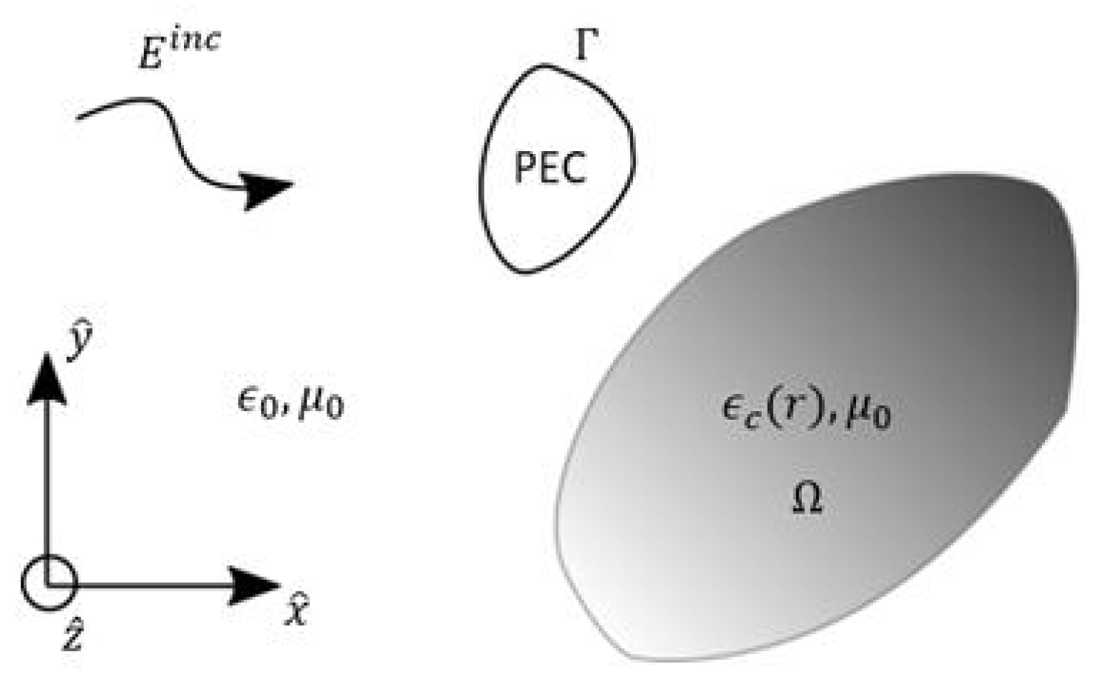
This section briefly describes the numerical solver used to obtain the SAR in a head covered by an EEG net in the presence of an RF source. The requirements for this electromagnetic field solver are to model both the metallic EEG caps and the head, which can be considered as perfectly electric conducting (PEC) surfaces and as an inhomogeneous lossy dielectric material, respectively. The solver chosen is based on the volume–surface integral equation (VSIE) [
11,
12]. It combines a surface integral equation (SIE) to model the PEC objects and a volume integral equation (VIE) to model inhomogeneous bodies. The couplings between the metallic and dielectric objects are included in the VSIE.
Consider a composite scatterer made of a PEC object with boundary
(can be either open or closed) and a linear inhomogeneous dielectric object
illuminated by a time-harmonic incident electromagnetic wave
in a background medium with permittivity
and permeability
, as shown in
Figure 1.
has a complex permittivity
where
(r) is the dielectric permittivity at position
,
is the conductivity, and
is the angular frequency. Using both the volume equivalence principle and the surface equivalence principle [
13], we replace the dielectric bodies by an equivalent volume current density
and the conducting objects by an equivalent surface current density
defined on their surface. The volume current density is defined as
where
i is the imaginary unit,
is the dielectric contrast, and
is the electric flux.
The total field
E can be written as a sum of the incident field and the scattered fields
where
is the field scattered by
and
is the field scattered by
with
G being the 3D Green’s function in vacuum and the constants
and
being the impedance and the wavenumber in vacuum, respectively.
The volume integral equation in
can be expressed as
On a PEC object, the boundary condition requires that the tangential component of the total electric field vanishes. This gives the surface integral equation on
where
is the surface normal vector.
The VSIE is defined by Equations (5) and (6) and is solved for
and
. The next step is to discretize those equations into a matrix system using the method of moments (MoM) [
13]. The volume
is discretized with tetrahedra and the surface
with triangular patches. Note that the triangular patches must coincide with the faces of the tetrahedra at the junctions between
and
. Rao–Wilton–Glisson (RWG) basis functions
[
14] and Schaubert–Wilton–Glisson (SWG) basis functions
[
15] are used to discretize the unknowns
and
, respectively
where
is the number of SWG functions and
is the number of RWG basis functions.
Applying this discretization and testing the equation with both SWG and RWG basis functions, we obtain a block matrix system
In Equation (
9), the diagonal blocks are respectively the standard VIE and SIE and the off-diagonal block represent the coupling between the volume and surface scatterers. The excitation vector is
for the volume part and
for the surface part. The system is solved for the unknown expansion coefficients
and
.
The total electric field
E in
is directly related to
and the SAR within a tissue of the head can be obtained from the average norm of
E in that tissue
where
is the tissue density and
is its conductivity.
2.2. Design of Experiments (DoE)
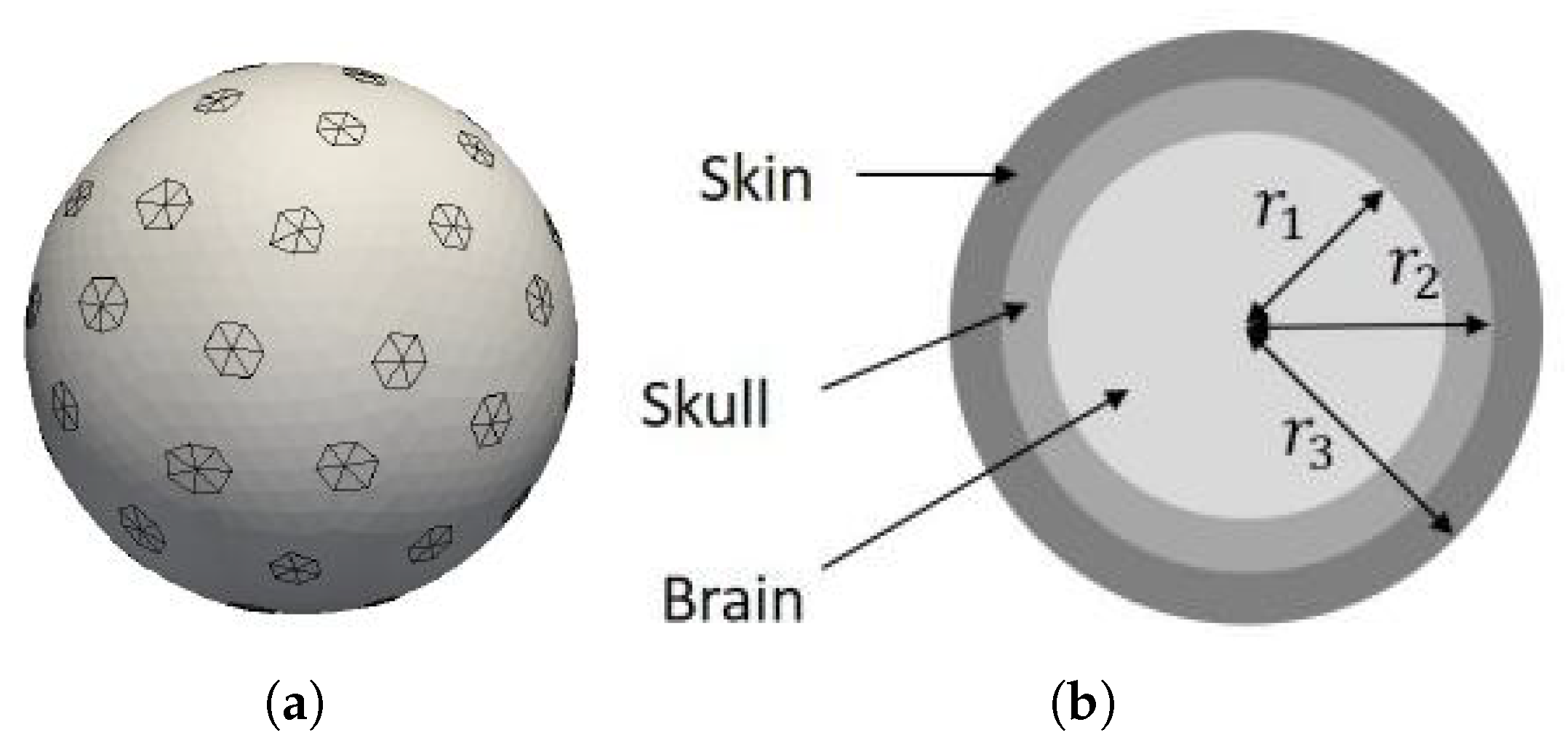
The head model is a three-layer sphere discretized with tetrahedra. The PEC electrodes are formed by the exterior triangles of the tetrahedra pertaining to the boundary of the discretized sphere. The discretized geometry obtained is shown in
Figure 2. In this case, the position of each electrode can be represented by
(
) in a spherical coordinate system, where
r is the radius of the sphere,
is the polar angle,
is the azimuthal angle, and
L is the number of electrodes. The original Cartesian coordinates of the electrodes
are obtained from a toolbox, and are used in the numerical simulations. In the following section, the uncertainties in the positions of the electrodes are modeled in the spherical coordinate system, and the coordinates with uncertainties are required to be transformed into the Cartesian coordinates for numerical simulation.
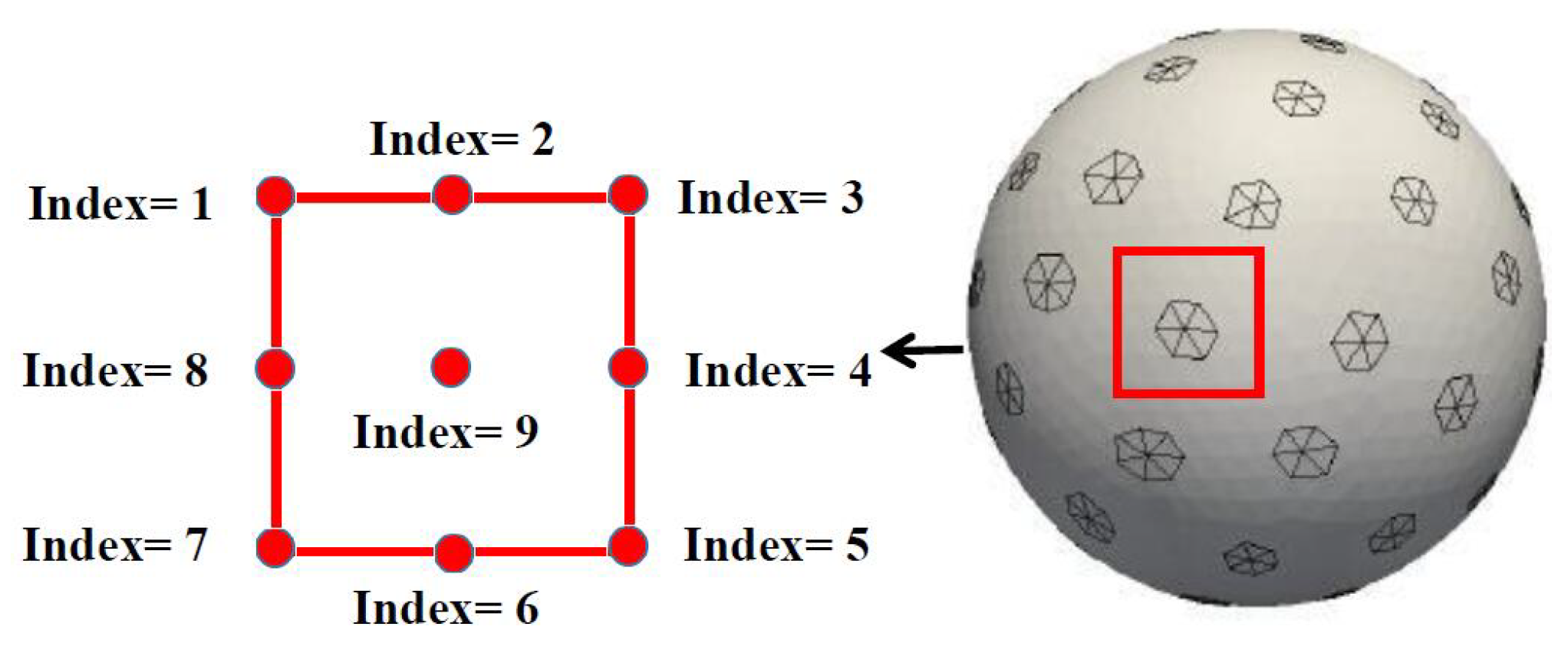
In the spherical coordinate system, the center of each electrode is moved in a square, and the size of the square is controlled by ∆. To simplify the problem, 9 possible positions of the center for each electrode are chosen and represented by 9 indices, which are shown in
Figure 3. The relationship between the indices and the possible positions of the center is provided in
Table 1. When ∆ is determined, the uncertain position of an electrode can be modeled by the nine indices, which makes it a discrete random variable. In the above-mentioned case, the electrodes’ positions are changed independently of one another, and the number of combinations is
.
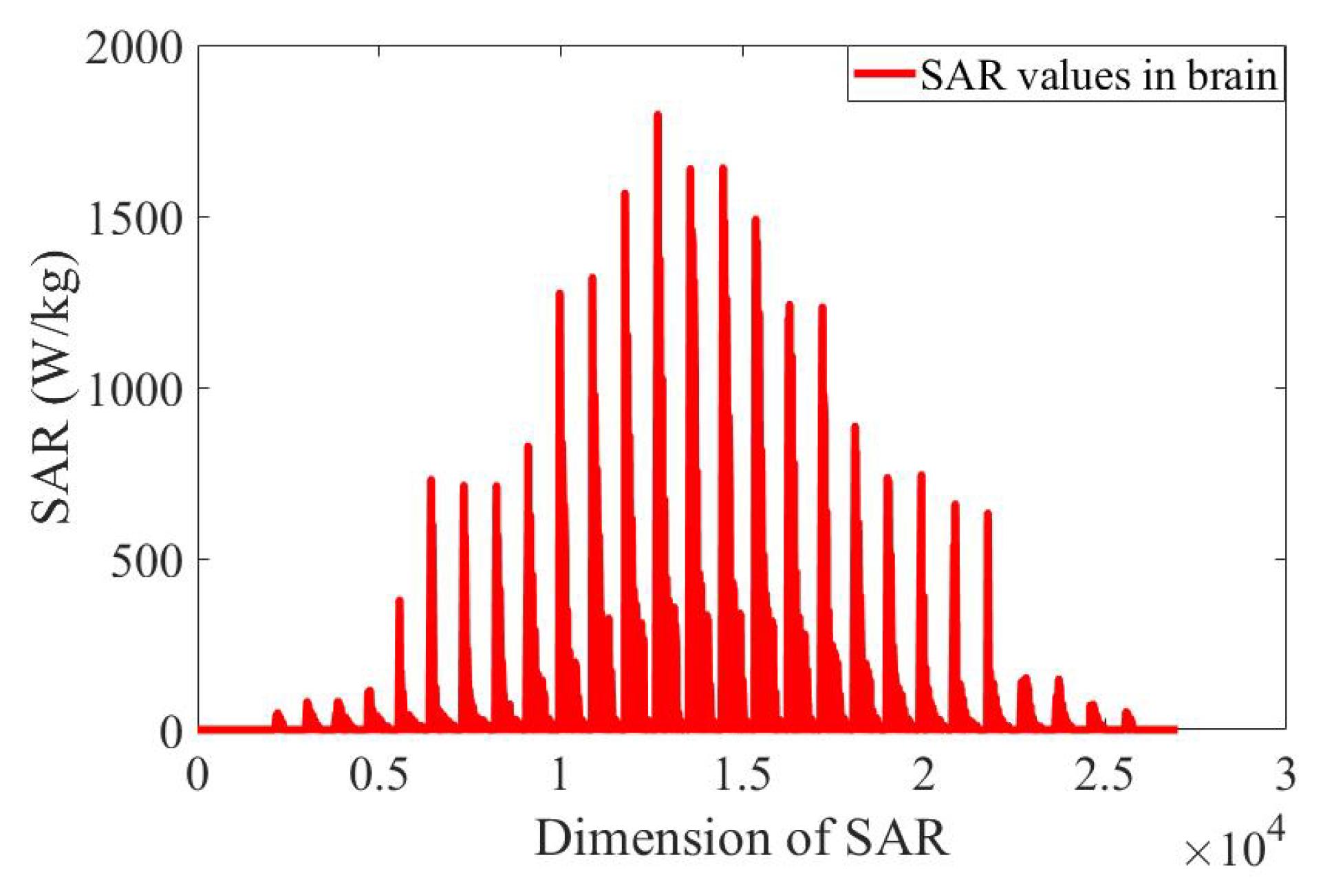
There are three specific issues with this modeling. The first one is that the total CPU time for a single SAR simulation is about 25 h when performed on a computer cluster with 32 cores, which makes impossible the use of MCS directly with the solver. Second, the distance moved by the center of each electrode must be greater than the edge length of the triangle otherwise the algorithm used in the toolbox will arrange the electrode in its original position. This means there is a discrete variation of the uncertain inputs and this variation must be relatively large. Third, the SAR values in brain are high-dimensional data, and there is a small number of high-dimensional SAR values available. To solve the aforementioned problems, an ANN model for UQ is presented in the following section.
2.3. Proposed Surrogate Model for UQ
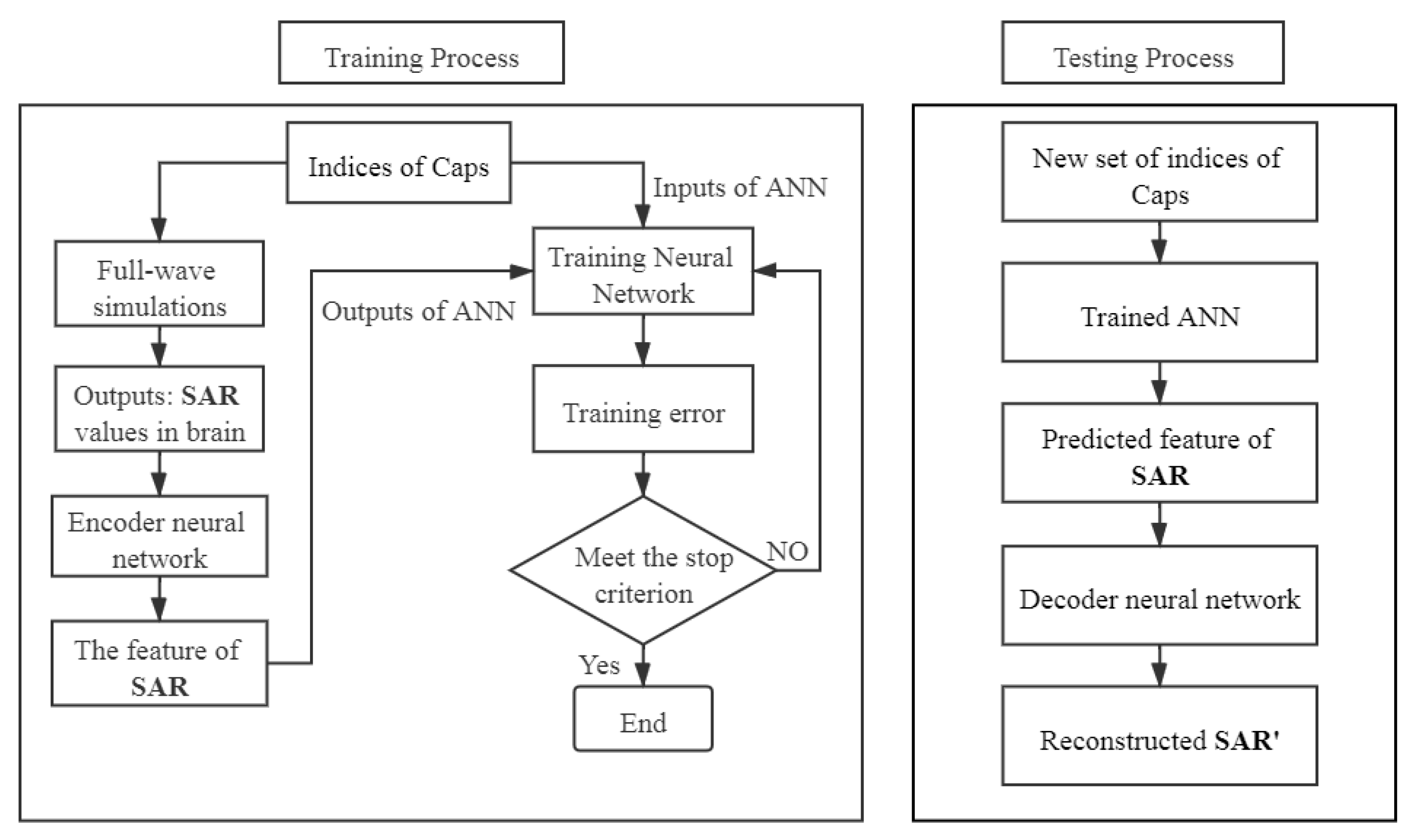
The structure of the new surrogate model is shown in
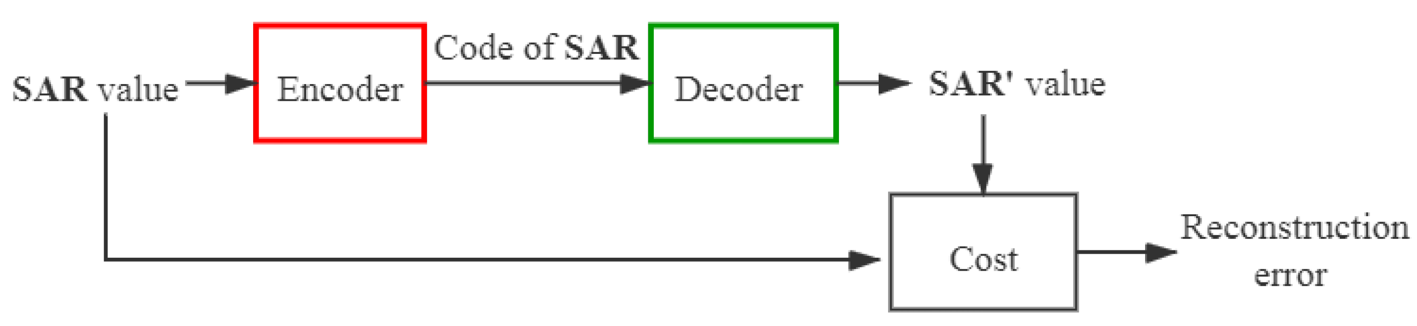
Figure 4. Since the output (SAR values observed in the brain) of the numerical simulation is high-dimensional, it is difficult to handle it with a conventional input-output structure of ANN. Therefore, a pre-trained autoencoder neural network is introduced into the proposed surrogate model for dimensionality reduction to map the high-dimensional outputs to a suitable low-dimensional space, and also for reconstructing the original high-dimensional data.
First of all, an autoencoder neural network is trained. It can be divided into two separate networks: an encoder and a decoder. The structure of an autoencoder neural network is presented in
Figure 5. Given the training data
(
(
) represents a D-dimensional vector
), the encoder transforms the input matrix
into a hidden representation
(
represents a d-dimensional vector
) through activation functions, where
, and
N is the number of input samples for the autoencoder neural network. Then, the matrix
is transformed back to a reconstruction matrix
(
is a D-dimensional vector
) by the decoder.
Subsequently, the proposed ANN is trained. The input samples of the proposed ANN are ( () represents a S-dimensional vector ), which are the uncertain inputs of the EEG numerical simulation, and ( represents a d-dimensional vector ), which are the predicted features of from the encoder neural network, where M is the number of input samples for the proposed ANN.
Finally, in the testing process, the compressed codes can be obtained from the proposed ANN for a new set of uncertain inputs , and then using the decoder, the predicted outputs corresponding to the new set of inputs are obtained. The proposed ANN model can predict the outputs of the numerical simulation very quickly. The statistical quantities of SAR values in brain can be evaluated by running the surrogate model instead of running numerous of numerical simulations.
The hyperparameters of the two ANNs such as the number of hidden layers and units, activation function, learning rate, etc., depending on the data of the problem. In this work, the rectified linear unit (Relu) function [
16] is used as the activation function in both the hidden layers of the autoencoder neural network and the proposed ANN. The Relu function is
and the linear activation function [
17] is used as activation function in the input layer and the output layer of the ANNs. The linear activation function is
where
a is the input to a neuron. The backpropagation algorithm is used to train the two neural networks, and the parameters are optimized through adaptive moment estimation (Adam) [
17]. The mean squared error (MSE) is used for performance evaluation in the ANN
where
and
denote the observed and forecasted values, respectively, of the
rth datum, and
R is the total number of the data.


