3.1. Model for Measuring Biased Technical Change
The DEA method has been widely used to estimate the Shephard output distance function [
41], which can serve as a measure of output technical efficiency [
42] and equals the ratio of actual outputs of a DMU (decision-making unit) to the potentially optimal outputs of DMUs in the production frontier holding inputs constant. The output technical efficiency for DMU “
k” can be obtained by solving the following linear programming problem,
where
is the Shephard output distance function or the output technical efficiency for DMU “
k” among the
R DMUs when constant returns to scale holds.
represents the
N non-negative inputs in period
t, and
represents the
M non-negative outputs produced in period
t.
are the intensity variables in period
t, which are non-negative.
Following Färe et al. [
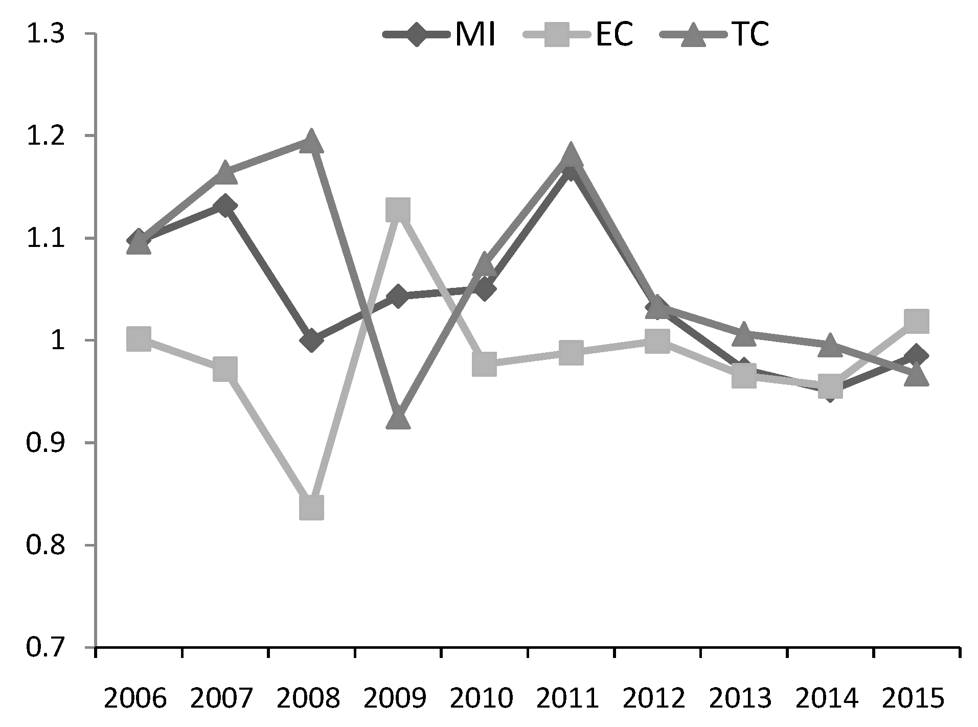
25], the output technical efficiency growth can be estimated using the output-based Malmquist index (hereafter MI) as shown in Formula (2). This index can be decomposed into two indices measuring efficiency change (hereafter EC) and technical change (hereafter TC). The efficiency change measures the ‘‘catching up” to the production frontier, reflecting the change of organizational management ability, while the technical change measures the shift of the production frontier from one period to another, reflecting the level of technical progress. As the product of EC and TC, the MI index reflects the overall technical efficiency growth of each DMU. According to Färe et al. [
25], the output-based Malmquist index and the decomposition indices take the following form
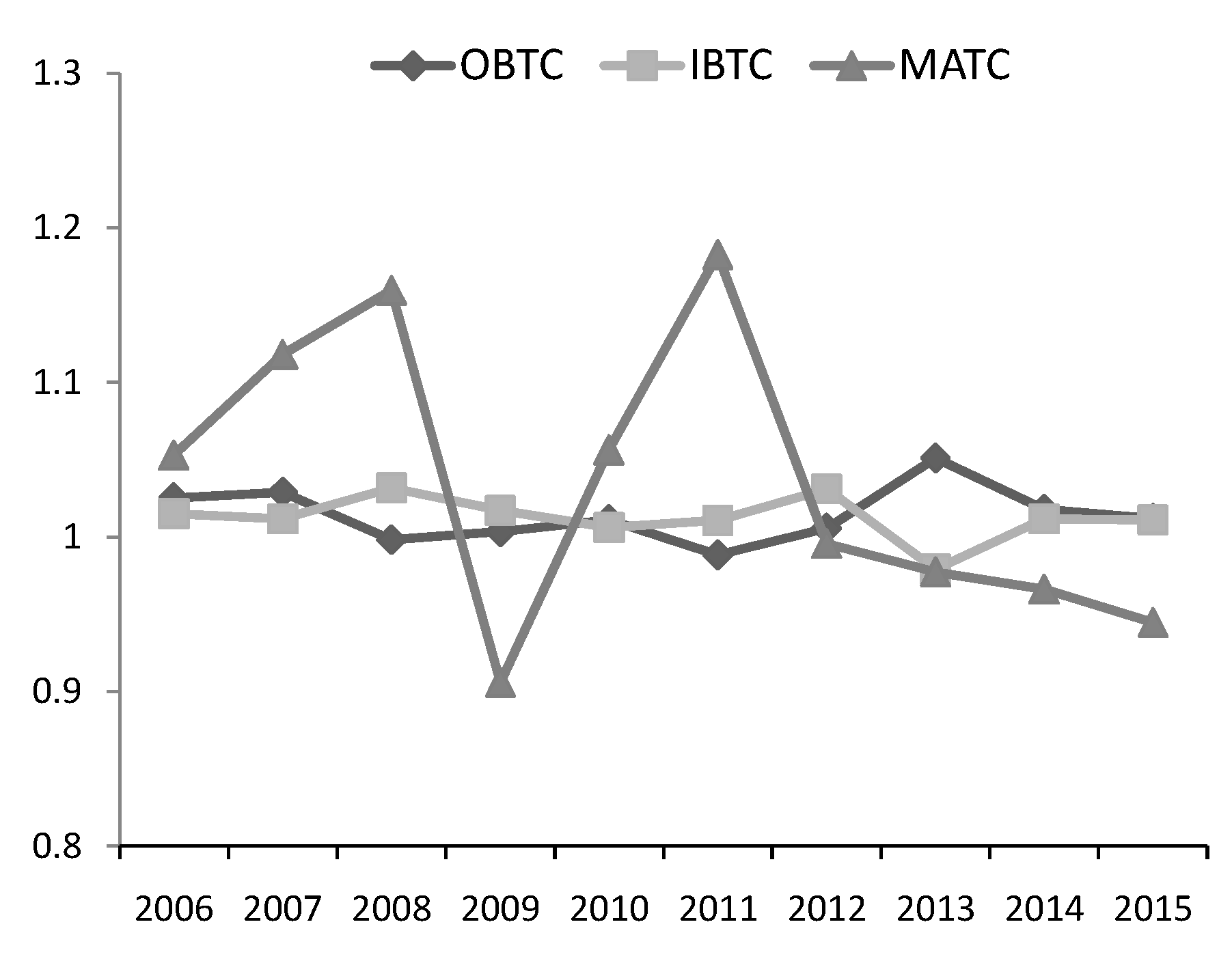
Furthermore, Färe and Grosskopf [
32] decomposed the TC index into three separate indices including output-biased technical change (OBTC), input-biased technical change (IBTC) and the magnitude of technical change (MATC). These indices can disclose the tilted effects of the production frontier, measuring the contribution of three types of technical change including output-biased technical change, input-biased technical change and neutral technical change to the overall technical change and productivity growth. The three indices take the following forms:
If OBTC > 1, it means that the bias of output promotes technical progress and productivity growth, otherwise it leads to technical regress and productivity decline. OBTC = 1 means that there is no bias among outputs. If IBTC < 1, it indicates that the bias of input promotes technical progress and productivity growth, otherwise it leads to technical regress and productivity decline. IBTC = 1 indicates that there is no bias among inputs; MATC represents the magnitude of Hicks’ neutral technical progress. MATC > 1 means that the neutral technology promotes technical progress, and vice versa leads to technical regress. The Meanings of OBTC, IBTC and MATC are shown in
Table 1.
However, the indicator of OBTC or IBTC can only disclose whether the outputs or inputs are biased and whether the bias promotes technical progress, it can not directly indicate which output or input is biased. Weber and Domazlicky [
33] and Barros and Weber [
35] illustrate how to identify the directions of input bias and output bias in the biased technical change. In their analysis, the identifying criteria for biased technical change are on the ground of the input-based Malmquist productivity index. Färe et al. [
36] demonstrate the criteria for identifying the direction of input bias in the biased technical change with the output-based Malmquist productivity index. We illustrate how to identify the directions of both the output and input bias in the biased technical change with the output-based Malmquist productivity index, then employing the identifying criteria to analyze the industrial green biased technical change in terms of water resources in China’s Yangtze River Economic Belt. The identifying criteria are shown in
Table 2, which is derived from
Figure 3 and
Figure 4.
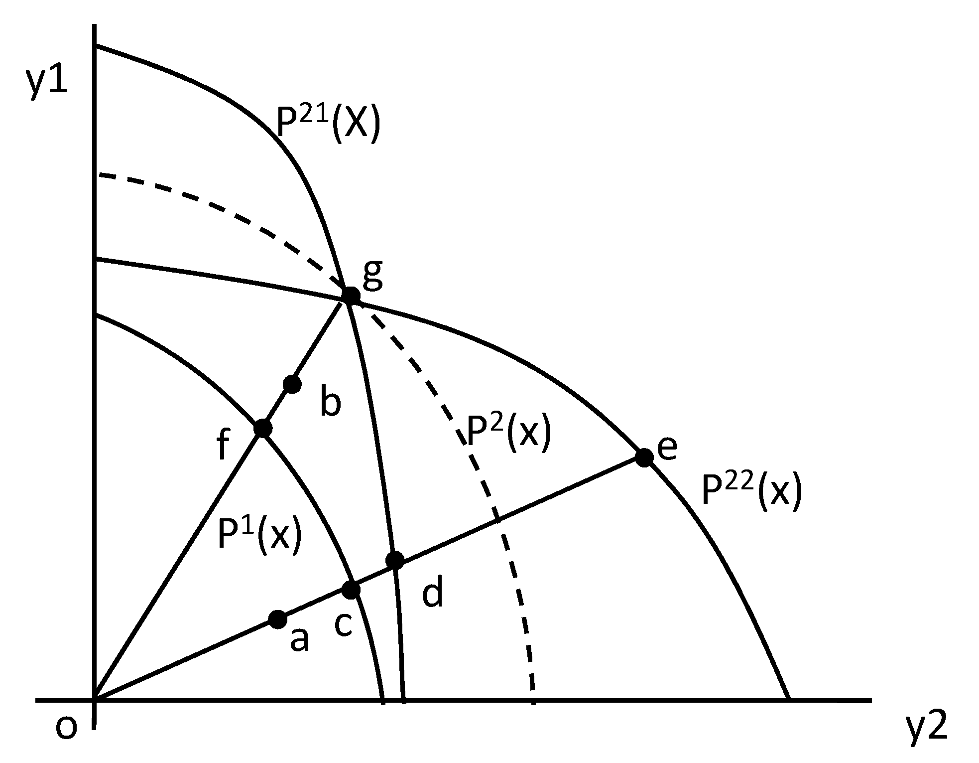
Figure 3 illustrates the construction of the output-biased technical change index. The production possibility frontier in period t is represented as P
t(x), the inputs x can produce the outputs y, which include y
1 and y
2. We assumed there exists technical progress from period 1 to period 2. Technical progress is Hicks’ neutral if the MRT
y2y1 (marginal rate of transformation) between two outputs of y
1 and y
2 remains constant. In this scenario, the production possibility frontier P
1(x) in period 1 will move in parallel to P
2(x) in period 2. If the technical progress leads to an output bias, the production possibility frontier will tilt when moving from period 1 to period 2. According to Weber and Domazlicky [
33] and Barros and Weber [
35], if the MRT
y2y1 increases, the production possibility frontier in period 2 will be P
21(x), indicating that the technical progress is biased towards y
1, or y
1-producing biased technical change. Otherwise, if MRT
y2y1 decreases, the production possibility frontier in period 2 will be P
22(x), indicating that the technical progress is biased towards y
2, or y
2-producing biased technical change. Now suppose that the output mix (y
1, y
2)
t for a DMU is at point “a” in period 1 and at point “b” in period 2, that means
, and suppose that the production possibility frontier is P
1(x) in period 1 and P
21(x) in period 2 which means there exists y
1-producing biased technical change. In this situation, the Shephard output distance function in period 1 is
, and in period 2 is
. The two inter-period input distance functions are calculated as
and
, then according to the Formula (3), the OBTC index of DMU can be calculated as
, so given that
and
, the technical change is biased towards y
1. This is in the first situation. In the second situation, suppose that the outputs mix (y
1, y
2)
t for the DMU in each period and the production possibility frontier P
1(x) in period 1 stay the same as the first situation, but the production possibility frontier in period 2 shifts to P
22(x), which means there exists y
2-producing biased technical change. In this situation, the OBTC index of DMU can be calculated as
, so given that
and
, the technical change is biased towards y
2. In the third situation, if the production possibility frontier is P
2 (x) in period 2, then the
, so given that
, technical change is neutral. The identifying criteria for output bias above are based on
, or the output y
1 is increasing compared to y
2 with time, which means the position of axis “ob” in period 2 is above the position of axis “oa” in period 1 as displayed in
Figure 3. Oppositely, if
, the position of axis “ob” in period 2 would be underneath the position of axis “oa” in period 1. By exchanging the angle of axis “oa” and axis “ob” in
Figure 3, it is not difficult to work out the identifying criteria on the condition of
, which are opposite to those on the condition of
. All the possible identifying criteria for the output-biased technical change are summarized in the left part of
Table 2.
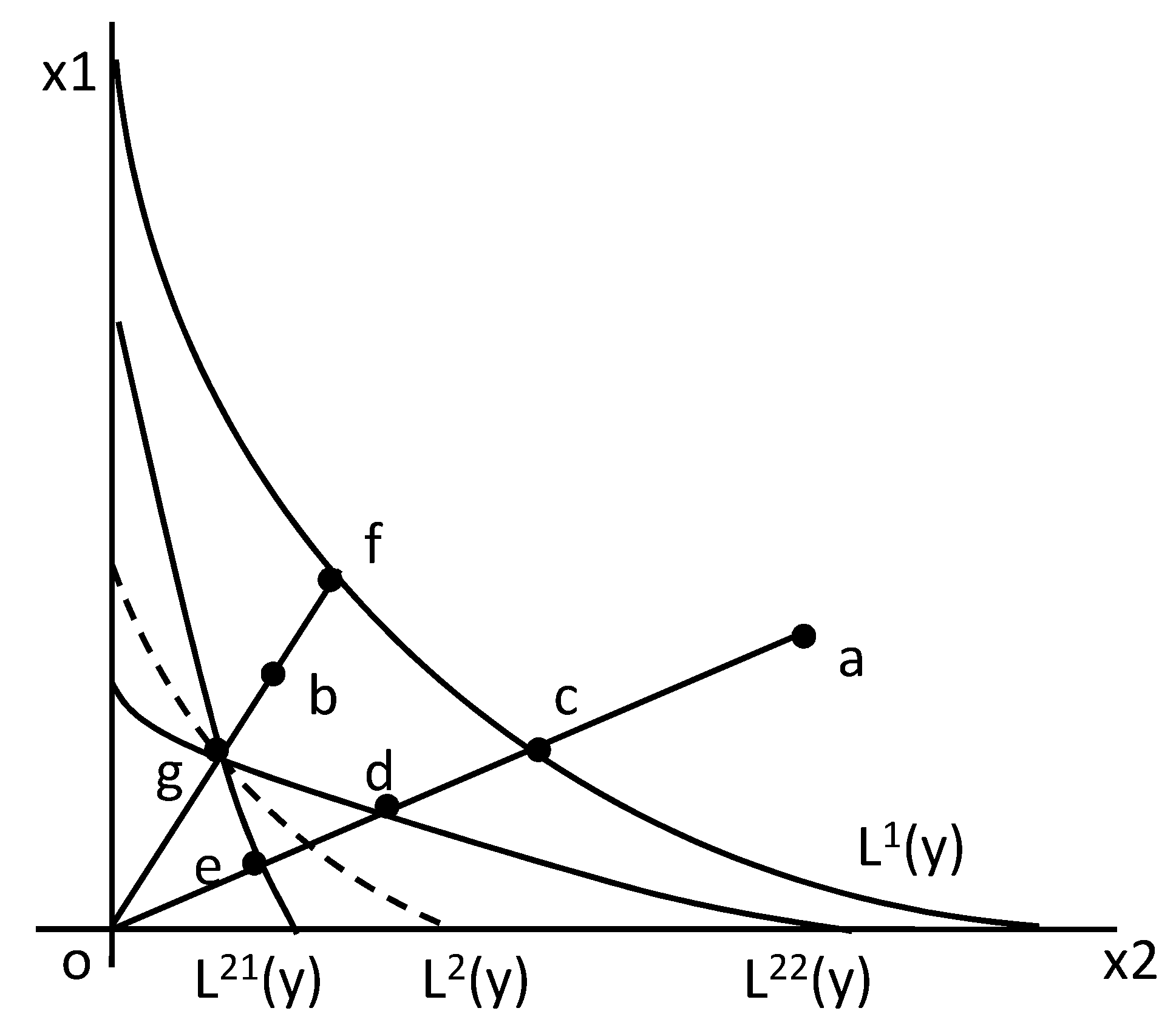
To investigate the input-biased technical change displayed in
Figure 4, we rewrote the IBTC index in Formula (3) by the Shephard input distance function. Under the condition of constant returns to scale, the Shephard input distance function equals the reciprocal of the Shephard output distance function [
43]. That is,
. Therefore, given constant returns to scale we can rewrite the IBTC index in Formula (3) as
Figure 4 illustrates the construction of input-biased technical change index. The isoquant curve in period t is represented as L
t(y), the inputs x can produce the outputs y. There are two kinds of inputs including x
1 and
x2. We assumed there exists technical progress from period 1 to period 2. If the technical progress is Hicks’ neutral, or the MRS
x2x1 (marginal rate of substitution) remains constant, the isoquant curve L
1(y) in period 1 will move in parallel to L
2(y) in period 2. If the technical progress leads to input bias, the isoquant curve will tilt when moving from period 1 to period 2. If the MRS
x2x1 increases, the isoquant curve in period 2 will be L
21(y), indicating that the technical progress is biased towards saving
x1, or
x2-using biased technical change. Otherwise, if MRS
x2x1 decreases, the isoquant curve in period 2 will be L
22(y), indicating that the technical progress is biased towards saving x
2, or x
1-using biased technical change. Now suppose that the input mix (x
1,
x2)
t for a DMU is at point “a” in period 1 and at point “b” in period 2, which means
, and suppose that the isoquant curve is L
1(y) in period 1 and L
21(y) in period 2, which mean there exists x
2-using or x
1-saving biased technical change. In this situation, The Shephard input distance function in period 1 is
, and in period 2 is
. The two inter-period input distance functions are calculated as
and
. Then according to the Formula (4), the IBTC of the DMU can be calculated as
. So, given that
and
, the technical change is biased towards x
2-using or x
1-saving. This is in the first situation. In the second situation, suppose that the input mix (x
1, x
2)
t for the DMU in each period and the isoquant curve L
1(y) in period 1 stay the same as the first situation, but the isoquant curve in period 2 shifts to L
22(y), which means there exists x
1-using or x
2-saving biased technical change. In this situation, IBTC of the DMU can be calculated as
, so given that
and
, the technical change is biased towards x
1-using or x
2-saving. In the third situation, if the isoquant curve is L
2 (y) in period 2, then
, so give that
, the technical change is neutral. The identifying criteria above for input bias are based on the condition of
, or the input ratio of x
1 and x
2 is increasing with time, which means the position of axis “ob” in period 2 is above the position of axis “oa” in period 1 as displayed in
Figure 4. Oppositely, if
, the position of axis “ob” in period 2 would be underneath the position of “oa” in period 1. By exchanging the angle of axis “oa” and axis “ob” in
Figure 4, it is not difficult to work out the identifying criteria for input bias on the condition of
, which are opposite to those on the condition of
. All the possible identifying criteria for the input-biased technical change are summarized in the right part of
Table 2.
It should be noted that the identifying criteria for biased technical change in
Table 2 are derived from the output-based Malmquist productivity index as by Fare et al. [
36]. The results are a little different to those of Weber and Domazlicky [
33] and Barros and Weber [
35]. The criteria for biased technical change constructed by Weber and Domazlicky [
33] and Barros and Weber [
35] are derived from the input-based Malmquist productivity index, which is the reciprocal of output-based Malmquist productivity index given constant returns to scale. Therefore, in our research, OBTC > 1 or IBTC >1 indicates a biased technical progress rather than biased technical regress as in their research. After controlling this difference, the identifying criteria of
Table 2 is substantially consistent with those of Weber and Domazlicky [
33] and Barros and Weber [
35].
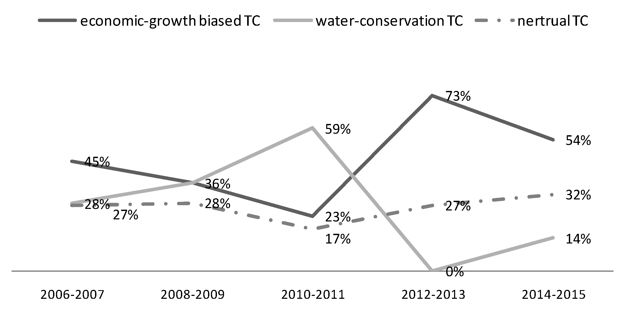
The economic meaning for the identifying criteria of output-biased technical change in
Table 2 can be well explained. Under the y
1-producing biased technical change mode, only if the growth rate of output y
1 from period 1 to period 2 is higher than that of output y
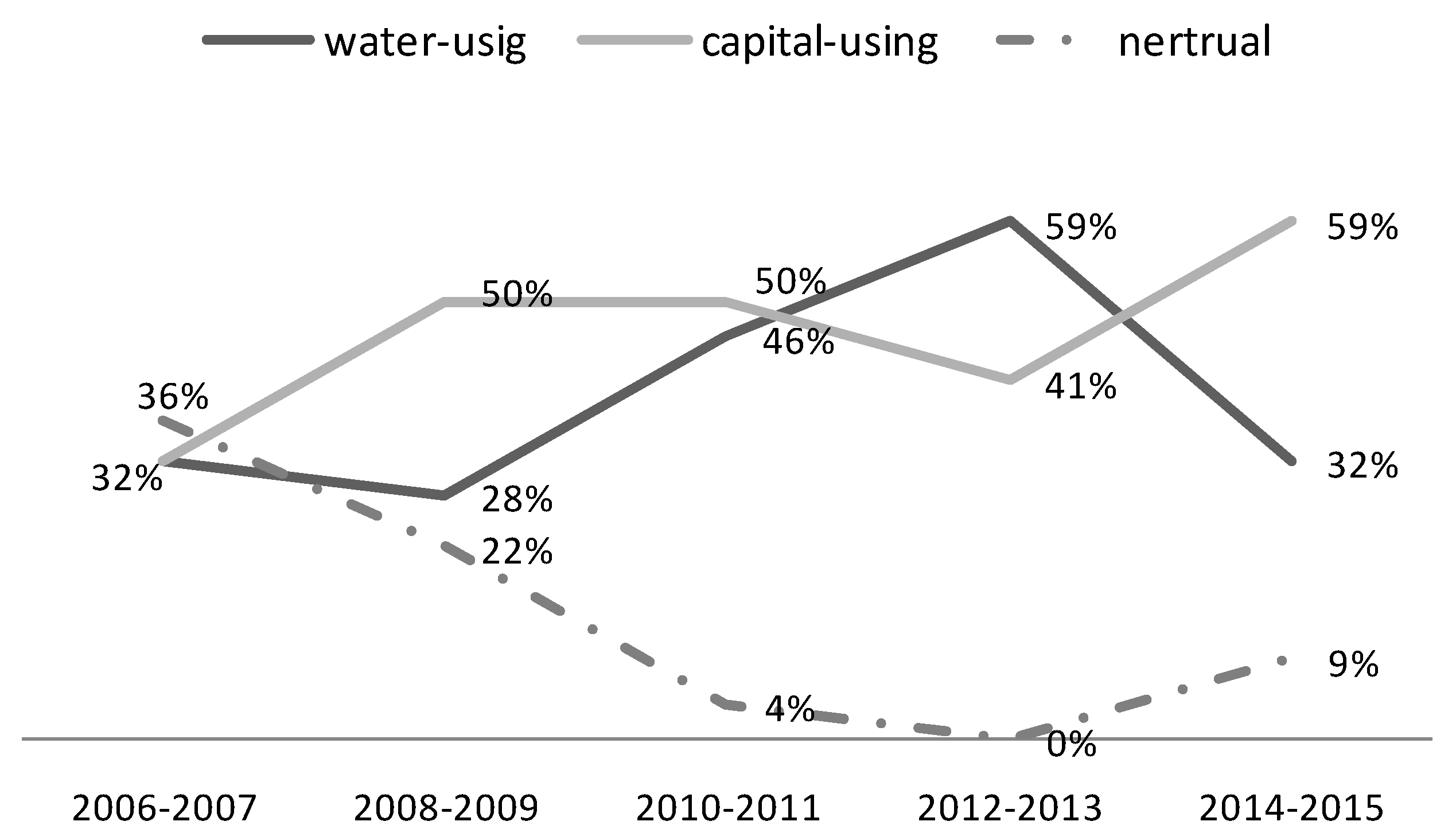
2 can the productivity be promoted by the output-biased technical change (OBTC > 1), otherwise, the productivity will decrease (OBTC < 1). In short, the structure of output mix needs to match the inner request of the output-biased technical change in order to promote the productivity. The economic meaning is similar for the identifying criteria of input-biased technical change. Under the x
1-using or
x2-saving technical change mode, only if the saving speed of input x
2 from period 1 to period 2 is faster than that of input x
1 can the productivity be promoted by the input-biased technical change (IBTC > 1), otherwise the productivity will decrease (IBTC < 1). In short, the structure of input mix needs to match the inner request of the input-biased technical change in order to promote the productivity.
3.2. Indicators and Data
In our research, two output indicators were considered including the industrial added value and COD clean index.
Industrial added value: The industrial added value represents the economic output of the industrial economic development. It is measured by the added value of industrial enterprises above the designated size in each provincial region across China. It is deflated by the deflator of the industrial producer price index and denoted at the price of 2005.
COD clean index: COD clean index is constructed to measure water conservation performance, which is related to the COD emission (chemical oxygen demand) among industrial sewage in provincial regions across China. Since COD emission is an undesirable or negative output, it is necessary to transform the negative index to a positive index in order to use the Shephard radial distance function and the identifying criteria of biased technical change in
Table 2, which is derived on the assumption of Shephard radial distance function. One main method for transforming a negative indicator to a positive indicator is to transform the negative indicator to the form of additive inverses (-y), and add to the additive inverses a sufficient large positive constant c, then construct the transformed positive indictor y’ by y’= −y + c [
44,
45]. The advantage of this transformation method is that it does not change the internal linear structure of the original data. In order to ensure that y’ is positive, we let c = y
max + y
min, where y represents the COD emission of each DMU. With y’ = −y + c, the maximum value of original COD emission is reversed to the minimum value, and the original minimum is reversed to the maximum. After that, the COD clean index is constructed by (y’/y’
min) × 100. The COD clean index is the desirable or positive output index. The larger the COD clean index, the cleaner the industrial sewage.
There are three input indicators, including capital stock, labor and water consumption.
Capital stock: Capital stock is measured by the stock of physical assets investment of industrial enterprises above the designated size in provincial regions across China, calculated by the perpetual inventory method [
46] as
, where
Kit represents capital stock of region
i in period
t,
Iit represents capital flow of region
i in period
t,
represents the economic depreciation rate. The initial capital stock in 2005 is presented by the net value of physical assets in 2005. As to the economic depreciation rate
, we assumed a value of 11.6%, which is estimated by Shan et al. [
47] and has been widely adopted in estimating the capital stock in China. The capital stock is deflated by the deflator of the capital investment price index at the price of 2005.
Labor: Labor represents the input of human resources in industrial production. It is represented by the annual average number of employees in industrial enterprises above designated size at provincial level across China.
Water consumption: Water consumption represents the input of water in industrial production. It is measured by the industrial water consumption of industrial enterprises above the designated size at the provincial level across China.
The data for the industrial index, such as the industrial added value, physical assets investment and industrial labor are extracted from China Industry Statistical Yearbook from 2005 to 2015 and the related provincial statistical yearbooks in China. The data for environmental index, such as the water consumption and the COD emission among industrial sewage are taken from China Environmental Statistical Yearbook from 2005 to 2015. The price index is from the China Statistical Yearbook from 2005 to 2015.


