Article

Comparison of Random Forest and Gradient Boosting Machine Models for Predicting Demolition Waste Based on Small Datasets and Categorical Variables

1
Department of Architectural Engineering, Dankook University, Yongin 16890, Korea
2
Department of Safety Engineering, Dongguk University—Gyeongju, Gyeongju 38066, Korea
*
Author to whom correspondence should be addressed.
Int. J. Environ. Res. Public Health 2021, 18(16), 8530; https://doi.org/10.3390/ijerph18168530
Submission received: 23 July 2021 / Revised: 7 August 2021 / Accepted: 8 August 2021 / Published: 12 August 2021

Abstract

:
Construction and demolition waste (DW) generation information has been recognized as a tool for providing useful information for waste management. Recently, numerous researchers have actively utilized artificial intelligence technology to establish accurate waste generation information. This study investigated the development of machine learning predictive models that can achieve predictive performance on small datasets composed of categorical variables. To this end, the random forest (RF) and gradient boosting machine (GBM) algorithms were adopted. To develop the models, 690 building datasets were established using data preprocessing and standardization. Hyperparameter tuning was performed to develop the RF and GBM models. The model performances were evaluated using the leave-one-out cross-validation technique. The study demonstrated that, for small datasets comprising mainly categorical variables, the bagging technique (RF) predictions were more stable and accurate than those of the boosting technique (GBM). However, GBM models demonstrated excellent predictive performance in some DW predictive models. Furthermore, the RF and GBM predictive models demonstrated significantly differing performance across different types of DW. Certain RF and GBM models demonstrated relatively low predictive performance. However, the remaining predictive models all demonstrated excellent predictive performance at R2 values > 0.6, and R values > 0.8. Such differences are mainly because of the characteristics of features applied to model development; we expect the application of additional features to improve the performance of the predictive models. The 11 DW predictive models developed in this study will be useful for establishing detailed DW management strategies.

1. Introduction

Waste management has become a critical issue due to rapid urban growth [1,2]. According to recent statistics, 2.01 billion tons of municipal solid waste (MSW) was generated in 2016; reports also predict that 3.40 billion tons of waste will be generated annually by 2050 [3]. In particular, construction and demolition (C&D) waste generation is steadily increasing [4,5,6], and 70–90% of C&D waste generation can be attributed to demolition activities [7,8]. For example, construction activities are responsible for 90% of the C&D waste generation in the United States; moreover, such activities account for 74% of the C&D waste generation in China [6,7,8]. C&D waste is mainly generated from such activities as construction, demolition, and refurbishment, which are detrimental to the environment because they generate considerable quantities of waste and greenhouse gases [9]. Therefore, systems or solutions for effectively and appropriately managing C&D waste are necessary for sustainable growth and development in the construction industry.
A key requirement for sustainable growth in C&D-related industries is to achieve the maximum economic and environmental values expected during building demolition [10]. To this end, accurate information on the amount of waste generation is necessary, as basic data for predicting the bulk of waste, the economic scale, and the environmental impact [6,11]. Therefore, information on the amount of C&D waste generation is perceived to be useful in informing the management of waste for relevant industry personnel (clients, architects, engineers, contractors, planners, etc.) [12].
Predicting C&D waste is a difficult task because it depends on the technical, cultural, and geometric variables of buildings. ML can be useful for explaining or understanding these variables by combining them; as such, its use in the construction industry has continued to increase [13]. Therefore, recently, numerous researchers have used artificial intelligence (AI) technology to establish accurate waste generation information; the unique characteristics of AI algorithms (data input, learning, and prediction) are considered state-of-the-art models for reliable waste generation prediction [14]. Various AI algorithms—including artificial neural networks (ANN), adaptive neuro-fuzzy inference systems (ANFIS), support vector machines (SVM), linear regression analysis (LR), and decision trees (DT)—have been applied as machine learning (ML) methods for the prediction of MSW and C&D waste generation. However, application of such AI systems requires big data, and insufficient data can be a major obstacle to the predictive performance of AI models [15]. Most existing studies, using such methods as ANN [10,16,17], SVM [16,18,19], and LR [16,20,21,22], are based on big data consisting of continuous variables; in other data environments (categorical variables, small datasets, etc.), the waste prediction performance seen in existing studies cannot be guaranteed [23], because predictive models using ML algorithms based on small datasets cannot be free of statistical bias [24] and high variance [25]. To overcome this limitation of applying AI systems, predictive models must be developed by applying ML algorithms suitable for small datasets composed of categorical variables. A recent study [26] demonstrated that DT-based algorithms exhibit excellent predictive performance for small datasets composed of categorical variables. Such results are expected to help DT-based ML algorithms improve the predictive performance of models for small datasets composed of categorical variables.
This study investigated the performance of predictive models of demolition waste (DW) generation by applying representative DT-based ML algorithms (RF and GBM) as a method to improve the predictive performance of AI models for small datasets composed of categorical variables. To this end, this study (1) built a dataset of information on the amount of generation of 10 types of DW, including the structure, region, purpose of use, wall materials, roof materials, and area variables. (2) To improve the performance of the predictive models, preprocessing was performed by eliminating outliers and normalizing the raw data. (3) Hyperparameters for each algorithm were tuned, and based on (1) and (2), GBM (boosting technique) and RF (bagging technique) algorithms—representative ensemble models based on DT—were applied to derive 10 types of waste generation models and one predictive model for total waste generation, covering all waste types. (4) Considering the characteristics of the data, leave-one-out cross-validation (LOOCV) was applied to verify and evaluate the predictive models. The performance of the models was evaluated using Pearson’s correlation coefficient (R), root mean square error (RMSE), coefficient of determination (R2), and mean absolute error (MAE) metrics. (5) Finally, the ensemble technique suitable for small datasets composed mainly of categorical variables was discussed by comparatively analyzing the predictive performance of the boosting technique and the bagging technique. This study sought to propose ensemble models that effectively improve the performance of predictive models for small datasets consisting mainly of categorical variables, and to discuss further research directions for improving predictive performance in limited data environments.

2. Description of Artificial Intelligence in Predicting DW Generation in This Study
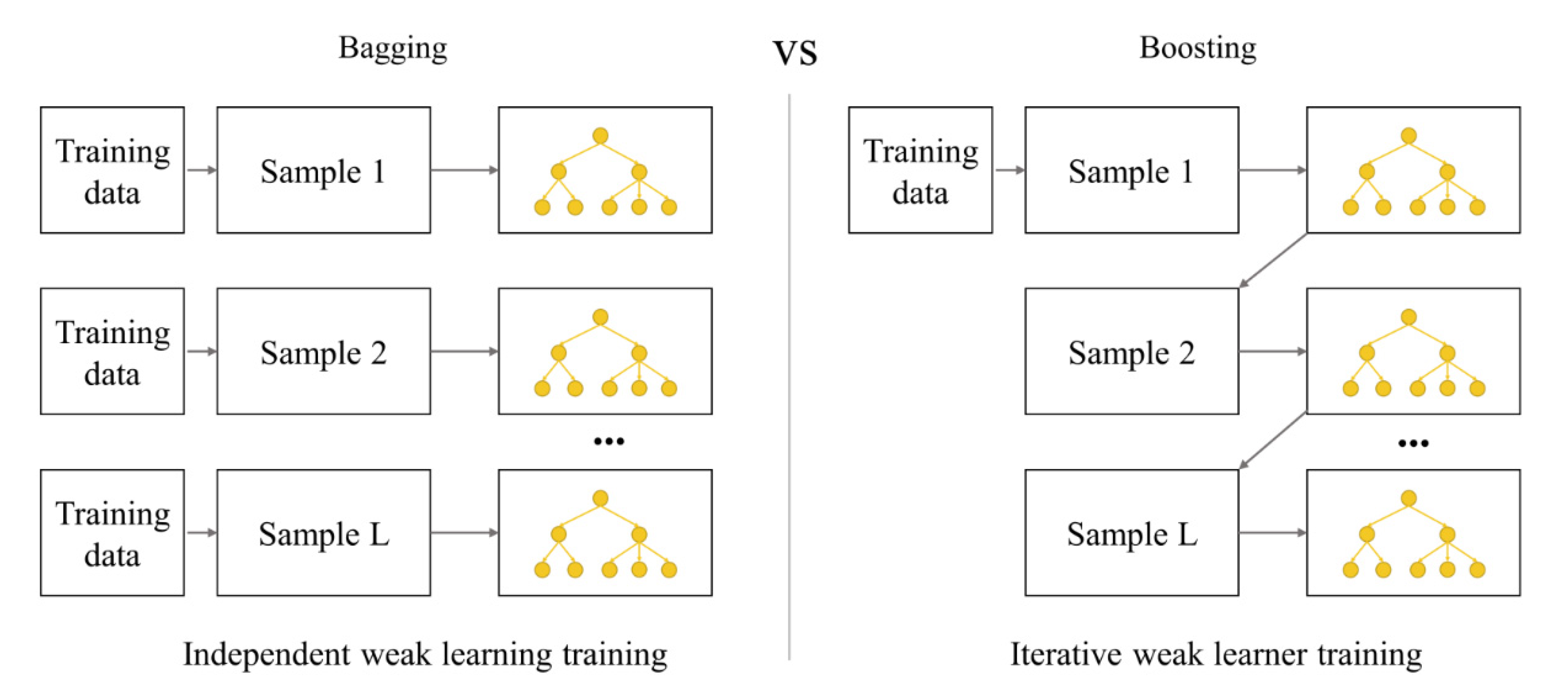
In this section, we explore the principles and properties of random forest (RF) and gradient boosting machine (GBM) algorithms along with the properties of ensembles. Moreover, we explore LOOCV techniques applied for the performance evaluation of models based on small datasets mainly comprising categorical variables used in this study.

2.1. Ensemble Model

Ensemble learning (EL) methods involve combining and building various learning algorithms. This allows ensemble learning algorithms (ELA) to obtain better predictive performance and improved generalization compared to a single learning algorithm [27,28]. Ensemble methods are especially useful when the amount of training data is small. This is because ensemble algorithms (EAs) can reduce the risk of selecting a poor classifier through votes by individual classifiers [29]. Various ensemble techniques have been developed so far, among which bagging and boosting are representative of decision tree (DT)-based ELAs [30,31]. As presented in Figure 1, bagging (also known as bootstrap aggregation [32]) generates numerous bootstraps from the given training data, and an independent predictive model is generated for each bootstrap. Thus, bagging can improve the stability and accuracy of machine learning algorithms (MLA) [33]. Recently, RF has been widely utilized as a bagging method for MLA; Cha et al. and Nguyen et al. [23,34] demonstrated high predictive performance in applying RF to predict waste generation. Boosting, on the other hand, is a technique in which numerous classifiers are generated from early samples, and weak classifiers are collected to generate strong classifiers. As seen in Figure 1, bagging is an independence-based learner training system, while boosting is an iterative and dependence-based system. Boosting is a continuous process of generating classifiers reinforced by weights from weak classifiers from previous stages, which helps reduce the bias and variance of datasets [32]. GBM is representative of boosting DT-based algorithms. Johnson et al. [35] and Kontokosta et al. [36] applied GBM to predict the amount of MSW generation.

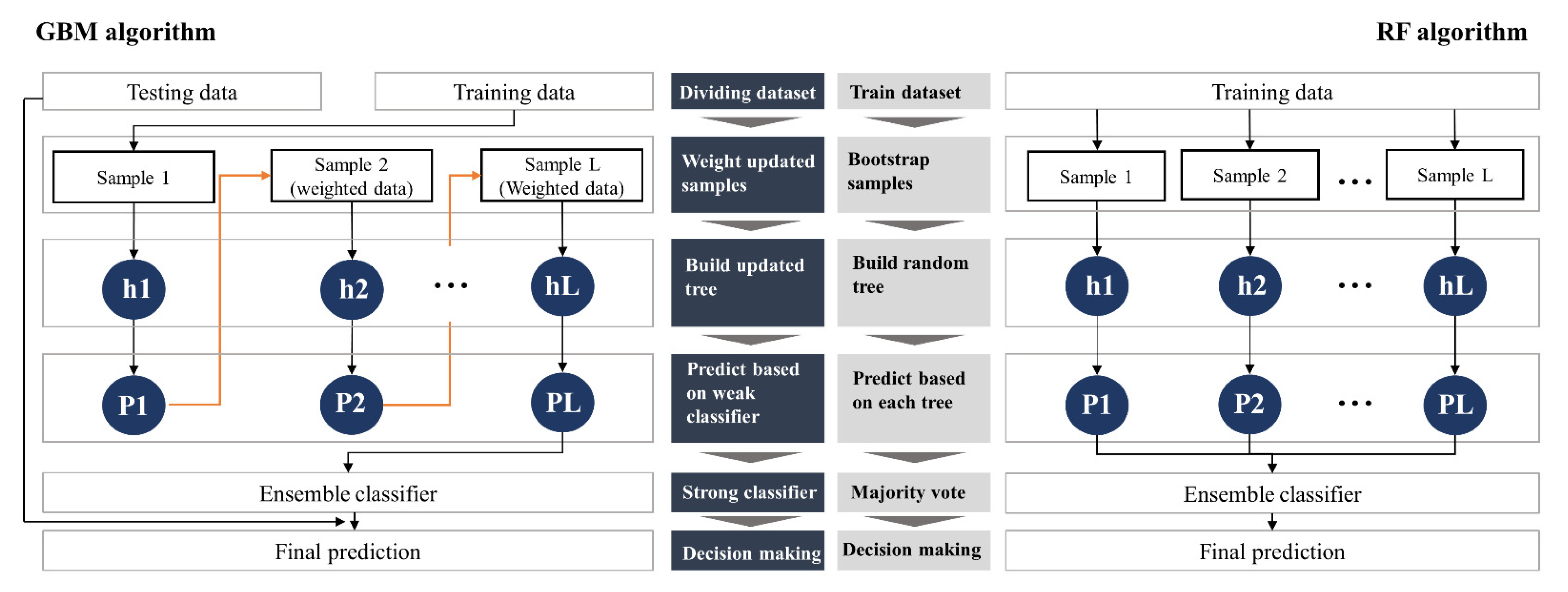
2.2. Gradient Boosting Machine and Random Forest

GBM, as one of the most robust machine learning (ML) algorithms, is widely applied in engineering fields [37] and is a boosting technique. GBM may be deemed a numerical optimization algorithm aimed at finding an additive model that minimizes the loss function. To this end, GBM iteratively adds a new DT (weak classifier in Figure 2), which can reduce the loss function as much as possible at each stage. In other words, at each step, a new DT is fitted to the current residual and added to the previous model to update the residual. As presented in Figure 2, GBM is an iterative and dependence-based algorithm; as it iteratively performs these processes, it increasingly reinforces the classifier by the number of iterations specified by the user. GBM algorithms based on this boosting principle are effective in reducing bias and variance in predictive models [38]. Such characteristics of GBM are deemed useful in solving issues of bias and variance in predictive model results that occur when ML algorithms are applied to small datasets. Therefore, this study utilized GBM to predict demolition waste (DW) generation in a small-dataset environment consisting mainly of categorical variables.
RF is considered among the 10 best classifiers [39]. RF, a representative DT-based algorithm, is a bagging-based ensemble technique that generates bootstrap sampling (Figure 2). RF builds numerous subsets (bootstrap sampling) from the training data and trains the same algorithm several times. The resulting prediction is determined as the mean of all predictions of the submodels. As the number of trees increases, RF can avoid overfitting and be less affected by outliers. Moreover, even when the class is imbalanced, it has superior predictive power over other ML algorithms [33]. Considering these strengths, the application of RF in the data environment utilized in this study (small datasets composed mainly of categorical variables) is also expected to be useful for predicting DW generation.

2.3. Leave-One-Out Cross-Validation (LOOCV)

K-fold and leave-one-out cross-validation (LOOCV) are widely used to evaluate the performance of classification algorithms. For large amounts of data, k-fold cross-validation (CV) should be applied to assess the accuracy of the classification model [40]. LOOCV is a special case of k-fold CV, in which the number of folds is equal to the number of instances (as shown in Figure 3). That is, LOOCV uses all samples in the dataset as the test and training data. The benefit of using so many fitted and evaluated models is a more robust estimate of model performance, as each row of data is given an opportunity to represent the entirety of the test dataset [23]. Therefore, when the number of instances in either a dataset or a class value is small, LOOCV must be applied to verify the accuracy of the classification algorithm [41]. These characteristics of LOOCV were considered in this study when selecting it as the CV method for the performance evaluation of the predictive models.

3. Materials and Methods

3.1. Data Source of Demolition Waste Generation (DWG) Data

This study utilized existing raw data [23,26,42] to develop predictive models for demolition waste (DW) generation. Raw data pertaining to the urban regeneration project districts in Daegu (35.88° N latitude, 128.61° E longitude) and Busan (35.87° N latitude, 128.63° E longitude) in the southern part of Korea were obtained. Therefore, the target buildings surveyed mainly included low-rise detached houses. Table 1 lists the statuses of the buildings whose raw data were used in this study.
Raw data were collected through investigations of the main members, areas, number of floors, structures, material types (i.e., mortar, concrete, block, brick, timber, slate, roofing tile, ceramic and glass, metal, or soil), characteristics, and sizes of the buildings prior to dismantling. These investigations were conducted using teams of two individuals, where one focused on measurements and the other focused on recording the data. The raw data included information on the amount of generation (kg/m2) of 10 types of DW (mortar, concrete, block, brick, timber, slate, roofing tile, ceramic and glass, metal, and soil) from 784 buildings. For each building, information is included on six types of construction characteristics (gross floor area, region, building structure, building use, wall material, and roofing material), which correspond to input variables that affect DW generation. The unit of DW generation data used in this study is kg/m2, in accordance with the following equation:
D W G R i   o f   b u i l d i n g k = A i j   o f   b u i l d i n g G F A   o f   b u i l d i n g k
where DWGR is the demolition waste generation rate (kg/m2), A i j is the amount of waste material j with properties i (kg), and GFA is the gross floor area (m2) of building k.

3.2. Data Preprocessing and Preparing Datasets for Prediction Models

Preprocessing data are necessary to reduce the impact of data distortion or outliers and include cutting, adding, and transforming training datasets [43,44]. A stable dataset construction is required to improve the performance of the predictive model. Therefore, this study performed data outlier elimination and standardization of data to reduce the impact of data distortion and outliers resulting from the large variation in the collected raw data. In this study, the interquartile range method was used to eliminate outliers in the screening of data for use in the models, in accordance with Equation (2). After outlier removal, 690 out of the 784 building samples were used to develop the RF and GBM predictive models in this study.
Q1 − 1.5 × IQR < selecting data < Q3 + 1.5 × IQR,
where IQR is the interquartile range and the value of IQR is Q3 minus Q1, Q1 being the 25th percentile, and Q3 the 75th percentile (Q represents quartile).
Standardization was performed to reduce the impact of data outliers on model performance and to build datasets of the same scales and units. Data standardization was conducted using Equation (3), in which the average of the data was x a v e r a g e and the standard deviation was σ s t a n d a r d   d e v i a t i o n .
x s t a n d a r d i z a t i o n = x e l e m e n t x a v e r a g e σ s t a n d a r d   d e v i a t i o n

3.3. Characteristics and Composition of Variables

Table 2 presents explanations of the data used in this study. Six independent variables and one dependent variable (DW generation) were used to develop the RF and GBM predictive models. The independent variables consist of nominal variables (region, use, structure, wall material, and roofing material) and one numeric variable (GFA). As shown in Table 2, the values converted into scales were utilized as input variables for the nominal variables.

3.4. Application of Machine Learning Techniques

The RF and GBM algorithms were selected to develop predictive models for DW generation for datasets with small samples and were composed mainly of categorical variables. In this study, RF and GBM algorithms were applied to develop 10 models for 10 types of DW, and one model for total DW generation including all 10 types of DW. The RandomForestClassifier [45] and GradientBoostingClassifier [46] packages were used to develop predictive models for DW generation. For optimal performance and evaluation upon application of the algorithm, parameters were tuned for the RF and GBM algorithms, including n_estimators (the number of trees to be grown). The parameters were tuned to maximize each model’s prediction accuracy on the dataset. The optimal settings were determined using the LOOCV process. Explanations of the hyperparameters applied to develop the RF and GBM models in this study are presented in Table 3.

3.5. Model Validation

The LOOCV validation technique was used to validate the models. Because LOOCV puts all samples through tests, it has the advantage of achieving stable results when targeting small datasets compared to the validation set approach, which is an existing cross-validation method (10-fold or k-fold) [23,47]. Several techniques that can be used for model performance evaluation are available. In this study, four statistical metrics (MAE, RMSE, R2, and R) were utilized to verify the performance of the models. Definitions of the performance evaluation metrics are presented in Equations (4)–(7).
MAE = i = 1 n | y i x i | n
RMSE = i = 1 n ( y i x i ) 2 n
R 2 = 1 i = 1 n ( y i x i ) 2 i = 1 n ( y i x ¯ i ) 2
R = i = 1 n ( x i x ¯ i ) ( y i y ¯ i ) i = 1 n ( x i x ¯ i ) 2 i = 1 n ( y i y ¯ i ) 2
where x i is the observed value of the generated DW amount, y i is the predicted value of the generated DW amount, x ¯ i is the mean observed value of the generated DW amounts, y ¯ i is the mean predicted value of the generated DW amount, and n is the number of samples.

4. Results and Discussions

4.1. Model Performance

Figure 4 presents the comparison results of the performance metrics in the 11 predictive models for DW. According to the results of MAE and RMSE values in Figure 4, which indicate the stability of predictive performance, the MAE values of the RF models in all 11 predictive models are lower than those of the GBM models. MAE values are slightly lower in the 10 predictive models for each DW, and also in the total DW production predictive model: the MAE value of the RF model (MAE: 193.7) is lower than that of the GBM model (MAE: 206.2). According to the RMSE results, the GBM models (RMSE value of slate is 0.20, and RMSE value of roofing tile is 34.02) for the slate and roofing tile DW predictive models indicate slightly more stable predictive performance than achieved by the RF model (RMSE value of slate is 2.04, and RMSE value of roofing tile is 34.31). However, the RMSE values of the remaining DW predictive models are lower in the RF model than in the GBM model. The MAE and RMSE results demonstrate that, in the predictive models for small datasets of categorical variables, RF algorithms generally have slightly more reliable predictive performance than achieved by GBM algorithms. In other words, the bagging technique appears to have a slightly better predictive performance in terms of stability over the boosting technique.
Figure 4 shows for each type of DW that RF predictive models (R2 values: 0.34–0.89; R values: 0.73–0.95) are generally superior in terms of the accuracy of predictive performance compared with GBM predictive models (R2 values: 0.22–0.84; R values: 0.71–0.92). Furthermore, from Figure 5, it can be seen that the scatterplots of predicted and observed values of the total DW predictive model conform more closely to ideal prediction lines in the RF model than in the GBM model. However, GBM models demonstrate slightly better predictive performance in terms of accuracy: the R2 and R values for slate are 0.48 and 0.78, respectively, in the GBM model, and 0.46 and 0.77 in the RF model; R2 and R values for roofing tiles are 0.37 and 0.75, respectively, in the GBM model, and 0.37 and 0.74 in the RF model. Considering the models overall, the RF models are slightly superior in terms of the accuracy of DW predictive models, and it is judged that the bagging technique will be more useful than the boosting technique for developing accurate models for small datasets composed of categorical variables.
Meanwhile, the predictive performance based on the type of DW showed different results. This difference can be attributed to the characteristics of the features applied to the model development. In other words, it is expected that more stable performance results can be obtained if the variables affecting waste generation with respect to waste type are included, apart from the six variables used in this study. For instance, the features used in this study (i.e., region, use, structure, GFA, WM, and RM) are considered to be appropriate key features as input variables affecting the amount of soil generation. On the other hand, the ceramic and glass predictive model with the lowest prediction performance requires additional input variables (such as the external window area ratio), apart from the six variables used in this study. Similar findings were also reported for MSW by Johnson et al. [34], who applied the GBM algorithm to apply feature compositions differently and developed predictive models for refuse, paper, and MGP (metal, glass, and plastic). Each predictive model developed in that study showed different R2 and RMSE results depending on the external or internal characteristics of the applied features.

4.2. Comparison of Predictive Models

Although all RF and GBM models developed in this study were derived from a small dataset, the correlation between the actual and predicted values (R value) is 0.7 or higher, demonstrating excellent predictive performance (Figure 4). However, while some DWs (mortar, roofing tile, ceramic, and glass) have slightly lower R2 values (0.4 or lower), their R values are all 0.7 or higher, and thus no issues are expected for the accuracy of the predictive performance. However, these results suggest that it is necessary to include key features considering the characteristics of buildings that affect the DWG for DW types with low predictive performance. In addition, it is expected that this will help improve the R2 value, because this value gradually increases as new variables are introduced into the model [48,49].
Figure 6, Figure 7 and Figure 8 present the comparison results of the observed and predicted DW models using the RF and GMB algorithms; the results for all 11 RF and GBM models indicate that the actual DW generation patterns are well simulated. The mean observed value of the soil predictive model, which had the best predictive performance, is 21.8 kg/m2, while the mean predicted value of the RF model (R value: 0.947) is 21.6 kg/m2, and that of the GBM model (R value: 0.824) is 21.4 kg/m2. The mean observed value of the ceramic and glass predictive model, which had the lowest predictive performance among DW predictive models, is 5.3 kg/ m2, where the mean predicted value of the RF model (R value: 0.729) is 5.4 kg/m2, and that of the GBM model (R value: 0.711) is 5.5 kg/m2. The mean observed value of the total waste predictive model is 1171.2 kg/m2, while the mean predicted value of the RF model (R value: 0.786) is 1169.9 kg/m2, and that of the GBM model (R value: 0.762) is 1166.4 kg/m2. Other predictive models showed results in which the predicted values of the RF and GBM models were close to the observed values. However, as seen in the MAE and RMSE results in Figure 4, the GBM models produced some predicted values that were high compared with values produced by the RF models, indicating that stable predictive performance is somewhat poor (Figure 6, Figure 7 and Figure 8).

4.3. Discussion, Limitations, and Future Work

AI models in previous studies [19,35,50] presented results for some DW types. Johnson et al. [35] applied GBM algorithms to conduct research on refuse, paper, and MGP (metal, glass, and plastic) predictive models. In this study, R2 results for refuse, paper, and MGP spatial models, to which features of external groups were applied, demonstrated predictive performances of 0.604, 0.628, and 0.428, respectively. The predictive performance of MSW and paper predictive models, to which decision tree (DT) algorithms were applied in the study by Kannangara et al. [50], was 0.54 and 0.31, respectively. In the study by Kumar et al. [19], the R2 of the plastic generation predictive model, to which the RF algorithm was applied, demonstrated a predictive performance of 0.66. This study proposes predictive models for the generation of 10 types of DW, and one for total waste generation, for small datasets. In this study, the 11 RF and GBM models developed, despite targeting small datasets, demonstrated excellent predictive performance with the correlation (R) of the observed and predicted values at 0.73–0.95 (RF models) and 0.71–0.92 (GBM models), respectively. R2 values also demonstrated excellent predictive performances of 0.6 or higher, except for mortar, slate, roofing tile, ceramics, and glass. However, as AI models depend on datasets of large sizes [15], a dataset size that is not sufficiently large is a fundamental limitation of this study; obtaining datasets that are sufficiently large is a significant challenge. This study also found significant differences in the performance (MAE, RMSE, R2, R) of predictive models depending on the type of DW, and the R2 values for demolition waste materials such as slate, mortar, roofing tile, ceramic, and glass were relatively low (≤0.5), demonstrating relatively low performance. Johnson et al. [35] suggested that the development of optimal feature groups is also important for improving the predictive performance of AI models by demonstrating that differences in the composition and characteristics of features applied to AI models affect the results of predictive performance. Based on this, it is deemed that further features must be developed to improve the performance of predictive models for the types of DW that had relatively low predictive performance in the present study.

5. Conclusions

This study investigated the development of AI models for DW generation suitable for small datasets composed mainly of categorical variables. The DT-based ensemble model was applied as an algorithm suitable for the datasets, with one selected algorithm being the RF algorithm, which is representative of the bagging technique, and the other being the GBM algorithm representative of the boosting technique. Data preprocessing was performed to improve the stability and accuracy of the models, and the parameters were tuned to fit the RF and GBM algorithms. The LOOCV technique was applied to verify the developed RF and GBM models, and performance evaluation was conducted using statistical metrics such as MAE, RMSE, R2, and R. Therefore, the consideration of AI models developed in this study for small datasets composed mainly of categorical variables, along with the RF and GBM predictive models developed for the generation of 10 types of DW and one for total DW generation, is summarized as follows.
First, for small datasets composed mainly of categorical variables, the bagging technique (RF model) was found to be superior to the boosting technique (GBM model) in terms of the stability and accuracy of predictive performance. However, the GBM model demonstrated excellent predictive performance for certain types of DW (slate and roofing tile). Therefore, the selection of appropriate RF and GBM algorithms, depending on the type of DW, is necessary in developing DW prediction models for small datasets composed mainly of categorical variables.
Second, 11 RF (R2 values: 0.22–0.84; R values: 0.71–0.92) and GBM (R2 values: 0.34–0.89; R values: 0.73–0.95) predictive models under identical conditions demonstrated differences in performance according to the type of DW. This is considered to be due to the characteristics of the features applied in developing the models. Therefore, it is expected that the performance of predictive models will be improved in the future if features matching the characteristics of DW with low predictive performance (mortar, slate, roofing tile, ceramic, and glass, having R2 values ≤0.5) are added.
Finally, it is recommended that RF methods be applied to develop DW predictive models for concrete, block, brick, timber, ceramic and glass, metals, soil, and total waste, while applying GBM models for slate and roofing tiles, based on 11 predictive models developed in this study. This study proposes predictive models for more types of DW than included in the AI models of previous studies. The results of this study are anticipated to be useful tools for building demolition businesses to establish thorough and detailed DW management strategies. For example, based on the predicted amount of waste to be generated from the type of DW, a demolition company can place orders for the required demolition equipment and transportation, which will be of use in minimizing excess costs and personnel allocations.

Author Contributions

Conceptualization, methodology, formal analysis, validation, and supervision, G.-W.C. and H.-J.M.; resources, writing: original draft preparation, writing: review, editing, and funding acquisition, G.-W.C. and Y.-C.K. All authors have read and agreed to the published version of the manuscript.

Funding

This work was supported in part by the National Research Foundation of Korea (NRF) grant funded by the Korean government (MSIT) (NRF-2019R1A2C1088446) and in part by the National Research Foundation of Korea (NRF) grant funded by the Korean government (MSIP) (NRF-2020R1C1C1009061). This work was supported by the Korea Institute of Energy Technology Evaluation and Planning (KETEP) and the Ministry of Trade, Industry & Energy (MOTIE) of the Republic of Korea (No. 20212020800120). This work has supported by the National Research Foundation of Korea (NRF) grant funded by the Korea government (MSIT) (No. NRF-2021R1A2B5B02002699).

Institutional Review Board Statement

Not applicable.

Informed Consent Statement

Not applicable.

Data Availability Statement

The data that support the findings of this study are available from the corresponding author, upon reasonable request.

Conflicts of Interest

The authors declare no conflict of interest.

References

  1. World Health Organization Centre for Health Development; World Health Organization. Hidden Cities: Unmasking and Overcoming Health Inequities in Urban Settings. 2010. Available online: https://www.who.int/publications/i/item/9789241548038 (accessed on 12 May 2021).
  2. Leão, S.; Bishop, I.; Evans, D. Spatial–Temporal Model for Demand and Allocation of Waste Landfills in Growing Urban Regions. Comput. Environ. Urban Syst. 2004, 28, 353–385. [Google Scholar] [CrossRef]
  3. World Bank. What a Waste 2.0: A Global Snapshot of Solid Waste Management to 2050; International Bank for Reconstruction and Development/World Bank: Washington, DC, USA, 2018. [Google Scholar]
  4. Llatas, C. A Model for Quantifying Construction Waste in Projects According to the European Waste List. Waste Manag. 2011, 31, 1261–1276. [Google Scholar] [CrossRef] [PubMed]
  5. Li, J.; Ding, Z.; Mi, X.; Wang, J. A Model for Estimating Construction Waste Generation Index for Building Project in China. Resour. Conserv. Recycl. 2013, 74, 20–26. [Google Scholar] [CrossRef]
  6. Wang, J.; Li, Z.; Tam, V.W.Y. Identifying Best Design Strategies for Construction Waste Minimization. J. Clean. Prod. 2015, 92, 237–247. [Google Scholar] [CrossRef]
  7. Lu, W.; Yuan, H.; Li, J.; Hao, J.J.; Mi, X.; Ding, Z. An Empirical Investigation of Construction and Demolition Waste Generation Rates in Shenzhen City, South China. Waste Manag. 2011, 31, 680–687. [Google Scholar] [CrossRef] [PubMed] [Green Version]
  8. Butera, S.; Christensen, T.H.; Astrup, T.F. Composition and Leaching of Construction and Demolition Waste: Inorganic Elements and Organic Compounds. J. Hazard. Mater. 2014, 276, 302–311. [Google Scholar] [CrossRef]
  9. Banias, G.; Achillas, C.; Vlachokostas, C.; Moussiopoulos, N.; Papaioannou, I. A Web-Based Decision Support System for the Optimal Management of Construction and Demolition Waste. Waste Manag. 2011, 31, 2497–2502. [Google Scholar] [CrossRef]
  10. Song, Y.; Wang, Y.; Liu, F.; Zhang, Y. Development of a Hybrid Model to Predict Construction and Demolition Waste: China as a Case Study. Waste Manag. 2017, 59, 350–361. [Google Scholar] [CrossRef]
  11. Lu, W.S.; Yuan, H.P. A Framework for Understanding Waste Management Studies in Construction. Waste Manag. 2011, 31, 1252–1260. [Google Scholar] [CrossRef] [Green Version]
  12. Hurley, J.W. Valuing the Pre-Demolition Audit Process. In Proceedings of the 11th Rinker International Conference (CIB report 287), Gainesville, FL, USA, 7–10 May 2003; pp. 151–164. Available online: https://www.cce.ufl.edu/wp-content/uploads/2012/08/Deconstruction_and_Materials_Reuse.pdf (accessed on 3 May 2021).
  13. Nagalli, A. Estimation of construction waste generation using machine learning. Proc. Inst. Civ. Eng. Waste Resour. Manag. 2021, 174, 22–31. [Google Scholar]
  14. Coskuner, G.; Jassim, M.S.; Zontul, M.; Karateke, S. Application of Artificial Intelligence Neural Network Modeling to Predict the Generation of Domestic, Commercial and Construction Wastes. Waste Manag. Res. 2021, 39, 499–507. [Google Scholar] [CrossRef]
  15. Abdallah, M.; Abu Talib, M.A.; Feroz, S.; Nasir, Q.; Abdalla, H.; Mahfood, B. Artificial Intelligence Applications in Solid Waste Management: A Systematic Research Review. Waste Manag. 2020, 109, 231–246. [Google Scholar] [CrossRef] [PubMed]
  16. Golbaz, S.; Nabizadeh, R.; Sajadi, H.S. Comparative Study of Predicting Hospital Solid Waste Generation Using Multiple Linear Regression and Artificial Intelligence. J. Environ. Health Sci. Eng. 2019, 17, 41–51. [Google Scholar] [CrossRef]
  17. Noori, R.; Karbassi, A.; Salman Sabahi, M.S. Evaluation of PCA and Gamma Test Techniques on ANN Operation for Weekly Solid Waste Prediction. J. Environ. Manag. 2010, 91, 767–771. [Google Scholar] [CrossRef] [PubMed]
  18. Abbasi, M.; Abduli, M.A.; Omidvar, B.; Baghvand, A. Forecasting Municipal Solid Waste Generation by Hybrid Support Vector Machine and Partial Least Square Model. Int. J. Environ. Resour. 2013, 7, 27–38. [Google Scholar]
  19. Kumar, A.; Samadder, S.R.; Kumar, N.; Singh, C. Estimation of the Generation Rate of Different Types of Plastic Wastes and Possible Revenue Recovery from Informal Recycling. Waste Manag. 2018, 79, 781–790. [Google Scholar] [CrossRef] [PubMed]
  20. Abdoli, M.A.; Nezhad, M.F.; Sede, R.S.; Behboudian, S. Longterm Forecasting of Solid Waste Generation by the Artificial Neural Networks. Environ. Prog. Sustain. Energy 2011, 31, 628–636. [Google Scholar] [CrossRef]
  21. Azadi, S.; Karimi-Jashni, A. Verifying the Performance of Artificial Neural Network and Multiple Linear Regression in Predicting the Mean Seasonal Municipal Solid Waste Generation Rate: A Case Study of Fars Province, Iran. Waste Manag. 2016, 48, 14–23. [Google Scholar] [CrossRef] [PubMed]
  22. Chhay, L.; Reyad, M.A.H.; Suy, R.; Islam, M.R.; Mian, M.M. Municipal Solid Waste Generation in China: Influencing Factor Analysis and Multi-Model Forecasting. J. Mater. Cycles Waste Manag. 2018, 20, 1761–1770. [Google Scholar] [CrossRef]
  23. Cha, G.W.; Moon, H.J.; Kim, Y.M.; Hong, W.H.; Hwang, J.H.; Park, W.J.; Kim, Y.C. Development of a Prediction Model for Demolition Waste Generation Using a Random Forest Algorithm Based on Small DataSets. Int. J. Environ. Res. Public Health 2020, 17, 6997. [Google Scholar] [CrossRef]
  24. Raschka, S. Model Evaluation, Model Selection, and Algorithm Selection in Machine Learning. Comput. Res. Repos. 2018, 1811, 12808. [Google Scholar]
  25. Jiang, Y.; Lin, J.; Cukic, B.; Menzies, T. Variance Analysis in Software Fault Prediction Models. In Proceedings of the ISSRE’09: 20th I.E.E.E. international Conference on Software Reliability Engineering, Bengaluru, India, 16–19 November 2009; pp. 99–108. [Google Scholar]
  26. Cha, G.W.; Kim, Y.C.; Moon, H.J. New Approach for Forecasting Demolition Waste Generation Using Chi-Squared Automatic Interaction Detection (CHAID) Method. J. Clean. Prod. 2017, 168, 375–385. [Google Scholar] [CrossRef]
  27. Opitz, D.; Maclin, R. Popular Ensemble Methods: An Empirical Study. J. Artif. Intell. Res. 1999, 11, 169–198. [Google Scholar] [CrossRef]
  28. Ghimire, B.; Rogan, J.; Galiano, V.R.; Panday, P.; Neeti, N. An Evaluation of Bagging, Boosting, and Random Forests for Land-Cover Classification in Cape Cod, Massachusetts, USA. GISci. Remote Sens. 2012, 49, 623–643. [Google Scholar] [CrossRef]
  29. Dietterich, T.G. An Experimental Comparison of Three Methods for Constructing Ensembles of Decision Trees: Bagging, Boosting, and Randomization. Mach. Learn. 2000, 40, 139–157. [Google Scholar] [CrossRef]
  30. Zhou, Z.H. Ensemble Methods; Foundations and Algorithms; CRC Press: Boca Raton, FL, USA; London, UK; New York, NY, USA, 2012. [Google Scholar]
  31. Van der Laan, M.J.; Polley, E.C.; Hubbard, A.E. Super Learner. Stat. Appl. Genet. Mol. Biol. 2007, 6, 25. [Google Scholar] [CrossRef]
  32. Breiman, L. Bagging Predictors. Mach. Learn. 1996, 24, 123–140. [Google Scholar] [CrossRef] [Green Version]
  33. Breiman, L. Random Forests. Mach. Learn. 2001, 45, 5–32. [Google Scholar] [CrossRef] [Green Version]
  34. Nguyen, X.C.; Nguyen, T.T.H.; La, D.D.; Kumar, G.; Rene, E.R.; Nguyen, D.D.; Chang, S.W.; Chung, W.J.; Nguyen, X.H.; Nguyen, V.K. Development of Machine Learning—Based Models to Forecast Solid Waste Generation in Residential Areas: A Case Study from Vietnam. Resour. Conserv. Recycl. 2021, 167, 105381. [Google Scholar] [CrossRef]
  35. Johnson, N.E.; Ianiuk, O.; Cazap, D.; Liu, L.; Starobin, D.; Dobler, G.; Ghandehari, M. Patterns of Waste Generation: A Gradient Boosting Model for Short-Term Waste Prediction in New York City. Waste Manag. 2017, 62, 3–11. [Google Scholar] [CrossRef]
  36. Kontokosta, C.E.; Hong, B.; Johnson, N.E.; Starobin, D. Using Machine Learning and Small Area Estimation to Predict Building-Level Municipal Solid Waste Generation in Cities. Comput. Environ. Urban Syst. 2018, 70, 151–162. [Google Scholar] [CrossRef]
  37. Qi, C.; Tang, X. Slope Stability Prediction Using Integrated Metaheuristic and Machine Learning Approaches: A Comparative Study. Comput. Ind. Eng. 2018, 118, 112–122. [Google Scholar] [CrossRef]
  38. Friedman, J.H. Greedy Function Approximation: A Gradient Boosting Machine. Ann. Stat. 2001, 29, 1189–1232. [Google Scholar] [CrossRef]
  39. Fernandez-Delgado, M.; Cernadas, E.; Barro, S.; Amorim, D. Do We Need Hundreds of Classifiers to Solve Real World Classification Problems? J. Mach. Learn. Res. 2014, 15, 3133–3181. [Google Scholar]
  40. Witten, I.H.; Frank, E.; Hall, M.A. Data Mining: Practical Machine Learning Tools and Techniques, 3rd ed.; Morgan Kaufmann: Waltham, MA, USA, 2011. [Google Scholar]
  41. Wong, T.T. Performance Evaluation of Classification Algorithms by k-Fold and Leave-One-Out Cross Validation. Pattern Recognit. 2015, 48, 2839–2846. [Google Scholar] [CrossRef]
  42. Cha, G.W.; Moon, H.J.; Kim, Y.C.; Hong, W.H.; Jeon, G.Y.; Yoon, Y.R.; Hwang, C.; Hwang, J.H. Evaluating Recycling Potential of Demolition Waste Considering Building Structure Types: A Study in South Korea. J. Clean. Prod. 2020b, 256, 120385. [Google Scholar] [CrossRef]
  43. Kuhn, M.; Johnson, K. Applied Predictive Modeling; Springer: New York, NY, USA, 2013; pp. 27–59. [Google Scholar]
  44. Nisbet, R.; Elder, J.; Miner, G. Handbook of Statistical Analysis and Data Mining Applications; Academic Press: Cambridge, MA, USA, 2009. [Google Scholar]
  45. RandomForestClassifier. Available online: https://scikit-learn.org/stable/modules/generated/sklearn.ensemble.RandomForestClassifier.html (accessed on 15 May 2021).
  46. GradientBoostingClassifier. Available online: https://scikit-learn.org/stable/modules/generated/sklearn.ensemble.GradientBoostingClassifier.html (accessed on 15 May 2021).
  47. Shao, Z.; Er, M.J. Efficient Leave-One-Out Cross-Validation-Based Regularized Extreme Learning Machine. Neurocomputing 2016, 194, 260–270. [Google Scholar] [CrossRef]
  48. Carter, D.S. Comparison of different shrinkage formulas in estimating the population multiple correlation coefficients. Educ. Psychol. Meas. 1979, 39, 261–266. [Google Scholar] [CrossRef]
  49. Fan, X. Statistical significance and effect size in education research: Two sides of a coin. J. Educ. Res. 2001, 94, 275–282. [Google Scholar] [CrossRef]
  50. Kannangara, M.; Dua, R.; Ahmadi, L.; Bensebaa, F. Modeling and Prediction of Regional Municipal Solid Waste Generation and Diversion in Canada Using Machine Learning Approaches. Waste Manag. 2018, 74, 3–15. [Google Scholar] [CrossRef]
Figure 1. Workflows of bagging and boosting methods.
Ijerph 18 08530 g001
Figure 2. Comparison of the structure and workflows of the gradient boosting machine (GBM) and random forest (RF) algorithms.
Ijerph 18 08530 g002
Figure 3. Schematic representation of the leave-one-out cross-validation (LOOCV) method.
Ijerph 18 08530 g003
Figure 4. Comparison of statistical metrics (MAE, RMSE, R2, R) for GBM and RF models developed in this study. MAE, mean absolute error; RMSE, root mean square error; R2, coefficient of determination; R, Pearson’s correlation coefficient.
Ijerph 18 08530 g004
Figure 5. Scatter plot of the observed and predicted total DW generation rate including all waste types using GBM and RF.
Ijerph 18 08530 g005
Figure 6. Comparison of the observed and predicted DW generation (kg/m2) with the estimated ML models using RF and GBM for mortar, concrete, block, and brick.
Ijerph 18 08530 g006
Figure 7. Comparison of the observed and predicted DW generation (kg/m2) with the estimated ML models using RF and GBM for timber, slate, roofing tile, and ceramics & glass.
Ijerph 18 08530 g007
Figure 8. Comparison of the observed and predicted DW generation (kg/m2) with the estimated ML models using RF and GBM for metal, soil, and total waste.
Ijerph 18 08530 g008
Table 1. Building status of raw data used in this study.
Structure TypeNumber of BuildingsTotal Floor Area (m2)
RC14756,929
Masonry35233,291
Wood28522,750
Total 784112,970
Table 2. Input and output variables used to develop the models in this study.
Variables
Type
VariablesDescriptionUnit or Scale of Variables
Independent variablesRegionNominal variable;
Areas where DW has occurred;
Three region variables (Region A, B, C)
Region A is 1
Region B is 2
Region C is 3
Building useNominal variable;
Usage of building where DW has occurred;
Three usage variables (residential-only,
commercial and residential, commercial-only)
Residential-only is 1
Commercial and Residential is 2
Commercial-only is 3
Building structureNominal variable;
Structure of building where DW has occurred;
Three structure variables (reinforced concrete, masonry, wooden)
Reinforced concrete is 1
Masonry is 2
Wooden is 3
Wall materialNominal variable;
Main wall material of building where DW has occurred;
Four wall material variables (reinforced concrete wall,
brick wall, block wall, wall made of soil)
Reinforced concrete wall is 1
Brick wall is 2
Block wall is 3
Wall made of soil is 4
Roofing materialNominal variable;
Main roofing material of building where DW has occurred;
Four roofing material variables (slab, slab and roofing tile, roof with asbestos, roofing tile)
Slab is 1
Slab and roofing tile is 2
Roof with asbestos is 3
Roofing tile is 4
Gross floor area (GFA)Numeric variablem2
Dependent
variable
Waste generationNumeric variablekg/m2
Table 3. Hyperparameters tuned in RF and GBM algorithms.
AlgorithmParameterDefinitionApplied Value or Reference
RFcriterionQuality measurement of a splitMean squared error
n_estimatorsThe number of trees in the forest500
min_samples_splitThe minimum number of samples required to split an internal node2
min_samples_leafThe minimum number of samples required to be at a leaf node1
max_depthThe maximum depth of the treeMaximum possible
GBMcriterionQuality measurement of a splitMean squared error
n_estimatorsThe number of boosting stages500
min_samples_splitThe minimum number of samples required to split an internal node2
lossLeast squaresLeast squares
learning rateAmount of learning0.1
subsampleRate of sampling data to control overfitting1.0
Publisher’s Note: MDPI stays neutral with regard to jurisdictional claims in published maps and institutional affiliations.

