Article

Impact of Income, Density, and Population Size on PM2.5 Pollutions: A Scaling Analysis of 254 Large Cities in Six Developed Countries

1
Department of Business, Gachon University, 1342 Seongnam-daero, Sujung-gu, Seongnam 13120, Gyeonggi-do, Korea
2
Gachon Center for Convergence Research, Gachon University, 1342 Seongnam-daero, Sujung-gu, Seongnam 13120, Gyeonggi-do, Korea
*
Author to whom correspondence should be addressed.
Int. J. Environ. Res. Public Health 2021, 18(17), 9019; https://doi.org/10.3390/ijerph18179019
Submission received: 15 July 2021 / Revised: 20 August 2021 / Accepted: 22 August 2021 / Published: 26 August 2021

Abstract

:
Despite numerous studies on multiple socio-economic factors influencing urban PM2.5 pollution in China, only a few comparable studies have focused on developed countries. We analyzed the impact of three major socio-economic factors (i.e., income per capita, population density, and population size of a city) on PM2.5 concentrations for 254 cities from six developed countries. We used the Stochastic Impacts by Regression on Population, Affluence and Technology (STIRPAT) model with three separate data sets covering the period of 2001 to 2013. Each data set of 254 cities were further categorized into five subgroups of cities ranked by variable levels of income, density, and population. The results from the multivariate panel regression revealed a wide variation of coefficients. The most consistent results came from the six income coefficients, all of which met the statistical test of significance. All income coefficients except one carried negative signs, supporting the applicability of the environmental Kuznet curve. In contrast, the five density coefficients produced statistically significant positive signs, supporting the results from previous studies. However, we discovered an interesting U-shaped distribution of density coefficients across the six subgroups of cities, which may be unique to developed countries with urban pollution. The results from the population coefficients were not conclusive, which is similar to the results of previous studies. Implications from the results of this study for urban and national policy makers are discussed.

1. Introduction

Heavy fine particulate (PM2.5) pollution has increased and become a high risk to public health in densely populated urban areas in many countries. According to a recent study involving 381 large cities with populations of more than 0.75 million people in China, India, the U.S., Europe, Latin America, and Africa [1], the annual average PM2.5 concentrations from 2000 to 2006 in 23.9% of these cities was higher than the World Health Organization’s (WHO) interim Target 1 of less than 35 micrograms per cubic meter (35 μg/m3). In addition, only 18.0% of these large cities were within the recommended WHO target of less than 10 μg/m3. Large cities in Asia, especially China and India, had the worst record, with 48.7% of these cities recording PM2.5 concentrations higher than 35 μg/m3 and only 1.7% with PM2.5 concentrations of less than 10 μg/m3. In contrast, large cities in Latin America had the best air quality, with 64.4% of them within the 10 μg/m3 guideline.
Translating urban pollution risk in terms of the number of people, it has been reported [1] that more than 500 million Chinese urban residents (14% of the global urban population) were at risk from PM2.5 hazard (35 μg/m3 or more) in 2010. These people resided in 154 cities, which represented 78% of all large cities with a population of more than 1 million. To make matters worse, 278 million more people became exposed to PM2.5 hazards between 2000 and 2010 due to the high birth rate and high migration rate from rural areas to these cities.
In short, the air pollution risk appears to be far more serious in urban settings in large cities in several countries in Asia, particularly in China, India, and Pakistan. Therefore, a high priority for research on socio-economic influencing factors of PM2.5 pollution in urban centers is needed to develop effective mitigating policies to control urban pollution. However, the unavailability of relevant city-wide technology-related data, such as the industrial structure, energy intensity, service structure, vehicle usage, as well as income per capita has been a barrier to the productive flow of research. Fortunately, however, the unavailability of city-wide data has become somewhat more manageable in recent years, increasing the number of necessary studies.
A large majority of these studies have focused exclusively on urban pollution in China [2,3,4,5,6,7,8,9,10,11,12]. For example, Hao and Liu [2] examined the four influencing factors of GDP per capita, industrial structure, vehicle population, and population density to PM2.5 concentrations for 73 Chinese cities. The results showed that secondary industries, including manufacturing, construction, fast moving consumer goods, and other industries, and the vehicle population, in that order, had greater impacts on PM2.5 concentrations in these cities. Wu et al. [3] used PM2.5 data from the same 73 cities in 2013 and 2014 and determined that PM2.5 significantly correlated with the proportion of industrial activity, the number of vehicles, and household gas consumption in these cities.
Expanding the number of cities to 338 Chinese cities from 2014 to 2017, Wang et al. [5] determined that population density and the number of vehicles had a large impact on increasing PM2.5, and GDP per capita had a moderate impact on PM2.5. Cheng et al. [4] also used STIRPAT models to analyze influencing factors of PM2.5 concentrations for 285 Chinese cities from 2001 to 2012. Their results indicated that population density, income, and traffic intensity had a significant impact on PM2.5 concentrations. In addition, secondary industries and central heating significantly aggravated urban air pollution. However, foreign direct investment was not a significant factor.
In contrast to the many studies on urban pollution, only a few socio-economic studies on PM2.5 concentrations in cities in developed countries have been published in recent years [13,14]. The current study fills this important gap in the urban pollution literature for developed economies by focusing on 254 cities in the U.S., Germany, Japan, France, U.K. and Spain. More specifically, a STIRPAT framework was used to analyze the three influencing factors of population, income, and technology on PM2.5 concentrations from 2001 to 2013.
After this introduction, the paper has four sections. A brief literature review on selected socio-economic studies on PM2.5 pollution is presented in the next section, followed by a section explaining the STIRPAT model and data sources. An analysis of the results is presented in the fourth section. Finally, the conclusion, implications, and limitations of the study are presented in the fifth section.

2. Literature Review of PM2.5 Concentrations in Urban Centers

The large majority of socio-economic studies on PM2.5 concentration in urban centers in recent years have concentrated on China [2,3,4,5,6,8,9,10,12,15]. One reason is that PM2.5 is the main component of haze and fog for large cities in China, so investigating the relationship between socio-economic factors related to PM2.5 pollution is very important to Chinese policy makers. Another reason is that city-level data for PM2.5 pollutants and related socio-economic factors in many other developing countries are mostly unavailable. In terms of developed countries, PM2.5 is not as critical of an environmental pollution issue for cities in developed countries [2]. Thus, only a few socio-economic studies on PM2.5 concentrations for cities in developed countries have been published recently on cities in the U.S. [13] and Germany [14]. A group of related studies on air pollution in developed countries such as the U.S. and Canada have also been published [16,17,18,19,20,21]. A few other papers on multiple cities in both developed and developing countries have also been published [1,22,23].
We selected the five most representative papers on the socio-economic analysis of city-level PM2.5 concentrations in China for a closer examination [2,4,8,9,15]. The results show that economic development measured by city GDP per capita and population density are the two most influential factors analyzed by these five studies, followed by traffic intensity analyzed by four articles, and industrial structure and energy or electricity intensity examined by three articles. Other factors such central heating, trade openness, and foreign direct investment were analyzed in one article each.
The most consistent finding is related to the increasing or decreasing impact of city GDP per capita to PM2.5 concentrations, depending on the income level of cities. All five articles found a statistically significant inverse U-shaped or inverted N-shaped environmental Kuznet curve (EKC). For example, Cheng et al. [4] estimated that 83.4% of Chinese cities are below the inflection point of EKC, and as a result of increasing income, have experienced an increase in PM2.5 pollution. Similarly, Liu et al. [9] concluded that high- income cities in China have surpassed the peak of their EKC while upper- and low-middle income cites have not.
Wu et al. [8] also estimated that most cities in the eastern region with higher incomes have passed the inflection point, while cities in the middle region may need 10 to 15 years to reach their peak of EKC. To elaborate, Wu et al. [8] verified the existence of an inverted U-shaped EKC involving 104 cities in the middle region of China with the inflection point estimated at $18,506 per capita. As of 2011, only 11% (13) of these cities have arrived at this inflection point, creating a win-win relationship between income and PM2.5 pollution. For 108 cities in the eastern region, there is an inverted N-shaped curve with a projected inflection point of $9186. As many as 64% (69) of the cities have reached their inflection point, and another 18% (19) cities are expected to reach their inflection point within the next five years. The remaining 47 cities in the western region do not follow the EKC and show a linear positive relationship between income per capita and PM2.5 pollution.
Wang and Fang’s [6] study on 53 cities in the Bohai Rim Urban Agglomeration found that 43 of the 53 cities displayed a negative relationship with GDP per capita with an average coefficient of −1.8. In other words, an increase of 10,000-yuan GDP per capita would cause a reduction of 1.18% of μg/m3 in PM2.5.
Nearly the same findings can be found for industrial structure, measured by the proportion of value added by secondary industry to GDP as well as traffic intensity measured by the proportion of the number of civilian vehicles to the total length of urban roads. In short, four of the five articles (with the exception of Wu et al. [8]) confirmed a positive and significant relationship between high traffic intensity and high secondary industry output to higher PM2.5 concentrations.
The impact of population density on PM2.5 pollution has had somewhat contradictory results in these five articles. The findings by Cheng et al. [4], Wu et al. [8], and Zhou et al. [15] were statistically significant and positive. For example, Cheng et al. [4] showed that population density coefficients to PM2.5 concentrations derived from three separate panel regression models for 285 cities in China from 2001 to 2012 generated all six population density coefficients ranging from +0.06 to +0.029, which were statistically significant at the 1% level. In other words, a 1% increase in density increased PM2.5 concentrations from 0.029% to 0.06%, while the effects from other factors such as income, industrial structure, electricity intensity, traffic intensity, and several others held constant. The other two articles by Hao and Liu [2] and Lin et al. [24] showed positive but no statistically significant density coefficients.
Another factor, energy or electricity intensity, has also generated somewhat contradictory findings in the three articles. For example, Cheng et al. [4] found a statistically significant positive impact of increased electricity consumption on increased PM2.5 pollution. Similarly, Wu et al. [8] found a strong positive impact of coal consumption on PM2.5 pollution. In contrast, Zhou et al. [15] found no significant relationship between electricity consumption and PM2.5 pollution.
It is interesting to note that none of the five articles examined the impact of the population size of cities on PM2.5 pollution. However, other papers such as Wang et al. [25] reported a positive correlation between PM2.5 concentrations and urban population, together with the size of the urban areas, the share of secondary industry, and population density. Han et al. [11] and Han et al. [26] suggested that urbanization had a considerable impact on increasing PM2.5 concentrations in Chinese cities.
The findings from socio-economic analyses of urban PM2.5 pollution in developed countries are less clear as they vary from those reported on city level PM2.5 concentrations in China. A recent socio-economic analysis of PM2.5 pollution on cites in developed countries emphasized the role of population density over income or population size. For example, Carozzi and Roth [13] found a positive and statistically significant population density coefficient of +0.13 for PM2.5 concentrations. Specifically, they found that doubling the density would increase the average PM2.5 pollution roughly 10% across 933 U.S. cities.
In another systematic study on 109 districts in Germany, which included 51 urban districts, Borck and Schrauth [14] found that a 1% increase in population density increased PM2.5 concentrations by a modest 0.08%. Using an authoritative survey, Ahlfeldt and Pietrostefani [27] cited both studies by Carozzi and Roth [13] and Borck and Schrauth [14], and recommended +0.13 as the elasticity for pollution reduction. In short, the impact of high-density cities on PM2.5 pollution was positive in Chinese studies. Similarly, studies on U.S. and Germany cities also suggested that the effect of high population density was moderately positive.
However, when population density is examined in the framework of urban spatial structure or urban form in relation to air pollution, studies of American and European cities have shown that low-density urban sprawl can lead to a significant deterioration of air quality [16,19,28,29].
For example, Bereitsnaft and Debbaze [19] found that among 86 metropolitan areas in the U.S., low-density urban sprawls led to higher concentration of air pollution. Stone [16] showed for the 45 major cities in the U.S, the more compact the city, the smaller the spread, the more likely it was to reduce air pollution emissions. The primary reason is that compact low-density cities can reduce transportation emissions and air pollution, due to the proximity of housing and employment. In contrast, Clark et al. [30] found that PM2.5 pollution levels increase as population density increases. Another study for 249 European cities found that high density cities were more vulnerable to high levels of SO2 concentration [31].
In sum, it is likely that both very high- and very low-density cities may be subjected to higher levels of air pollution emissions. Thus, several recent studies have proposed adjusting population density upward by promoting monocentric urban structures for those low-density cities while adjusting population density downwards by promoting polycentric structures for the excessively high-density cities as possible remedies to reduce air pollution [32,33,34].
As for the impact of income on PM2.5 pollution, Anenberg et al. [22] discovered that PM2.5 concentrations across 82 global cities were negatively associated with city GDP per capita at a correlation coefficient of 0.64 at p < 0.0001. In other words, the negative impact from higher income cities in developed countries on PM2.5 pollution appears to be more pervasive compared to Chinese cities.
Another paper by Ouyang et al. [35] examined the driving forces of PM2.5 concentrations in 30 OECD countries from 1998 to 2015 using a threshold panel model. The result was that a 1% increase in GDP per capita decreased the PM2.5 concentrations from 0.3% to 0.4%, depending on the three income levels of countries. These findings supported the earlier studies by Wang and Fang [6] and Wang et al. [25].
As for the impact of population size of a city on PM2.5 pollution, Han et al. [1] discovered an inverse U-shape relation among Chinese cities. However, they indicated that the relationships in U.S., European, and Latin American cities were stationary or showed a small increasing trend. In other words, the larger population size cities in China may be more likely to experience higher PM2.5 pollution than those in U.S., European, and Latin American cities. For cities in India and Africa, they discovered a U-shaped trend for PM2.5 concentrations as urban population increased.

3. Method and Data

3.1. STIRPAT Model

Many scholars have used econometric models to analyze the influencing factors of energy usage and air pollution from a socio-economic perspective. Econometric models include both cross-section and panel models. The use of panel models has become popular as they can increase the sample size, reduce collinearity between variables, and control individual heterogeneity of samples to improve the reliability and validity of the estimates [4].
The original IPAT model was refined later to become the Stochastic Impacts by Regression on Population, Affluence and Technology (STIRPAT) model, which enabled researchers to estimate the proportional change of the environmental impact per given proportional change in population, affluence, and technology.
The STIRPAT model is defined as
I i t = a P i t b A i t c T i t d e i t
where I represents the pollution intensity of a pollutant, P represents the total population, A depicts affluence or income, and T indicates the level of technological development. Subscript i and t of each variable denote the cross-sectional unit, which is the cites and time period, respectively; a is the constant; b, c, and d are the exponents of P, A, and T, respectively, to be estimated; and e is the residual error term.
To ease the task of estimating exponents, Equation (1) is converted into the log-log form of Equation (2) by taking the natural log of both sides.
I n I i t = I n a i t + b I n P i t + c I n A i t + d I n ( T i t ] + e i t
The natural log is helpful as it converts non-linear variables to linear ones, rendering the results interpretable as a percentage change. For example, b can be viewed as the population elasticity that measures the percentage change of the environmental impact resulting from a 1% change in population. The STIRPAT model has also been used to examine the impact of population, income, and/or technology in other areas such as the material footprint, human ecological footprint, and environmental efficiency of well-being [36,37,38].
Many scholars have also used the STIRPAT model to analyze the impact of socio-economic factors on PM2.5 pollution at the country level as well as the city level [39,40,41,42,43,44,45,46]. As for a measure for technology, there is no consensus on a single measure of technology [47]. According to Cole and Neumayer [48], technology is a broad term intended to reflect technological, cultural, and institutional determinants of the environmental impact. For example, Uddin, Alam and Gow [49] extensively used the urbanization ratio measured as the percentage of the population living in urban areas for technology in their STIRPAT model. Wang et al. [40] also used the urbanization ratio, together with energy intensity for the technology factor in their STIRPAT model.
For this study, population density is used to represent the technology factor in the STIRPAT model, together with the population size of a city as P and income per capita of a city as A, as shown in Equation (3):
I n Y i t = I n a + b I n P i t + c I n A i t + d I n P D i t + e i t
where P represents the population size of each city, A represents the GDP per capita of a city, and PD represents population density calculated by population per km2.
In addition, we use threshold regression as a robust test to verify the results from the STIRPAT analysis. This study uses Hansen’s [50] threshold regression using the simplest form of regression where a single threshold was called for. The single threshold regression model includes Equations (4) and (5):
Y i = θ 1 x i + e i   q i γ
Y i = θ 2 x i + e i   q i > γ
where i represents the units of analysis, which is a city; Y represents the dependent variable of PM2.5 concentrations; x represents the explaining variables of population size (P), income per capita (I), and population density (PD); θ1 and θ2 represent parameters to be estimated; q represents the threshold variable; γ represents the threshold quantity; and e represents the error term. Based on the variables selected in this study, the threshold model is expressed in Equations (6) and (7):
I n Y i = θ 1 I n P i + I n I i + I n P D i + e i   ,   I n q i I n γ
I n Y i = θ 2 I n P i + I n I i + I n P D i + e i   ,   ( I n q i > I n γ )
We then combine Equations (6) and (7) using a dummy variable, which takes the value of one when the condition in parentheses is met, otherwise it becomes zero. This combined equation is used as the estimation equation of this research. The generalized threshold panel model has been used extensively in the fields of energy consumption, renewable energy development, and carbon emission on sustainable development [51,52,53,54,55,56,57].

3.2. Data and Data Sources

We downloaded the data set indicating the exposure to PM2.5 in metropolitan areas from 2001 to 2013 (https://stats.oecd.org/index.aspx?DatasetCode=EXP_PM2_5_FUA accessed on 12 August 2020) for 706 cities in six countries: the U.S. (262 cities), Germany (109 cities), the U.K. (101 cities), France (82 cities), Japan (76 cities), and Spain (76 cities).
We then downloaded the population size, metropolitan land area, and GDP from 2001 to 2013 (http://stats.oecd.org accessed on 24 August 2020). After eliminating cities with missing data, we obtained the final sample size of 254 cities with a complete set of yearly data on PM2.5, population size, population density, and city GDP per capita. The final sample size of 254 cities included 59 cities in the U.S., 57 cities in Germany, 46 cities in Japan, 38 cities in France, 33 cities in the U.K., and 21 cities in Spain.
Further details on data and data sources are presented in Table 1. First, the PM2.5 mean pollution exposure was 13.15 μg/m3 and the median was nearly the same at 13.05 μg/m3. Second, the population size of the cites during the study period was calculated at 1.35 million inhabitants. The average city GDP income per capita measured in constant international U.S dollars with a base year of 2010 at PPP was $37,772. Finally, the average population density during the study period was 703.68 persons per km2.
For the subgroup analysis, the total sample of 254 cities was independently ranked from highest to the lowest in each of the three categories of income, density, and population size. We used the latest income figures of 2013 to categorize the income subgroups. The total group of 254 cities was categorized into two equal numbers of the top 127 highest income cities and the bottom 127 lowest income cities. The top 127 subgroup was led by San Francisco, CA, the highest ranked for income per capita at $84,921, and ended with Rennes, France, the 127th ranked at $35,966. The bottom 127 subgroup was led by Reims, France, ranked 128th at an income per capita at $35,964, and ended with Cordoba, Spain, ranked 254th at $22,057. To highlight the scale effect, three additional subgroups were created: the top 15, top 30, and top 60 high-income cities. The top 15 subgroup was again led by San Francisco, CA and the 15th ranked Denver, CO at $60,752, while the top 30 subgroup was led by San Francisco, CA and the 30th ranked Aberdeen, SD at $54,812. Finally, the top 60 subgroup was led again by San Francisco, CA and the 60th ranked Sacramento, CA at $44,680.
We then applied the same procedure to population density using 2013 density data. For density subgroups, the top 127 subgroup was led by the first ranked Tokyo, Japan, at 8635 persons per km2 and ended with the 127th ranked Hachinohe, Japan at 405 persons per km2. The bottom 127 subgroup was led by the 128th ranked Granada, Spain at 402 persons per km2 and ended with the 254th ranked Albuquerque, NM at 28 persons per km2. To highlight the scale effect, we created three additional subgroups of the top 15, top 30, and top 60 high-population density cities. The top 15 subgroup was again led by Tokyo, Japan and ended with the 15th ranked Barcelona, Spain at 2076 persons per km2. The top 30 subgroup was led by Tokyo, Japan, and ended with the 30th ranked Santa Cruz de Tenerife, Spain at 1311 persons per km2. Finally, the top 60 subgroup was led again by San Francisco, CA and ended with the 60th ranked Bonn, Germany at 797 persons per km2.
For population size subgroups, using 2013 population data, the top 127 subgroup was led by the highest-ranked Tokyo, Japan at 35,221,137 inhabitants and ended with the 127th ranked Toulon, France at 553,594 inhabitants. The bottom 127 subgroup was led by the 128th ranked Numazu, Japan at 553,358 inhabitants and ended with the 254th ranked Tuscaloosa, AL in the USA at 244,054 inhabitants. To highlight the scale effect, we again created three additional subgroups of the top 15, top 30, and top 60 high-population size cities. The top 15 subgroup was again led by Tokyo, Japan and ended with the 15th ranked Berlin, Germany at 4,950,913 inhabitants. The top 30 subgroup was led by Tokyo, Japan and ended with the 30th ranked Sacramento, CA at 2,213,564 inhabitants. Finally, the top 60 subgroup was led again by Tokyo, Japan and ended with the 60th ranked Bremen, Germany at 1,230,691 inhabitants. Detailed ranking of the cities by income, density, and population are listed in the Appendix A Table A1, Table A2 and Table A3.

4. Analysis of Results

This study used the panel unit root test to check whether the data used in this study were stationary or not. We applied two widely used tests: the Levin–Lin–Chu (LLC) test developed by Levin, Lin, and James [58], and the Fisher Phillips–Perron (PP) test developed by Phillips and Perron [59]. The results indicated that there is a common unit root process in all of the variables, with one exception of income in the Fisher PP test, as shown in Table 2.
We then tested for multicollinearity among the explanatory independent variables in all of the panel regression models using variance inflation factors (VIFs). The VIF values were all less than 10, as shown in Table 3, suggesting no multicollinearity [60].
In the regression of the SPIRPAT model, this research used the Prais–Winsten (PW) estimation method with panel-corrected standard error. The PW method uses a generalized least square framework that corrects for AR(1) autocorrelation within the panels and cross-sectional correlation and heteroscedasticity across panels [61].
STIRPAT multivariate panel regression of PM
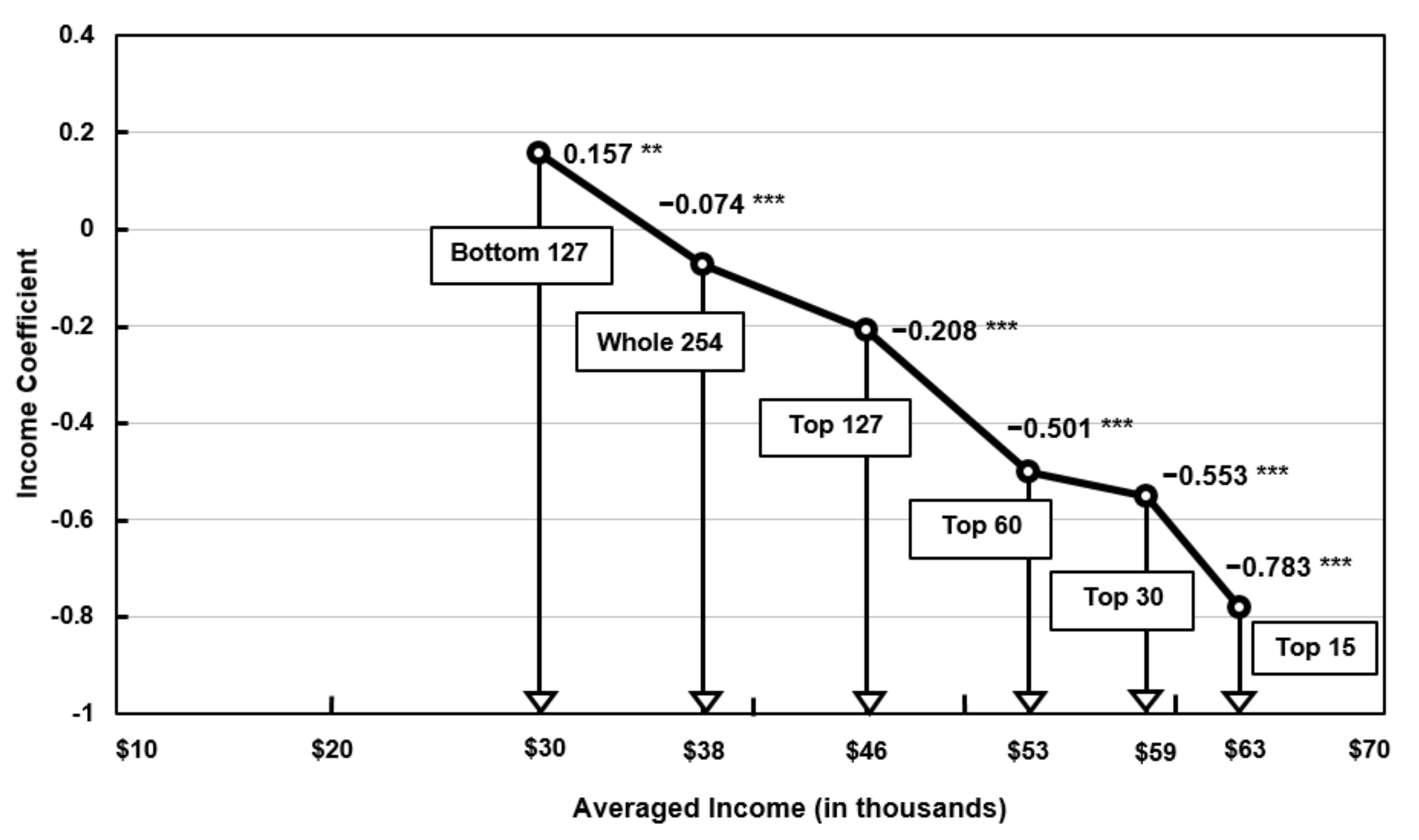
2.5 concentrations on the three separate groups of 254 cities by income, density, and population, and their respective five subgroups generated the following variable results. First, the full sample of 254 cities ranked by 2013 income per capita yielded a statistically significant −0.074. In other words, a 1% increase in income per capita generated a −0.074% reduction of PM2.5 concentrations, while the impact from the other factors of density and population size were held constant, as shown in Table 4.
When the subgroup of 254 cities was divided into the top 127 high-income cities, the income coefficient increased to −0.208, which was about 2.7 times larger than the income coefficient obtained from the 254 cities. A 1% increase in income per capita reduced PM2.5 concentrations by 0.208% for the subgroup of 127 high-income cities. In contrast, the sample of the remaining bottom 127 low-income cities yielded a statistically significant coefficient of +0.157, while the other factors held constant. Specifically, a 1% increase in income increased PM2.5 concentrations by 0.157%, which indicated an income scale disadvantage for the bottom 127 low-income cities. These results suggest that there are effects from the EKC curve on cities with different income levels.
Furthermore, the contrasting results from the top 127 and the bottom 127 cities suggested the possibility of an even greater income scale advantage for cities with very high income per capita. Therefore, extended STIRPAT analysis of income coefficients for the samples of the top 15, top 30, and top 60 high-income cities were examined. The result was that the top 60 cities yielded −0.505, while the top 30 yielded −0.582. Finally, the top 15 high-income cities generated the highest negative income coefficient of −0.783, which was about 10 times larger than the income coefficient of the 254 cites at −0.074, indicating the existence of a very large-scale advantage of income for PM2.5 pollution. Furthermore, all three income coefficients met the statistical test of significance.
In summary, a very large-scale advantage of income for reduced PM2.5 pollution was evident in the top 15, top 30, and top 60 high-income cities. This income scale advantage continued through the top 127 cities at a somewhat reduced scale. However, the scale advantage showed a slight scale disadvantage for the remaining bottom 127 cities with lower income per capita. The full sample of 254 cities showed a moderate yet statistically significant income scale advantage by combining different income coefficients from these city subgroups.
The same STIRPAT multivariate panel regression was applied first to the full sample of 254 cities, ranked by 2013 population density. The density coefficient from the full sample of 254 cities yielded statistically significant density coefficients of +0.058, as shown in Table 5, which resembled the results in a German study [14] with a density coefficient of +0.08. In other words, a 1% increase in density yielded a 0.058% increase in PM2.5 concentration, demonstrating that the impact of density on PM2.5 concentrations was positive. When the full sample of 254 cities was divided into the subsample of the top 127 cities with higher density, the density coefficient was more or less unchanged at 0.053, meeting the statistical test of significance, while the effects from the other factors held constant.
The bottom 127 cities with lower densities yielded a statistically significant density coefficient of +0.142, which was substantially higher than the density coefficients of both the top 127 and all 254 cities. In other words, the positive impact of population density on PM2.5 pollution was much greater for the group of cities with lower densities compared to the group of cities with higher densities.
The result for the top 60 cities yielded a statistically significant coefficient of +0.05, which was nearly the same as the +0.058 coefficient estimated for all 254 cities. Similarly, the density coefficients for the top 30 cities remained at +0.061. However, for the top 15 cities, the density coefficient more than doubled to +0.13. The density coefficients for the top 15 cities did not meet the statistical test of significance, whereas the density coefficient for the top 30 cities did.
In summary, all of the density coefficients displayed a positive impact of density on greater PM2.5 pollution. The positive impact was greater for the 127 cities with lower population densities over both the 127 cities with higher population densities, and the full sample of all 254 cites. The top 60 and 30 cities displayed density coefficients nearly equal to those of the top 127 cities and all 254 cities. However, the top 15 cities displayed a substantially higher density coefficient, approaching the density coefficient derived from the bottom 127 cities. In sum, the overall pattern of density coefficients followed a U-shaped pattern, providing an interesting contrast to the inverse U-shaped pattern of the EKC.
Finally, the full sample of 254 cities ranked by 2013 population size was subjected to the same panel regression analysis. The resulting population coefficient of −0.018 met the statistical test of significance. To explain, a 1% increase in population would reduce PM2.5 concentrations slightly by 0.018% for the full sample of 254 cities, while the effects of the other factors of income and density were held constant, as listed in Table 6. However, compared to the income and density coefficients estimated earlier, the magnitude of impact of population size is quite moderate. In addition, similar to the effect of income, larger population sizes implied a smaller reduction in PM2.5 concentrations.
To differentiate the degree of impact between large versus small population size, the full sample of 254 cities was again divided into the subgroups of the top 127 largest population cities and the remaining 127 smallest population cities. The resulting population coefficient for the top 127 cities was much smaller at −0.009, compared to the −0.018 estimated for all 254 cities, but the coefficient failed to meet the statistical test of significance. The remaining 127 cities with smaller populations yielded a substantially larger population coefficient of +0.024, which again did not meet the statistical test of significance.
To determine the impact of population mega cities of the top 15 most populated cities, the panel regression yielded a statistically significant population coefficient of +0.261. For the subgroup of the top 30 most populated cities, the population coefficient was substantially smaller at +0.027, but failed to meet the statistical test of significance. For the top 60 cites, the population coefficient yielded −0.034, indicating the same population impact on PM2.5 concentrations as the subgroups of the top 127 and all 254 cities. However, only the two population coefficients for the top 15 cities and all 254 cities met the statistical test of significance.
In sum, although an increasing population size for the full sample of 254 cities yielded a moderate reduction in PM2.5 pollution, the results from the subgroup analyses did not support such an impact. On the contrary, the subgroup of 15 mega cities indicated a much higher impact of increasing, not decreasing, PM2.5 pollution. The results from the remaining subgroups were inconclusive.
In order to verify the appropriateness of subgroups used in this study so far, the multivariate panel regression was replicated for the four additional subgroups for the respective independent variables. Specifically, we added the subgroups of the top 20, top 50, top 100, and top 200 cities. Table 7 shows the newly derived income, density, and population coefficients for the newly added four subgroups together with the coefficients estimated earlier for the five subgroups of the top 15, top 30, top 60, top 127, and bottom 127 cities.
The four newly estimated income coefficients, all of which are statistically significant, follow the overall declining pattern of coefficients from the top 15 to bottom 127 cities in perfect alignment, indicating the robustness of our previous estimation of the five subgroups. As for the four new density coefficients, they, in general, also support the overall “U” shaped pattern, with a wide flat bottom displayed by the previous five coefficients. The distribution of the four new population coefficients, also, support the overall pattern established by the previously estimated coefficients, where the top 15 displayed the highest coefficients. Similarly, the new coefficients from the subgroup of top 20 cities also displayed the highest coefficients among the new four subgroups.
Since both the top 127 largest cities and the bottom 127 smallest cities failed to generate statistically significant population coefficients, we used an alternative model of threshold regression as a robustness check. The results, shown in Table 8, indicated that the optimal single-threshold value was estimated at 0.768 million inhabitants. We divided the full sample of 254 cities into Region 1 with more than 0.768 million inhabitants and Region 2 with less than 0.768 million inhabitants. Region 1 with 94 cities had an average population size of 2,903,502 inhabitants and Region 2 with 160 cities had an averaged population size of 436,966 inhabitants.
The population coefficient for Region 1 generated a statistically significant +0.045, compared to −0.009 for the top 127 cities, whereas Region 2 generated a statistically insignificant +0.012, compared to +0.024 for the bottom 127 cities.
In sum, the robustness test with threshold regression using the subgroups of alternative population size for the top 94 cities and the bottom 160 cities improved the statistical validity for the subgroup of cities with large populations. However, the basic piecewise linear pattern of population coefficients remained essentially intact.

5. Conclusions

The key findings from this research can be summarized as follows. First, the impact of income measured by city GDP per capita on PM2.5 pollution for the full sample of 254 cities was highest, in that a 1% increase in income generated a −0.074 reduction of PM2.5 concentrations. In contrast, the impact of population density was nearly as high, in that a 1% increase in population density resulted in a 0.058% increase of PM2.5 concentrations. The impact from population size was quite modest, in that a 1% increase of population size resulted in a reduction of only 0.018%.
Second, when all 254 cities were categorized into five subgroups of the top 127, bottom 127, top 60, top 30, and top 15 cities, the impact of income, density, and population varied so widely that each influencing factor needed a separate in-depth analysis. We provide a summary in Table 9 of the six coefficients for each of the three influencing factors of income, density, and population. We also present the average values during the study period of income, density, and population for all 254 cities as well as for each of the respective five subgroups under analysis.
Third, the results of the income subgroup analysis showed the most consistent pattern following the EKC. The richest cities displayed the highest scale advantage for greater pollution reduction, whereas the lower income cities experienced a scale of diseconomy with pollution increases. To elaborate, Figure 1 shows that the income coefficient for the top 15 highest-income subgroup with an average income of $63,132 experienced a reduction of −0.783% in PM2.5 pollution, whereas the bottom 127 lower-income cities with an average income of $30,007 experienced a pollution increase of 0.157% for the same 1% increase in income.
To explain this pattern in the context of the EKC, many cities in the subgroup of cities with an average income of $30,007 had not reached the peak of their EKC, and thus, experienced increasing pollution as their income increased. In contrast, many cities in the subgroup with an average income of $45,537 had surpassed the peak, so experienced a win-win relation of increased income and reduced pollution. Cities with the highest income level experienced proportionately greater pollution reductions, as predicted by the EKC.
Fourth, the results of the density subgroup analysis showed a somewhat opposite pattern from the income subgroups. As shown in Figure 2, the bottom 127 low-density cites with an average density of 202 persons per km2 generated the highest density coefficient of +0.142, whereas the top 15 high-density cities also generated an equally high density coefficient of +0.119. In the remaining subgroups, the density coefficient clustered closely around the density coefficient derived from all 254 cities. Thus, the overall distribution of density coefficients resembled a U-shaped pattern, which is opposite to the inverse U-shaped EKC.
As noted in the earlier section of the literature review, many cities in the U.S and some European countries with low-density urban sprawl may have been responsible for the unusual high-density coefficient of +0.142 estimated for the subgroups of the bottom 127 cities. For example, the bottom 127 subgroup contained a large minority of 36 American cities. Furthermore, this subgroup contained 14 American cities in the bottom 20 lowest density cities, indicating the impact of low-density sprawl cities.
The high-density coefficient of 0.119 from the subgroup of the top 15 cities with a very high average density of 4010 inhabitants per km2 may reflect the fact that extremely high-density cities will begin to experience excessive spatial concentration and consequently increasing vehicle emissions due to severe congestion as well as the high number of people exposed to pollution. These can bring about a rapidly rising air pollution. Furthermore, the fact that there are seven high-density Japanese cities included in the top 15 subgroup may have generated another cause for the unusually high coefficient derived for this subgroup.
Fifth, the results from the population subgroups were somewhat inconsistent and contradictory in that only the full sample of 254 cities and the top 15 most populous mega cities generated statistically significant population coefficients. All 254 cities generated −0.018, while the top 15 subgroup generated +0.261. In other words, most cities would experience a very modest pollution reduction in the full sample of 254 cities, whereas the most populous cities in the top 15 subgroup would experience the largest increase in PM2.5 pollution. The population coefficient from the remaining subgroups clustered around the population density of the full sample of all cities group. Therefore, the distribution of population coefficients can be approximated using a piecewise linear relation, as displayed in Figure 3. In short, unlike the case of income and density, the population size of cities appears to not have a substantial impact on PM2.5 pollution. The only exception was in the case of the most populous 15 mega cities with an average population size around 10 million inhabitants.
It would be interesting to compare the results of this study to the results of studies on Chinese cities discussed earlier in the literature review section. First, the impact of income on PM2.5 pollution between the two groups was quite similar, as both the previous studies and our study verified the theory of EKC. One difference may be that the inflection point of the EKC in China could be somewhat lower in the range of $9186 to $18,506 per capita [8]. In comparison, the average income for the bottom 127 cities in this study, generating a positive income coefficient, was estimated at $30,007. Another difference may relate to the very large-scale economy estimated for the top 15 high-income subgroup in this study, which may be different in high-income Chinese cities.
As for population density, both groups of studies verified the result of increasing pollution as a function of increasing population density. However, the U-shaped distribution of density coefficients revealed in this study may be due to many low-density urban sprawls found particularly in the U.S. For example, the average density for all 254 cities was quite low (i.e., estimated at 704 persons per km2). In comparison, the average population density for 285 cities in China during a similar study period of 2001 to 2012 was estimated at a much higher density of 1149.86 persons per km2 [4]. Finally, both groups of studies found that the impact of population size on PM2.5 pollution was inconclusive, although our study revealed rapidly increasing pollution from the most populous cities with an average of 10 million inhabitants.
The findings of this study have policy implications for all countries. An ideal combination of the three influencing factors examined in this study that are most favorable to pollution reduction are (1) an average income per capita of $38,000 or more; (2) population density in the range of 1000 to 2000 population per km2; and (3) a medium population size between 1.5 million to 4 million inhabitants. In contrast, the worst combination of the three factors are (1) low-income cities with significantly less than $30,000 per capita; (2) the highest population density of more than 4000 persons per km2; and (3) the largest population size of more than 10 million inhabitants.
We realize, however, that such an ideal combination would be quite difficult to achieve in most cities. Fortunately, the results of this study have identified a rather wide indifference zone of the average values in all three factors. For the income, any city income per capita over $38,000 would generate a substantial pollution reduction. For density, the wide indifference zone ranges from about 700 to 3000 persons per km2, while the indifference zone of population size ranges from 1.3 million to 6.4 million inhabitants.
There are several limitations to this study that represent possible topics for future studies. One major limitation is the omission of several socio-economic factors related to PM2.5 pollution that have been analyzed in previous studies. For example, several previous studies on Chinese cities have included other influencing factors such as industrial structure, traffic intensity, energy and electricity usage, and coal consumption [2,3,4,7]. Another group of omitted factors include meteorological elements such as temperature, precipitation, wind, and humidity [9]. Other omitted variables may include atmospheric chemistry and the long-distance transport of pollution [9,62,63,64,65,66]. These omitted variables could be included in future studies, and thus could revise the interactions related to socio-economic factors examined in this study. In other words, we have provided some evidence for the robust association between the factors of income, density, and population to PM2.5 pollutions, rather than evidence of causality. Thus, future work should continue to establish the causal relationships to control air pollutions.
Despite these limitations, this research revealed the role of high-income cities in developed countries and added insights about how pollution reduction can have a greater impact compared to developing countries such as China. This study also supports the positive impact of high population density cities on increasing pollution, which is also the case in developing countries. Going beyond this basic notion, this study proposes a U-shaped pattern of density coefficients as a function of variable population densities of cities for developed countries.

Author Contributions

Conceptualization, methodology, and analysis, Y.-S.C. and S.-M.K.; original draft preparation, Y.-S.C. and M.-J.K.; review and editing, Y.-S.C., M.-J.K., and S.-M.K. All authors have read and agreed to the published version of the manuscript.

Funding

This research received no external funding.

Institutional Review Board Statement

Not applicable.

Informed Consent Statement

Not applicable.

Data Availability Statement

Data sources are reported in our Method and Data section. Data are available from these sources.

Conflicts of Interest

The authors declare no conflict of interest.

Appendix A

Table A1. Ranking of 254 cities into 5 subgroups by income per capita.
RankCitiesgdp/capPopulationDensityPM2.5
1USA: San Francisco (Greater)84,921 6,457,022 128511
2USA: Boston73,186 4,276,297 23438
3USA: Houston72,001 6,422,530 2859
4USA: New York (Greater)70,399 20,000,933 175710
5USA: New Haven69,899 1,807,423 106810
6DE: Ingolstadt68,518 463,060 17118
7USA: Washington (Greater)68,073 8,794,922 56110
8USA: Hartford64,337 1,216,966 5859
9USA: Philadelphia (Greater)61,836 6,407,666 75610
10DE: Dusseldorf61,698 1,511,967 170814
11USA: Minneapolis61,415 3,405,918 23810
12USA: Portland61,332 2,209,459 2016
13FR: Paris61,301 11,866,785 118617
14USA: Dallas60,787 6,980,428 27210
Top 15USA: Denver60,7522,696,3082268
16USA: Indianapolis60,360 1,938,160 23211
17DE: Frankfurt am Main60,351 2,544,366 64815
18USA: Tulsa59,447 1,002,698 5910
19USA: Milwaukee58,426 1,571,740 48510
20USA: Chicago 58,099 9,548,402 108911
21USA: Nashville 58,031 294,618 42710
22USA: New Orleans56,524 1,219,579 1508
23DE: Stuttgart56,386 2,648,143 80216
24UK: London55,954 11,544,026 289715
25DE: Heilbronn55,901 441,943 40217
26USA: East Baton Rouge55,885 819,304 8410
27USA: Austin55,841 1,894,164 2578
28USA: Charlotte55,486 1,839,138 3439
29USA: Columbus55,401 1,935,123 19212
Top 30UK: Aberdeen54,812484,840776
31USA: Cincinnati54,682 2,084,836 26811
32USA: Atlanta52,745 5,183,715 46510
33DE: Hamburg52,487 3,143,783 48711
34USA: Jackson (MO)52,441 1,977,173 1249
35USA: Richmond (Greater)51,870 1,112,531 1019
36DE: Bonn51,515 889,551 79713
37USA: Salt Lake51,295 1,539,116 549
38DE: Karlsruhe51,240 722,801 66716
39DE: Wiesbaden51,140 453,599 55914
40USA: Pittsburgh50,378 1,441,884 64611
41USA: Oklahoma50,025 1,281,128 1209
42DE: Regensburg50,009 436,621 17818
43DE: Mainz49,981 405,874 67115
44USA: Lancaster (NE)49,898 328,854 11011
45USA: St. Louis49,457 2,596,184 23710
46DE: Mannheim-Ludwigshafen49,358 1,145,686 66116
47DE: Muenster49,276 512,138 46112
48UK: Guildford49,131 263,440 76412
49USA: Detroit (Greater)48,811 4,360,382 88511
50DE: Koblenz48,496 319,944 39213
51DE: Braunschweig-Salzgitter Wolfsburg48,491 977,157 27913
52USA: Memphis47,895 1,302,172 14610
53DE: Ulm47,753 470,839 26316
54DE: Darmstadt46,621 434,462 66116
55ES: Vitoria46,600 264,719 20010
56USA: Virginia Beach46,383 1,165,789 2869
57USA: Rochester (NY)46,221 857,051 32010
58USA: Albany45,650 976,721 1188
59FR: Lyon45,114 1,958,191 62217
Top 60USA: Sacramento44,6802,213,56447811
61DE: Hannover44,588 1,267,062 45812
62DE: Schweinfurt44,541 267,890 13616
63JPN: Toyohashi44,353 665,226 96114
64UK: Oxford44,033 527,670 28113
65USA: Erie (NY)43,694 1,136,993 82311
66DE: Aschaffenburg43,603 368,348 26116
67USA: Charleston43,545 711,407 1529
68USA: Tuscaloosa43,490 244,054 4311
69USA: Montgomery (OH)43,485 697,435 64611
70USA: Phoenix43,099 4,390,565 31512
71USA: Lafayette43,007 427,049 5412
72DE: Reutlingen42,986 273,578 27216
73UK: Edinburgh42,842 849,720 5829
74USA: Miami (Greater)42,808 6,014,211 34137
75JPN: Tokyo42,785 35,221,137 863516
76USA: Providence42,772 969,960 9809
77USA: Roanoke42,757 311,993 658
78ES: Barcelona42,739 4,019,011 207614
79FR: Toulouse42,275 1,277,646 26712
80DE: Offenburg42,147 412,179 23215
81ES: Madrid42,105 6,379,915 99110
82DE: Bremen42,075 1,230,691 22112
83JPN: Toyota41,974 8,498,701 240313
84USA: Allen41,952 396,450 45310
85DE: Heidelberg41,759 677,291 63916
86USA: San Antonio41,750 2,298,261 1228
87USA: Las Vegas41,274 2,074,253 287
88DE: Wurzburg41,216 497,551 16816
89UK: Bristol40,865 913,519 104814
90DE: Kassel40,851 427,403 33114
91DE: Saarbrucken40,635 800,458 58614
92USA: Hamilton (TN)40,424 542,036 13411
93UK: Cambridge40,261 360,154 23213
94DE: Augsburg40,217 639,038 34517
95JPN: Hamamatsu40,014 957,085 68113
96DE: Freiburg im Breisgau39,783 623,036 30315
97JPN: Kanazawa39,658 684,018 72213
98USA: Jacksonville39,619 1,485,547 1329
99JPN: Fujieda39,605 457,650 106914
100JPN: Numazu39,600 553,358 110013
101DE: Iserlohn39,246 420,986 45112
102JPN: Yokkaichi38,989 1,058,231 114514
103DE: Pforzheim38,695 307,352 53615
104USA: Albuquerque38,603 929,424 287
105USA: Knox38,534 463,248 7239
106DE: Aachen38,469 539,521 99513
107ES: Pamplona38,280 362,229 24111
108JPN: Utsunomiya38,171 882,046 64614
109DE: Siegen38,160 405,088 24412
110DE: Osnabruck38,113 506,726 23912
111DE: Paderborn37,865 298,853 28112
112DE: Rosenheim37,486 307,074 21318
113USA: Spokane37,376 501,584 518
114UK: Southampton37,211 664,608 48113
115JPN: Toyama37,118 593,754 82812
116FR: Nice36,979 824,441 35316
117DE: Kiel36,979 632,735 19510
118ES: Bilbao36,936 1,033,172 77011
119JPN: Fukui36,794 547,512 30614
120JPN: Morioka36,463 413,105 17810
121FR: Nantes36,454 915,985 34813
122FR: Dijon36,390 402,912 11115
123JPN: Mito36,331 703,770 68114
124DE: Berlin36,248 4,950,913 30214
125DE: Oldenburg (Oldenburg)36,096 402,152 22411
126JPN: Sendai36,011 1,464,672 143513
Top 127FR: Rennes35,966701,15321913
128FR: Reims35,964 320,879 13715
129USA: Tallahassee35,883 373,212 819
130FR: Strasbourg35,874 771,559 44916
131JPN: Hitachi35,740 316,365 42013
132UK: Northampton35,711 457,540 31313
133DE: Gottingen35,692 383,137 16914
134JPN: Tokushima35,601 569,456 62015
135DE: Wetzlar35,552 251,578 25513
136JPN: Hiroshima35,436 1,432,615 314917
137FR: Bordeaux35,367 1,174,012 23512
138USA: Fresno (Greater)35,140 1,105,606 19815
139JPN: Kurashiki34,908 1,516,388 96216
140JPN: Takamatsu34,900 562,614 128515
141FR: Pau34,751 267,702 14611
142FR: Orleans34,633 424,619 16414
143FR: Clermont-Ferrand34,545 476,713 20213
144JPN: Niigata34,529 805,385 144614
145ES: Palma de Mallorca34,502 643,352 35511
146JPN: Wakayama34,473 541,730 118015
147DE: Lubeck34,352 407,813 29511
148FR: Rouen34,337 689,626 31316
149JPN: Kofu34,222 586,614 43312
150JPN: Kurume34,202 409,982 189819
151FR: Grenoble34,031 661,221 28216
152JPN: Nagano33,981 572,858 73212
153DE: Flensburg33,897 274,656 1389
154UK: Derby33,806 472,015 78314
155JPN: Koriyama33,754 518,284 51312
156UK: Manchester33,644 3,246,448 176213
157DE: Leipzig33,626 978,997 26615
158JPN: Matsumoto33,581 426,101 47711
159JPN: Fukushima33,569 449,041 54812
160DE: Erfurt33,561 519,509 20115
161USA: Montgomery (AL)33,516 451,815 3911
162FR: Le Havre33,328 297,916 53716
163USA: Lubbock33,053 351,009 296
164DE: Trier33,037 248,567 22713
165DE: Halle an der Saale33,026 420,210 29214
166DE: Magdeburg33,017 496,349 12514
167UK: Brighton and Hove32,843 440,222 150216
168JPN: Kitakyushu32,749 1,332,183 268020
169UK: Glasgow32,740 1,790,510 78010
170JPN: Oita32,635 732,952 56817
171JPN: Fukuoka32,630 2,680,715 591821
172DE: Rostock32,549 412,399 12111
173JPN: Matsuyama32,249 625,918 613717
174FR: Caen32,169 434,109 21114
175FR: Valenciennes32,133 358,729 68716
176FR: Avignon32,098 318,245 50513
177JPN: Asahikawa32,090 388,628 2329
178FR: Annecy32,023 272,588 25615
179UK: Ipswich31,738 349,520 23513
180FR: Tours31,733 460,093 18314
181FR: Lille31,700 1,366,909 164716
182FR: Poitiers31,591 266,275 11813
183FR: Montpellier31,425 668,380 37212
184JPN: Obihiro31,404 262,830 1509
185DE: Dresden31,378 1,327,534 24116
186JPN: Himeji31,342 720,892 113916
187FR: Le Mans31,328 355,467 17115
188JPN: Sapporo31,201 2,192,770 162911
189UK: Leicester31,141 849,964 72813
190ES: Valladolid30,983 414,196 4318
191UK: Leeds30,926 2,550,810 74012
192JPN: Yamagata30,785 422,839 57113
193UK: Norwich30,726 388,299 26612
194DE: Kaiserslautern30,696 273,554 22614
195DE: Bremerhaven30,604 307,055 14911
196JPN: Aomori30,530 309,601 58511
197FR: Nancy30,446 474,407 17614
198FR: Dunkerque30,390 273,513 42517
199JPN: Hakodate30,317 345,811 56210
200JPN: Hachinohe30,196 324,182 40510
201USA: El Paso (TX)30,194 833,522 708
202JPN: Akita30,093 399,793 62413
203JPN: Miyazaki29,868 493,598 63915
204JPN: Kumamoto29,811 1,130,440 75320
205FR: Amiens29,772 309,154 14517
206DE: Zwickau29,645 329,603 39015
207UK: Nottingham29,576 884,410 106813
208UK: Dundee City29,547 264,390 1218
209FR: Mulhouse29,505 407,282 41416
210FR: Angers29,380 406,872 22714
211DE: Hildesheim29,355 276,440 24812
212FR: Besancon29,345 270,164 13815
213JPN: Nagasaki29,342 641,205 186917
214UK: Liverpool29,312 1,178,689 620413
215DE: Schwerin29,287 303,031 6411
216JPN: Kagoshima29,173 715,775 147315
217FR: Limoges29,160 307,992 11412
218FR: Brest29,048 365,055 33610
219FR: Saint-Etienne28,911 526,369 42513
220UK: Plymouth28,849 396,686 19311
221UK: Exeter28,828 460,870 19211
222UK: Blackburn with Darwen28,709 285,594 48910
223UK: Newcastle upon Tyne28,450 1,152,859 2309
224ES: Oviedo28,336 304,133 4078
225JPN: Kochi28,335 513,465 34216
226ES: Valencia28,298 1,663,496 124312
227ES: Santander27,833 372,909 6089
228DE: Neubrandenburg27,794 278,044 4812
229UK: Cardiff27,691 767,542 109513
230ES: Santa Cruz de Tenerife27,235 492,820 131112
231DE: Gorlitz27,186 264,402 13017
232FR: Metz27,067 368,383 24714
233UK: Kingston upon Hull26,879 593,260 24611
234UK: Lincoln26,721 296,097 14311
235UK: Stoke-on-Trent26,405 472,866 82211
236UK: Sheffield26,220 1,154,133 419712
237UK: Blackpool26,076 326,318 196613
238ES: Murcia26,062 591,669 199211
239UK: Middlesbrough25,983 467,304 190711
240UK: Swansea25,891 379,975 85812
241JPN: Naha25,838 1,170,320 37158
242FR: Toulon25,681 553,594 81813
243UK: Colchester25,622 317,030 93214
244ES: Gijon25,587 296,163 8639
245ES: Las Palmas25,354 620,841 112713
246ES: Vigo25,251 533,676 4309
247ES: Elche/Elx25,221 249,200 422412
248FR: Perpignan25,092 389,016 32611
249FR: Nimes24,987 338,177 41411
250ES: Seville24,789 1,498,774 37213
251ES: Alicante23,321 439,642 389112
252ES: Marbella23,226 285,326 50913
253ES: Granada22,719 538,657 40211
Bottom 127ES: Cordoba22,057355,03857711
Table A2. Ranking of 254 cities into 5 subgroups by population density.
RankCitiesDensitygdp/CapitaPopulationPM2.5
1 JPN01: Tokyo8635 42,785 35,221,137 16
2 UK006: Liverpool6204 29,312 1,178,689 13
3 JPN25: Matsuyama6137 32,249 625,918 17
4 JPN04: Fukuoka5918 32,630 2,680,715 21
5 ES505: Elche/Elx4224 25,221 249,200 12
6 UK010: Sheffield4197 26,220 1,154,133 12
7 ES021: Alicante3891 23,321 439,642 12
8 JPN10: Naha3715 25,838 1,170,320 8
9 USA09: Miami (Greater)3413 42,808 6,014,211 7
10 JPN08: Hiroshima3149 35,436 1,432,615 17
11 UK001: London2897 55,954 11,544,026 15
12 JPN09: Kitakyushu2680 32,749 1,332,183 20
13 JPN03: Toyota2403 41,974 8,498,701 13
14 USA11: Boston2343 73,186 4,276,297 8
Top 15ES002: Barcelona207642,7394,019,01114
16 ES007: Murcia1992 26,062 591,669 11
17 UK553: Blackpool1966 26,076 326,318 13
18 UK559: Middlesbrough1907 25,983 467,304 11
19 JPN42: Kurume1898 34,202 409,982 19
20 JPN24: Nagasaki1869 29,342 641,205 17
21 UK008: Manchester1762 33,644 3,246,448 13
22 USA01: New York (Greater)1757 70,399 20,000,933 10
23 DE011: Dusseldorf1708 61,698 1,511,967 14
24 FR009: Lille1647 31,700 1,366,909 16
25 JPN05: Sapporo1629 31,201 2,192,770 11
26 UK515: Brighton and Hove1502 32,843 440,222 16
27 JPN19: Kagoshima1473 29,173 715,775 15
28 JPN15: Niigata1446 34,529 805,385 14
29 JPN06: Sendai1435 36,011 1,464,672 13
Top 30ES025: Santa Cruz de Tenerife131127,235492,82012
31 USA05: San Francisco (Greater)1285 84,921 6,457,022 11
32 JPN28: Takamatsu1285 34,900 562,614 15
33 ES003: Valencia1243 28,298 1,663,496 12
34 FR001: Paris1186 61,301 11,866,785 17
35 JPN33: Wakayama1180 34,473 541,730 15
36 JPN12: Yokkaichi1145 38,989 1,058,231 14
37 JPN20: Himeji1139 31,342 720,892 16
38 ES008: Las Palmas1127 25,354 620,841 13
39 JPN31: Numazu1100 39,600 553,358 13
40 UK009: Cardiff1095 27,691 767,542 13
41 USA03: Chicago 1089 58,099 9,548,402 11
42 JPN38: Fujieda1069 39,605 457,650 14
43 USA27: New Haven1068 69,899 1,807,423 10
44 UK029: Nottingham1068 29,576 884,410 13
45 UK011: Bristol1048 40,865 913,519 14
46 DE507: Aachen995 38,469 539,521 13
47 ES001: Madrid991 42,105 6,379,915 10
48 USA53: Providence980 42,772 969,960 9
49 JPN07: Kurashiki962 34,908 1,516,388 16
50 JPN23: Toyohashi961 44,353 665,226 14
51 UK546: Colchester932 25,622 317,030 14
52 USA13: Detroit (Greater)885 48,811 4,360,382 11
53 ES023: Gijon863 25,587 296,163 9
54 UK517: Swansea858 25,891 379,975 12
55 JPN26: Toyama828 37,118 593,754 12
56 USA44: Erie (NY)823 43,694 1,136,993 11
57 UK027: Stoke-on-Trent822 26,405 472,866 11
58 FR032: Toulon818 25,681 553,594 13
59 DE007: Stuttgart802 56,386 2,648,143 16
Top 60DE034: Bonn79751,515889,55113
61 UK518: Derby783 33,806 472,015 14
62 UK004: Glasgow780 32,740 1,790,510 10
63 ES019: Bilbao770 36,936 1,033,172 11
64 UK033: Guildford764 49,131 263,440 12
65 USA06: Philadelphia (Greater)756 61,836 6,407,666 10
66 JPN11: Kumamoto753 29,811 1,130,440 20
67 UK003: Leeds740 30,926 2,550,810 12
68 JPN29: Nagano732 33,981 572,858 12
69 UK014: Leicester728 31,141 849,964 13
70 USA97: Knox723 38,534 463,248 9
71 JPN17: Kanazawa722 39,658 684,018 13
72 FR034: Valenciennes687 32,133 358,729 16
73 JPN14: Hamamatsu681 40,014 957,085 13
74 JPN21: Mito681 36,331 703,770 14
75 DE037: Mainz671 49,981 405,874 15
76 DE035: Karlsruhe667 51,240 722,801 16
77 DE084: Mannheim-Ludwigshafen661 49,358 1,145,686 16
78 DE025: Darmstadt661 46,621 434,462 16
79 DE005: Frankfurt am Main648 60,351 2,544,366 15
80 USA41: Pittsburgh646 50,378 1,441,884 11
81 JPN16: Utsunomiya646 38,171 882,046 14
82 USA66: Montgomery (OH)646 43,485 697,435 11
83 DE522: Heidelberg639 41,759 677,291 16
84 JPN36: Miyazaki639 29,868 493,598 15
85 JPN43: Akita624 30,093 399,793 13
86 FR003: Lyon622 45,114 1,958,191 17
87 JPN30: Tokushima620 35,601 569,456 15
88 ES015: Santander608 27,833 372,909 9
89 DE040: Saarbrucken586 40,635 800,458 14
90 USA40: Hartford585 64,337 1,216,966 9
91 JPN51: Aomori585 30,530 309,601 11
92 UK007: Edinburgh582 42,842 849,720 9
93 ES020: Cordoba577 22,057 355,038 11
94 JPN41: Yamagata571 30,785 422,839 13
95 JPN18: Oita568 32,635 732,952 17
96 JPN48: Hakodate562 30,317 345,811 10
97 USA04: Washington (Greater)561 68,073 8,794,922 10
98 DE020: Wiesbaden559 51,140 453,599 14
99 JPN39: Fukushima548 33,569 449,041 12
100 FR012: Le Havre537 33,328 297,916 16
101 DE533: Pforzheim536 38,695 307,352 15
102 JPN34: Koriyama513 33,754 518,284 12
103 ES533: Marbella509 23,226 285,326 13
104 FR039: Avignon505 32,098 318,245 13
105 UK557: Blackburn with Darwen489 28,709 285,594 10
106 DE002: Hamburg487 52,487 3,143,783 11
107 USA32: Milwaukee485 58,426 1,571,740 10
108 UK520: Southampton481 37,211 664,608 13
109 USA29: Sacramento478 44,680 2,213,564 11
110 JPN40: Matsumoto477 33,581 426,101 11
111 USA10: Atlanta465 52,745 5,183,715 10
112 DE504: Muenster461 49,276 512,138 12
113 DE013: Hannover458 44,588 1,267,062 12
114 USA116: Allen453 41,952 396,450 10
115 DE045: Iserlohn451 39,246 420,986 12
116 FR006: Strasbourg449 35,874 771,559 16
117 JPN27: Kofu433 34,222 586,614 12
118 ES009: Valladolid431 30,983 414,196 8
119 ES022: Vigo430 25,251 533,676 9
120 USA145: Nashville 427 58,031 294,618 10
121 FR011: Saint-Etienne425 28,911 526,369 13
122 FR042: Dunkerque425 30,390 273,513 17
123 JPN50: Hitachi420 35,740 316,365 13
124 FR040: Mulhouse414 29,505 407,282 16
125 FR044: Nimes414 24,987 338,177 11
126 ES013: Oviedo407 28,336 304,133 8
Top 127JPN49: Hachinohe40530,196324,18210
128 ES501: Granada402 22,719 538,657 11
129 DE529: Heilbronn402 55,901 441,943 17
130 DE042: Koblenz392 48,496 319,944 13
131 DE544: Zwickau390 29,645 329,603 15
132 ES004: Seville372 24,789 1,498,774 13
133 FR010: Montpellier372 31,425 668,380 12
134 ES010: Palma de Mallorca355 34,502 643,352 11
135 FR205: Nice353 36,979 824,441 16
136 FR008: Nantes348 36,454 915,985 13
137 DE033: Augsburg345 40,217 639,038 17
138 USA28: Charlotte343 55,486 1,839,138 9
139 JPN35: Kochi342 28,335 513,465 16
140 FR037: Brest336 29,048 365,055 10
141 DE513: Kassel331 40,851 427,403 14
142 FR043: Perpignan326 25,092 389,016 11
143 USA56: Rochester (NY)320 46,221 857,051 10
144 USA12: Phoenix315 43,099 4,390,565 12
145 FR215: Rouen313 34,337 689,626 16
146 UK528: Northampton313 35,711 457,540 13
147 JPN32: Fukui306 36,794 547,512 14
148 DE027: Freiburg im Breisgau303 39,783 623,036 15
149 DE001: Berlin302 36,248 4,950,913 14
150 DE510: Lubeck295 34,352 407,813 11
151 DE018: Halle an der Saale292 33,026 420,210 14
152 USA43: Virginia Beach286 46,383 1,165,789 9
153 USA08: Houston285 72,001 6,422,530 9
154 FR026: Grenoble282 34,031 661,221 16
155 UK560: Oxford281 44,033 527,670 13
156 DE523: Paderborn281 37,865 298,853 12
157 DE083: Braunschweig-Salzgitter Wolfsburg279 48,491 977,157 13
158 USA07: Dallas272 60,787 6,980,428 10
159 DE537: Reutlingen272 42,986 273,578 16
160 USA21: Cincinnati268 54,682 2,084,836 11
161 FR004: Toulouse267 42,275 1,277,646 12
162 DE008: Leipzig266 33,626 978,997 15
163 UK566: Norwich266 30,726 388,299 12
164 DE532: Ulm263 47,753 470,839 16
165 DE061: Aschaffenburg261 43,603 368,348 16
166 USA30: Austin257 55,841 1,894,164 8
167 FR048: Annecy256 32,023 272,588 15
168 DE079: Wetzlar255 35,552 251,578 13
169 DE542: Hildesheim248 29,355 276,440 12
170 FR017: Metz247 27,067 368,383 14
171 UK026: Kingston upon Hull246 26,879 593,260 11
172 DE540: Siegen244 38,160 405,088 12
173 DE009: Dresden241 31,378 1,327,534 16
174 ES014: Pamplona241 38,280 362,229 11
175 DE517: Osnabruck239 38,113 506,726 12
176 USA15: Minneapolis238 61,415 3,405,918 10
177 USA17: St. Louis237 49,457 2,596,184 10
178 FR007: Bordeaux235 35,367 1,174,012 12
179 UK569: Ipswich235 31,738 349,520 13
180 USA25: Indianapolis232 60,360 1,938,160 11
181 DE073: Offenburg232 42,147 412,179 15
182 JPN44: Asahikawa232 32,090 388,628 9
183 UK017: Cambridge232 40,261 360,154 13
184 UK013: Newcastle upon Tyne230 28,450 1,152,859 9
185 FR036: Angers227 29,380 406,872 14
186 DE026: Trier227 33,037 248,567 13
187 USA18: Denver226 60,752 2,696,308 8
188 DE044: Kaiserslautern226 30,696 273,554 14
189 DE520: Oldenburg (Oldenburg)224 36,096 402,152 11
190 DE012: Bremen221 42,075 1,230,691 12
191 FR013: Rennes219 35,966 701,153 13
192 DE069: Rosenheim213 37,486 307,074 18
193 FR023: Caen211 32,169 434,109 14
194 FR022: Clermont-Ferrand202 34,545 476,713 13
195 USA20: Portland201 61,332 2,209,459 6
196 DE032: Erfurt201 33,561 519,509 15
197 ES012: Vitoria200 46,600 264,719 10
198 USA45: Fresno (Greater)198 35,140 1,105,606 15
199 DE039: Kiel195 36,979 632,735 10
200 UK516: Plymouth193 28,849 396,686 11
201 USA31: Columbus192 55,401 1,935,123 12
202 UK018: Exeter192 28,828 460,870 11
203 FR035: Tours183 31,733 460,093 14
204 DE028: Regensburg178 50,009 436,621 18
205 JPN37: Morioka178 36,463 413,105 10
206 FR016: Nancy176 30,446 474,407 14
207 DE534: Ingolstadt171 68,518 463,060 18
208 FR038: Le Mans171 31,328 355,467 15
209 DE021: Gottingen169 35,692 383,137 14
210 DE524: Wurzburg168 41,216 497,551 16
211 FR019: Orleans164 34,633 424,619 14
212 USA69: Charleston152 43,545 711,407 9
213 USA42: New Orleans150 56,524 1,219,579 8
214 JPN53: Obihiro150 31,404 262,830 9
215 DE527: Bremerhaven149 30,604 307,055 11
216 USA37: Memphis146 47,895 1,302,172 10
217 FR045: Pau146 34,751 267,702 11
218 FR014: Amiens145 29,772 309,154 17
219 UK019: Lincoln143 26,721 296,097 11
220 DE052: Flensburg138 33,897 274,656 9
221 FR025: Besancon138 29,345 270,164 15
222 FR018: Reims137 35,964 320,879 15
223 DE077: Schweinfurt136 44,541 267,890 16
224 USA83: Hamilton (TN)134 40,424 542,036 11
225 USA33: Jacksonville132 39,619 1,485,547 9
226 DE074: Gorlitz130 27,186 264,402 17
227 DE019: Magdeburg125 33,017 496,349 14
228 USA24: Jackson (MO)124 52,441 1,977,173 9
229 USA19: San Antonio122 41,750 2,298,261 8
230 DE043: Rostock121 32,549 412,399 11
231 UK550: Dundee City121 29,547 264,390 8
232 USA39: Oklahoma120 50,025 1,281,128 9
233 USA52: Albany118 45,650 976,721 8
234 FR021: Poitiers118 31,591 266,275 13
235 FR024: Limoges114 29,160 307,992 12
236 FR020: Dijon111 36,390 402,912 15
237 USA132: Lancaster (NE)110 49,898 328,854 11
238 USA46: Richmond (Greater)101 51,870 1,112,531 9
239 USA60: East Baton Rouge84 55,885 819,304 10
240 USA119: Tallahassee81 35,883 373,212 9
241 UK016: Aberdeen77 54,812 484,840 6
242 USA59: El Paso (TX)70 30,194 833,522 8
243 USA135: Roanoke65 42,757 311,993 8
244 DE031: Schwerin64 29,287 303,031 11
245 USA51: Tulsa59 59,447 1,002,698 10
246 USA34: Salt Lake54 51,295 1,539,116 9
247 USA108: Lafayette54 43,007 427,049 12
248 USA89: Spokane51 37,376 501,584 8
249 DE064: Neubrandenburg48 27,794 278,044 12
250 USA162: Tuscaloosa43 43,490 244,054 11
251 USA96: Montgomery (AL)39 33,516 451,815 11
252 USA126: Lubbock29 33,053 351,009 6
253 USA22: Las Vegas28 41,274 2,074,253 7
Bottom 127USA54: Albuquerque2838,603929,4247
Table A3. Ranking of 254 cities into 5 subgroups by population.
RankCitiesPopulationDensitygdp/CapitaPM2.5
1JPN: Tokyo35,221,137 8635 42,785 16
2USA: New York (Greater)20,000,933 1757 70,399 10
3FR: Paris11,866,785 1186 61,301 17
4UK: London11,544,026 2897 55,954 15
5USA: Chicago 9,548,402 1089 58,099 11
6USA: Washington (Greater) 8,794,922 561 68,073 10
7JPN: Toyota 8,498,701 2403 41,974 13
8USA: Dallas 6,980,428 272 60,787 10
9USA: San Francisco (Greater) 6,457,022 1285 84,921 11
10USA: Houston 6,422,530 285 72,001 9
11USA: Philadelphia (Greater) 6,407,666 756 61,836 10
12ES: Madrid 6,379,915 991 42,105 10
13USA: Miami (Greater) 6,014,211 3413 42,808 7
14USA: Atlanta 5,183,715 465 52,745 10
Top 15DE: Berlin4,950,91330236,24814
16USA: Phoenix 4,390,565 315 43,099 12
17USA: Detroit (Greater) 4,360,382 885 48,811 11
18USA: Boston 4,276,297 2343 73,186 8
19ES: Barcelona 4,019,011 2076 42,739 14
20USA: Minneapolis 3,405,918 238 61,415 10
21UK: Manchester 3,246,448 1762 33,644 13
22DE: Hamburg 3,143,783 487 52,487 11
23USA: Denver 2,696,308 226 60,752 8
24JPN: Fukuoka 2,680,715 5918 32,630 21
25DE: Stuttgart 2,648,143 802 56,386 16
26USA: St. Louis 2,596,184 237 49,457 10
27UK: Leeds 2,550,810 740 30,926 12
28DE: Frankfurt am Main 2,544,366 648 60,351 15
29USA: San Antonio 2,298,261 122 41,750 8
Top 30USA: Sacramento2,213,56447844,68011
31USA: Portland 2,209,459 201 61,332 6
32JPN: Sapporo 2,192,770 1629 31,201 11
33USA: Cincinnati 2,084,836 268 54,682 11
34USA: Las Vegas 2,074,253 28 41,274 7
35USA: Jackson (MO) 1,977,173 124 52,441 9
36FR: Lyon 1,958,191 622 45,114 17
37USA: Indianapolis 1,938,160 232 60,360 11
38USA: Columbus 1,935,123 192 55,401 12
39USA: Austin 1,894,164 257 55,841 8
40USA: Charlotte 1,839,138 343 55,486 9
41USA: New Haven 1,807,423 1068 69,899 10
42UK: Glasgow 1,790,510 780 32,740 10
43ES: Valencia 1,663,496 1243 28,298 12
44USA: Milwaukee 1,571,740 485 58,426 10
45USA: Salt Lake 1,539,116 54 51,295 9
46JPN: Kurashiki 1,516,388 962 34,908 16
47DE: Dusseldorf 1,511,967 1708 61,698 14
48ES: Seville 1,498,774 372 24,789 13
49USA: Jacksonville 1,485,547 132 39,619 9
50JPN: Sendai 1,464,672 1435 36,011 13
51USA: Pittsburgh 1,441,884 646 50,378 11
52JPN: Hiroshima 1,432,615 3149 35,436 17
53FR: Lille 1,366,909 1647 31,700 16
54JPN: Kitakyushu 1,332,183 2680 32,749 20
55DE: Dresden 1,327,534 241 31,378 16
56USA: Memphis 1,302,172 146 47,895 10
57USA: Oklahoma 1,281,128 120 50,025 9
58FR: Toulouse 1,277,646 267 42,275 12
59DE: Hannover 1,267,062 458 44,588 12
Top 60DE: Bremen1,230,69122142,07512
61USA: New Orleans 1,219,579 150 56,524 8
62USA: Hartford 1,216,966 585 64,337 9
63UK: Liverpool 1,178,689 6204 29,312 13
64FR: Bordeaux 1,174,012 235 35,367 12
65JPN: Naha 1,170,320 3715 25,838 8
66USA: Virginia Beach 1,165,789 286 46,383 9
67UK: Sheffield 1,154,133 4197 26,220 12
68UK: Newcastle upon Tyne 1,152,859 230 28,450 9
69DE: Mannheim-Ludwigshafen 1,145,686 661 49,358 16
70USA: Erie (NY) 1,136,993 823 43,694 11
71JPN: Kumamoto 1,130,440 753 29,811 20
72USA: Richmond (Greater) 1,112,531 101 51,870 9
73USA: Fresno (Greater) 1,105,606 198 35,140 15
74JPN: Yokkaichi 1,058,231 1145 38,989 14
75ES: Bilbao 1,033,172 770 36,936 11
76USA: Tulsa 1,002,698 59 59,447 10
77DE: Leipzig 978,997 266 33,626 15
78DE: Braunschweig-Salzgitter Wolfsburg 977,157 279 48,491 13
79USA: Albany 976,721 118 45,650 8
80USA: Providence 969,960 980 42,772 9
81JPN: Hamamatsu 957,085 681 40,014 13
82USA: Albuquerque 929,424 28 38,603 7
83FR: Nantes 915,985 348 36,454 13
84UK: Bristol 913,519 1048 40,865 14
85DE: Bonn 889,551 797 51,515 13
86UK: Nottingham 884,410 1068 29,576 13
87JPN: Utsunomiya 882,046 646 38,171 14
88USA: Rochester (NY) 857,051 320 46,221 10
89UK: Leicester 849,964 728 31,141 13
90UK: Edinburgh 849,720 582 42,842 9
91USA: El Paso (TX) 833,522 70 30,194 8
92FR: Nice 824,441 353 36,979 16
93USA: East Baton Rouge 819,304 84 55,885 10
94JPN: Niigata 805,385 1446 34,529 14
95DE: Saarbrucken 800,458 586 40,635 14
96FR: Strasbourg 771,559 449 35,874 16
97UK: Cardiff 767,542 1095 27,691 13
98JPN: Oita 732,952 568 32,635 17
99DE: Karlsruhe 722,801 667 51,240 16
100JPN: Himeji 720,892 1139 31,342 16
101JPN: Kagoshima 715,775 1473 29,173 15
102USA: Charleston 711,407 152 43,545 9
103JPN: Mito 703,770 681 36,331 14
104FR: Rennes 701,153 219 35,966 13
105USA: Montgomery (OH) 697,435 646 43,485 11
106FR: Rouen 689,626 313 34,337 16
107JPN: Kanazawa 684,018 722 39,658 13
108DE: Heidelberg 677,291 639 41,759 16
109FR: Montpellier 668,380 372 31,425 12
110JPN: Toyohashi 665,226 961 44,353 14
111UK: Southampton 664,608 481 37,211 13
112FR: Grenoble 661,221 282 34,031 16
113ES: Palma de Mallorca 643,352 355 34,502 11
114JPN: Nagasaki 641,205 1869 29,342 17
115DE: Augsburg 639,038 345 40,217 17
116DE: Kiel 632,735 195 36,979 10
117JPN: Matsuyama 625,918 6137 32,249 17
118DE: Freiburg im Breisgau 623,036 303 39,783 15
119ES: Las Palmas 620,841 1127 25,354 13
120JPN: Toyama 593,754 828 37,118 12
121UK: Kingston upon Hull 593,260 246 26,879 11
122ES: Murcia 591,669 1992 26,062 11
123JPN: Kofu 586,614 433 34,222 12
124JPN: Nagano 572,858 732 33,981 12
125JPN: Tokushima 569,456 620 35,601 15
126JPN: Takamatsu 562,614 1285 34,900 15
Top 127FR: Toulon553,59481825,68113
128JPN: Numazu 553,358 1100 39,600 13
129JPN: Fukui 547,512 306 36,794 14
130USA: Hamilton (TN) 542,036 134 40,424 11
131JPN: Wakayama 541,730 1180 34,473 15
132DE: Aachen 539,521 995 38,469 13
133ES: Granada 538,657 402 22,719 11
134ES: Vigo 533,676 430 25,251 9
135UK: Oxford 527,670 281 44,033 13
136FR: Saint-Etienne 526,369 425 28,911 13
137DE: Erfurt 519,509 201 33,561 15
138JPN: Koriyama 518,284 513 33,754 12
139JPN: Kochi 513,465 342 28,335 16
140DE: Muenster 512,138 461 49,276 12
141DE: Osnabruck 506,726 239 38,113 12
142USA: Spokane 501,584 51 37,376 8
143DE: Wurzburg 497,551 168 41,216 16
144DE: Magdeburg 496,349 125 33,017 14
145JPN: Miyazaki 493,598 639 29,868 15
146ES: Santa Cruz de Tenerife 492,820 1311 27,235 12
147UK: Aberdeen 484,840 77 54,812 6
148FR: Clermont-Ferrand 476,713 202 34,545 13
149FR: Nancy 474,407 176 30,446 14
150UK: Stoke-on-Trent 472,866 822 26,405 11
151UK: Derby 472,015 783 33,806 14
152DE: Ulm 470,839 263 47,753 16
153UK: Middlesbrough 467,304 1907 25,983 11
154USA: Knox 463,248 723 38,534 9
155DE: Ingolstadt 463,060 171 68,518 18
156UK: Exeter 460,870 192 28,828 11
157FR: Tours 460,093 183 31,733 14
158JPN: Fujieda 457,650 1069 39,605 14
159UK: Northampton 457,540 313 35,711 13
160DE: Wiesbaden 453,599 559 51,140 14
161USA: Montgomery (AL) 451,815 39 33,516 11
162JPN: Fukushima 449,041 548 33,569 12
163DE: Heilbronn 441,943 402 55,901 17
164UK: Brighton and Hove 440,222 1502 32,843 16
165ES: Alicante 439,642 3891 23,321 12
166DE: Regensburg 436,621 178 50,009 18
167DE: Darmstadt 434,462 661 46,621 16
168FR: Caen 434,109 211 32,169 14
169DE: Kassel 427,403 331 40,851 14
170USA: Lafayette 427,049 54 43,007 12
171JPN: Matsumoto 426,101 477 33,581 11
172FR: Orleans 424,619 164 34,633 14
173JPN: Yamagata 422,839 571 30,785 13
174DE: Iserlohn 420,986 451 39,246 12
175DE: Halle an der Saale 420,210 292 33,026 14
176ES: Valladolid 414,196 431 30,983 8
177JPN: Morioka 413,105 178 36,463 10
178DE: Rostock 412,399 121 32,549 11
179DE: Offenburg 412,179 232 42,147 15
180JPN: Kurume 409,982 1898 34,202 19
181DE: Lubeck 407,813 295 34,352 11
182FR: Mulhouse 407,282 414 29,505 16
183FR: Angers 406,872 227 29,380 14
184DE: Mainz 405,874 671 49,981 15
185DE: Siegen 405,088 244 38,160 12
186FR: Dijon 402,912 111 36,390 15
187DE: Oldenburg (Oldenburg) 402,152 224 36,096 11
188JPN: Akita 399,793 624 30,093 13
189UK: Plymouth 396,686 193 28,849 11
190USA: Allen 396,450 453 41,952 10
191FR: Perpignan 389,016 326 25,092 11
192JPN: Asahikawa 388,628 232 32,090 9
193UK: Norwich 388,299 266 30,726 12
194DE: Gottingen 383,137 169 35,692 14
195UK: Swansea 379,975 858 25,891 12
196USA: Tallahassee 373,212 81 35,883 9
197ES: Santander 372,909 608 27,833 9
198FR: Metz 368,383 247 27,067 14
199DE: Aschaffenburg 368,348 261 43,603 16
200FR: Brest 365,055 336 29,048 10
201ES: Pamplona 362,229 241 38,280 11
202UK: Cambridge 360,154 232 40,261 13
203FR: Valenciennes 358,729 687 32,133 16
204FR: Le Mans 355,467 171 31,328 15
205ES: Cordoba 355,038 577 22,057 11
206USA: Lubbock 351,009 29 33,053 6
207UK: Ipswich 349,520 235 31,738 13
208JPN: Hakodate 345,811 562 30,317 10
209FR: Nimes 338,177 414 24,987 11
210DE: Zwickau 329,603 390 29,645 15
211USA: Lancaster (NE) 328,854 110 49,898 11
212UK: Blackpool 326,318 1966 26,076 13
213JPN: Hachinohe 324,182 405 30,196 10
214FR: Reims 320,879 137 35,964 15
215DE: Koblenz 319,944 392 48,496 13
216FR: Avignon 318,245 505 32,098 13
217UK: Colchester 317,030 932 25,622 14
218JPN: Hitachi 316,365 420 35,740 13
219USA: Roanoke 311,993 65 42,757 8
220JPN: Aomori 309,601 585 30,530 11
221FR: Amiens 309,154 145 29,772 17
222FR: Limoges 307,992 114 29,160 12
223DE: Pforzheim 307,352 536 38,695 15
224DE: Rosenheim 307,074 213 37,486 18
225DE: Bremerhaven 307,055 149 30,604 11
226ES: Oviedo 304,133 407 28,336 8
227DE: Schwerin 303,031 64 29,287 11
228DE: Paderborn 298,853 281 37,865 12
229FR: Le Havre 297,916 537 33,328 16
230ES: Gijon 296,163 863 25,587 9
231UK: Lincoln 296,097 143 26,721 11
232USA: Nashville 294,618 427 58,031 10
233UK: Blackburn with Darwen 285,594 489 28,709 10
234ES: Marbella 285,326 509 23,226 13
235DE: Neubrandenburg 278,044 48 27,794 12
236DE: Hildesheim 276,440 248 29,355 12
237DE: Flensburg 274,656 138 33,897 9
238DE: Reutlingen 273,578 272 42,986 16
239DE: Kaiserslautern 273,554 226 30,696 14
240FR: Dunkerque 273,513 425 30,390 17
241FR: Annecy 272,588 256 32,023 15
242FR: Besancon 270,164 138 29,345 15
243DE: Schweinfurt 267,890 136 44,541 16
244FR: Pau 267,702 146 34,751 11
245FR: Poitiers 266,275 118 31,591 13
246ES: Vitoria 264,719 200 46,600 10
247DE: Gorlitz 264,402 130 27,186 17
248UK: Dundee City 264,390 121 29,547 8
249UK: Guildford 263,440 764 49,131 12
250JPN: Obihiro 262,830 150 31,404 9
251DE: Wetzlar 251,578 255 35,552 13
252ES: Elche/Elx 249,200 4224 25,221 12
253DE: Trier 248,567 227 33,037 13
Bottom 127USA: Tuscaloosa244,0544343,49011

References

  1. Han, L.; Zhou, W.; Pickett, S.T.A.; Li, W.; Li, L. An Optimum City Size? The Scaling Relationship for Urban Population and Fine Particulate (PM2.5) Concentration. Environ. Pollut. 2016, 208, 96–101. [Google Scholar] [CrossRef] [PubMed]
  2. Hao, Y.; Liu, Y.M. The Influential Factors of Urban PM2.5 Concentrations in China: A Spatial Econometric Analysis. J. Clean. Prod. 2016, 112, 1443–1453. [Google Scholar] [CrossRef]
  3. Wu, J.; Zhang, P.; Yi, H.; Qin, Z. What Causes Haze Pollution? An Empirical Study of PM2.5 Concentrations in Chinese Cities. Sustainability 2016, 8, 132. [Google Scholar] [CrossRef] [Green Version]
  4. Cheng, Z.; Li, L.; Liu, J. Identifying the spatial effects and driving factors of urban PM2.5 pollution in China. Ecol. Indic. 2017, 82, 61–75. [Google Scholar] [CrossRef]
  5. Wang, G.; Zhang, R.; Gomez, M.E.; Yang, L.; Zamora, M.L.; Hu, M.; Lin, Y.; Peng, J.; Guo, S.; Meng, J.; et al. Persistent sulfate formation from London Fog to Chinese haze. Int. J. Sociol. Soc. Policy 2016, 113, 13630–13635. [Google Scholar] [CrossRef] [PubMed] [Green Version]
  6. Wang, Z.B.; Fang, C.L. Spatial-temporal characteristics and determinants of PM2.5 in the Bohai Rim Urban Agglomeration. Chemosphere 2016, 148, 148–162. [Google Scholar] [CrossRef] [PubMed]
  7. Zhou, M.; He, G.; Fan, M.; Wang, Z.; Liu, Y.; Ma, J.; Ma, Z.; Liu, J.; Liu, Y.; Wang, L.; et al. Smog episodes, fine particu-late pollution and mortality in China. Environ. Res. 2015, 136, 396–404. [Google Scholar] [CrossRef] [PubMed]
  8. Wu, J.; Zheng, H.; Zhe, F.; Xie, W.; Song, J. Study on the relationship between urbanization and fine particulate matter (PM2.5) concentration and its implication in China. J. Clean. Prod. 2018, 182, 872–882. [Google Scholar] [CrossRef]
  9. Liu, Q.; Wang, S.; Zhang, W.; Li, J.; Dong, G. The effect of natural and anthropogenic factors on PM2.5: Empirical evidence from Chinese cities with different income levels. Sci. Total Environ. 2019, 653, 157–167. [Google Scholar] [CrossRef]
  10. Zhang, Y.; Shuai, C.; Bian, J.; Chen, X.; Wu, Y.; Shen, L. Socioeconomic factors of PM2.5 concentrations in 152 Chinese cities: Decomposition analysis using LMDI. J. Clean. Prod. 2019, 218, 96–107. [Google Scholar] [CrossRef]
  11. Han, L.; Zhou, W.; Li, W.; Li, L. Impact of Urbanization Level on Urban Air Quality: A Case of Fine Particles (PM2.5) in Chinese Cities. Environ. Pollut. 2014, 194, 163–170. [Google Scholar] [CrossRef]
  12. Lou, C.R.; Liu, H.Y.; Li, Y.F.; Li, Y.L. Socioeconomic Drivers of PM2.5 in the Accumulation Phase of Air Pollution Episodes in the Yangtze River Delta of China. Int. J. Environ. Res. Public Health 2016, 13, 928. [Google Scholar] [CrossRef] [Green Version]
  13. Carozzi, F.; Roth, S. Dirty Density: Air Quality and the Density of American Cities; IZA Discussion Papers No. 13191; IZA: Bonn, Germany, 2019. [Google Scholar]
  14. Borck, R.; Schrauth, P. Population density and urban air quality. Reg. Sci. Urban Econ. 2021, 86, 103596. [Google Scholar] [CrossRef]
  15. Zhou, C.; Chen, J.; Wang, S. Examining the effects of socioeconomic development on fine particulate matter (PM2.5) in China’s cities using spatial regression and the geographical detector technique. Sci. Total Environ. 2018, 619–620, 436–445. [Google Scholar] [CrossRef]
  16. Stone, B. Urban sprawl and air quality in large US cities. J. Environ. Manag. 2008, 86, 688–698. [Google Scholar] [CrossRef] [PubMed]
  17. Marshall, J.D.; Granvold, P.W.; Hoats, A.S.; McKone, T.E.; Deakin, E.; Nazaroff, W.W. Inhalation intake of ambient air pollution in California’s South Coast Air Basin. Atmos. Environ 2006, 40, 4381–4392. [Google Scholar] [CrossRef] [Green Version]
  18. Su, J.G.; Larson, T.; Gould, T.; Cohen, M.; Buzzelli, M. Transboundary air pollution and environmental justice: Vancouver and Seattle compared. GeoJournal 2010, 75, 595–608. [Google Scholar] [CrossRef]
  19. Bereitschaft, B.; Debbage, K. Urban Form, Air Pollution, and CO2 Emissions in Large U.S. Metropolitan Areas. Prof. Geogr. 2013, 65, 612–635. [Google Scholar] [CrossRef]
  20. Shah, R.U.; Robinson, E.S.; Gu, P.; Apte, J.S.; Marshall, J.D.; Robinson, A.L.; Presto, A.A. Socio-economic disparities in exposure to urban restaurant emissions are larger than for traffic. Environ. Res. Lett. 2020, 15, 4039. [Google Scholar] [CrossRef]
  21. Daouda, M.; Henneman, L.; Kioumourtzoglou, M.A.; Gemmill, A.; Zigler, C.; Casey, J.A. Association between county-level coal-fired power plant pollution and racial disparities in preterm births from 2000 to 2018. Environ. Res. Lett. 2021, 16, 4055. [Google Scholar] [CrossRef]
  22. Anenberg, S.C.; Achakulwisut, P.; Brauer, M.; Moran, D.; Apte, J.S.; Henze, D.K. Particulate matter-attributable mortality and relationships with carbon dioxide in 250 urban areas worldwide. Sci. Rep. 2019, 9, 11552. [Google Scholar] [CrossRef] [PubMed]
  23. Zhang, Y.; Chen, X.; Wu, Y.; Shuai, C.; Ye, G. Peaks of transportation CO2 emissions of 119 countries for sustainable development: Results from carbon Kuznets curve. Sustain Dev. 2020, 28, 550–571. [Google Scholar] [CrossRef]
  24. Lin, X.; Chen, J.; Lu, T.; Huang, D. Air Pollution Characteristics and Meteorological Correlates in Lin’an, Hangzhou, China. Aerosol Air Qual. Res. 2019, 19, 2770–2780. [Google Scholar] [CrossRef]
  25. Wang, S.; Zhou, C.; Wang, Z.; Feng, K.; Hubacek, K. The characteristics and drivers of fine particulate matter (PM2.5) distribution in China. J. Clean. Prod. 2017, 142, 1800–1809. [Google Scholar] [CrossRef]
  26. Han, L.; Zhou, W.; Li, W. City as a major source area of fine particulate (PM2.5) in China. Environ. Pollut. 2015, 206, 183–187. [Google Scholar] [CrossRef] [PubMed]
  27. Ahlfeldt, G.M.; Pietrostefani, E. The economic effects of density: A synthesis. J. Urban Econ. 2019, 111, 93–107. [Google Scholar] [CrossRef] [Green Version]
  28. Schweitzer, L.; Zhou, J. Neighborhood Air Quality, Respiratory Health, and Vulnerable Populations in Compact and Sprawled Regions. J. Am. Plann. Assoc. 2010, 76, 363–371. [Google Scholar] [CrossRef]
  29. Ewing, R.; Cervero, R. Travel and the Built Environment. J. Am. Plann. Assoc. 2010, 76, 265–294. [Google Scholar] [CrossRef]
  30. Clark, L.P.; Millet, D.B.; Marshall, J.D. Air Quality and Urban Form in U.S. Urban Areas: Evidence from Regulatory Monitors. Environ. Sci. Technol. 2011, 45, 7028–7035. [Google Scholar] [CrossRef]
  31. Rodríguez, M.C.; Courtade, L.D.; Oueslati, W. Air pollution and urban structure linkages: Evidence from European cities. Renew. Sustain. Energy Rev. 2016, 53, 1–9. [Google Scholar] [CrossRef]
  32. Han, S.; Sun, B.; Zhang, T. Mono- and polycentric urban spatial structure and PM2.5 concentrations: Regarding the dependence on population density. Habitat Int. 2020, 104, 102257. [Google Scholar] [CrossRef]
  33. Yuan, M.; Huang, Y.; Shen, H.; Li, T. Effects of urban form on haze pollution in China: Spatial regression analysis based on PM2.5 remote sensing data. Appl. Geogr. 2018, 98, 215–223. [Google Scholar] [CrossRef]
  34. Xiaohong, L. Effects of Urban Density and City Size on Haze Pollution in China: Spatial Regression Analysis Based on 253 Prefecture-Level Cities PM 2.5 Data. Discret. Dyn. Nat. Soc. 2019, 2019, 1–8. [Google Scholar] [CrossRef] [Green Version]
  35. Ouyang, X.; Qinglong, S.; Xiang, Z.; Qingyun, H.; Chao, X.; Guoen, W. Environmental regulation, economic growth and air pollution: Panel threshold analysis for OECD countries. Sci. Total Environ. 2019, 657, 234–241. [Google Scholar] [CrossRef] [PubMed]
  36. Dietz, T.; Rosa, E.A.; York, R. Environmentally efficient well-being: Rethinking sustainability as the relationship between human well-being and environmental impacts. J. Hum. Ecol. 2009, 16, 114–123. [Google Scholar]
  37. Steinberger, J.K.; Krausmann, F.; Eisenmenger, N. Global patterns of materials use: A socioeconomic and geophysical analysis. Ecol. Econ. 2010, 69, 1148–1158. [Google Scholar] [CrossRef]
  38. Kowalski, F.M.; Krausmann, F.; Giljum, S.; Mayer, L.A.; Bringezu, S.; Moriguchi, Y.; Schutz, H.; Weisz, S.H. Methodology and indicators of economy-wide material flow accounting: State of the art and reliability across sources. J. Ind. Ecol. 2011, 15, 855–876. [Google Scholar] [CrossRef]
  39. Wei, T. What STIRPAT tells about effects of population and affluence on the environment? Ecol. Econ. 2011, 72, 70–74. [Google Scholar] [CrossRef]
  40. Wang, M.; Che, Y.; Yang, K.; Wang, M.; Xiong, L.; Huang, Y. A local-scale low-carbon plan based on the STIRPAT model and the scenario method: The case of Minhang District, Shanghai, China. Energy Policy 2011, 39, 6981–6990. [Google Scholar] [CrossRef]
  41. Liddle, B. Urban Density and Climate Change: A STIRPAT Analysis using City-level Data. J. Transp. Geogr. 2013, 28, 22–29. [Google Scholar] [CrossRef] [Green Version]
  42. Lin, S.; Zhao, D.; Marinova, D. Environmental impact of China: Analysis based on the STIRPAT model. Environ. Impact Assess Rev. 2009, 29, 341–347. [Google Scholar] [CrossRef]
  43. Xu, B.; Lin, B. Regional differences of pollution emissions in China: Contributing factors and mitigation strategies. J. Clean. Prod. 2016, 112, 1454–1463. [Google Scholar] [CrossRef]
  44. Xu, R.; Xu, L.; Xu, B. Assessing CO2 emissions in China’s iron and steel industry: Evidence from quantile regression approach. J. Clean. Prod. 2017, 152, 259–270. [Google Scholar] [CrossRef]
  45. Ji, X.; Yao, Y.; Long, X. What causes PM2.5 pollution? Cross-economy empirical analysis from socioeconomic perspective. Energy Policy 2018, 119, 458–472. [Google Scholar] [CrossRef]
  46. Xu, B.; Lin, B. What cause large regional differences in PM2.5 pollutions in China? Evidence from quantile regression model. J. Clean. Prod. 2018, 174, 447–461. [Google Scholar] [CrossRef]
  47. Chertow, R.M. The IPAT Equation and Its Variants and Environmental Impact. J. Ind. Ecol. 2008, 4, 13–29. [Google Scholar] [CrossRef]
  48. Cole, M.A.; Neumayer, E. Examining the impact of demographic factors on air pollution. Popul. Environ. 2004, 26, 5–21. [Google Scholar] [CrossRef] [Green Version]
  49. Uddin, G.; Alam, K.; Gow, J. Estimating the major contributors to environmental impacts in Australia. Int. J. Ecol. Econ. Stat. 2016, 37, 1–14. [Google Scholar]
  50. Hansen, B.E. Threshold effects in non-dynamic panels: Estimation, testing, and inference. J. Econom. 1999, 93, 345–368. [Google Scholar] [CrossRef] [Green Version]
  51. Chang, H.T.; Huang, C.M.; Lee, M.C. Threshold effect of the economic growth rate on the renewable energy development from a change in energy price: Evidence from OECD countries. Energy Policy 2009, 37, 5796–5802. [Google Scholar] [CrossRef]
  52. Qi, S.; Li, Y. Threshold effects of renewable energy consumption on economic growth under energy transformation. Chin. J. Popul. Resour. Environ. 2017, 15, 312–321. [Google Scholar] [CrossRef]
  53. Yi, S.; Li, A.X. Application of threshold regression analysis to study the impact of regional technological innovation level on sustainable development. Renew. Sustain. Energ. Rev. 2018, 89, 27–32. [Google Scholar] [CrossRef]
  54. Wu, H.; Hao, Y.; Weng, J.H. How does energy consumption affect China’s urbanization? New evidence from dynamic threshold panel models. Energy Policy 2019, 127, 24–38. [Google Scholar] [CrossRef]
  55. Qi, J. Study on the threshold effect of China’s industrial structure on carbon emission. IOP Conf. Ser. Earth Environ. Sci. 2020, 546, 022053. [Google Scholar] [CrossRef]
  56. Han, D.; Li, T.; Feng, S.; Shi, Z. Application of Threshold Regression Analysis to Study the Impact of Clean Energy Development on China’s Carbon Productivity. Int. J. Environ. Res. Public Health 2020, 17, 1060. [Google Scholar] [CrossRef] [Green Version]
  57. Raza, S.A.; Shah, N.; Qureshi, M.A.; Qaiser, S.; Ali, R.; Ahmed, F. Non-linear threshold effect of financial development on renewable energy consumption: Evidence from panel smooth transition regression approach. Environ. Sci. Pollut. Res. 2020, 27, 32034–32047. [Google Scholar] [CrossRef] [PubMed]
  58. Levin, A.; Lin, C.F.; James Chu, C.S. Unit root tests in panel data: Asymptotic and finite-sample properties. J. Econom. 2002, 108, 1–24. [Google Scholar] [CrossRef]
  59. Phillips, P.C.B.; Perron, P. Testing for a Unit Root in Time Series Regression; Oxford University Press: New York, NY, USA, 1988. [Google Scholar]
  60. Chatterjee, S.; Hadi, A.S.; Price, B. Regression Analysis by Example, 3rd ed.; Wiley-Interscience Press: New York, NY, USA, 2000. [Google Scholar]
  61. Beck, N.; Katz, J.N. What to do (and not to do) with time-series cross-section data. Am. Polit. Sci. Rev. 1995, 89, 634–647. [Google Scholar] [CrossRef]
  62. He, L.; Wang, L.; Huang, B.; Wei, J.; Zhou, Z.; Zhong, Y. Anthropogenic and meteorological drivers of 1980–2016 trend in aerosol optical and radiative properties over the Yangtze River Basin. Atmos. Environ. 2020, 223, 117188. [Google Scholar] [CrossRef]
  63. Gao, Y.; Liu, X.; Zhao, C.; Zhang, M. Emission controls versus meteorological conditions in determining aerosol concentrations in Beijing during the 2008 Olympic Games. Atmos. Chem. Phys. 2011, 11, 12437–12451. [Google Scholar] [CrossRef] [Green Version]
  64. Wang, K.; Yang, L.; Kucharek, M. Investigation of the effect of thermal insulation materials on packaging performance. Packag. Technol. Sci. 2020, 33, 227–236. [Google Scholar] [CrossRef] [Green Version]
  65. Jing, Z.; Liu, P.; Wang, T.; Song, H.; Lee, J.; Xu, T.; Xing, Y. Effects of Meteorological Factors and Anthropogenic Precursors on PM2. 5 Concentrations in Cities in China. Sustainability 2020, 12, 3550. [Google Scholar] [CrossRef]
  66. Luo, X.; Bing, H.; Luo, Z.; Wang, Y.; Jin, L. Impacts of atmospheric particulate matter pollution on environmental biogeochemistry of trace metals in soil-plant system: A review. Environ. Pollut. 2019, 255, 113138. [Google Scholar] [CrossRef] [PubMed]
Figure 1. Distribution of income coefficients and averaged income for all cities and the five subgroups of cities (2001–2013). *** p < 0.01, ** p < 0.05.
Ijerph 18 09019 g001
Figure 2. Distribution of density coefficients and averaged density for all cities and the five subgroups of cities (2001–2013). *** p < 0.01, ** p < 0.05, * p < 0.1.
Ijerph 18 09019 g002
Figure 3. Distribution of population size coefficients and averaged population size for all cities and the five subgroups of cities (2001–2013). *** p < 0.01, ** p < 0.05.
Ijerph 18 09019 g003
Table 1. Data sources for 254 cities.
VariableDefinitionUnit of MeasurementData SourceMeanStd.dev.MinMax
PM2.5PM2.5Micrograms per cubic meter (μg/m3)OECD statics: Metropolitan areas Environment13.152.83524
POPPopulationNo. of populationUS Census Bureau (2013)1,349,7792,883,295202,89135,221,137
ICMIncomeGDP per capita, PPP (constant 2010 international $)OECD statics: Metropolitan areas Economic37,772.0110,616.2817,36786,268
DENDensityNo. of population per km2OECD statics: Metropolitan area Density703.681018.15208635
Table 2. Results of panel unit root tests.
VariableUnit Root Test
Levin-Lin-Chu (LLC)Fisher-PP
lnPM2.5−32.5583 ***33.1823 ***
lnIncome−19.5545 ***−1.7108
lnDensity−39.4000 ***14.3177 ***
lnPopulation−83.3723 ***68.9691 ***
*** p < 0.01.
Table 3. VIF test for PM2.5 data.
VariableAllIncomeDensityPopulation
Top 15Top 30Top 60Top 127Bottom
127
Top 15Top 30Top 60Top 127Bottom
127
Top 15Top 30Top 60Top 127Bottom
127
lnPopulation1.641.331.331.471.381.071.311.181.281.431.042.031.611.641.721.05
lnDensity1.281.391.691.221.261.352.412.22.281.871.521.081.231.371.741.04
lnIncome1.841.211.631.591.681.342.052.312.382.171.532.121.571.481.311.07
Mean_VIF1.591.311.551.431.441.251.921.891.981.821.361.741.471.51.591.05
Table 4. Multivariate panel analysis of PM2.5 concentrations for six income subgroups (2001–2013).
SubgroupsTop 15Top 30Top 60Top 127Bottom 127All 254
Variables
InIncome−0.783 ***−0.553 ***−0.501 ***−0.208 ***0.157 **−0.074 ***
(0.225)(0.122)(0.080)(0.043)(0.068)(0.028)
InDensity0.142 ***0.130 ***0.121 ***0.083 ***0.035 ***0.058 ***
(0.033)(0.023)(0.013)(0.009)(0.009)(0.007)
InPopulation−0.011−0.017−0.013−0.033 ***0.040 **−0.018 **
(0.033)(0.021)(0.013)(0.009)(0.016)(0.008)
Incons10.360 ***8.003 ***7.434 ***4.725 ***0.2063.225 ***
(2.470)(1.307)(0.792)(0.411)(0.692)(0.252)
R2 0.8640.8520.8480.8380.7730.812
Observation195390780165116513302
*** p < 0.01, **p < 0.05.
Table 5. Multivariate panel analysis of PM2.5 concentrations for six density subgroups (2001–2013).
SubgroupsTop 15Top 30Top 60Top 127Bottom 127All 254
Variables
InDensity0.1190.061 *0.049 ** 0.053 ***0.142 ***0.058 ***
(0.076)(0.037)(0.021)(0.014)(0.013)(0.007)
InIncome0.009−0.023−0.0250.004−0.171 ***−0.074 ***
(0.027)(0.020)(0.055)(0.036)(0.040)(0.028)
InPopulation−0.088−0.0030.0000.001−0.051 ***−0.018 **
(0.148)(0.092)(0.014)(0.010)(0.012)(0.008)
Incons2.4162.503 ***2.511 ***2.161 ***4.258 ***3.225 ***
(1.699)(0.896)(0.525)(0.345)(0.363)(0.252)
R20.8240.7990.8020.8100.8090.812
Observation195390780165116513302
*** p < 0.01, **p < 0.05, * p < 0.1.
Table 6. Multivariate panel analysis of PM2.5 concentrations for six population subgroups (2001–2013).
SubgroupsTop 15Top 30Top 60Top 127Bottom 127All 254
Variables
InPopulation0.261 ***0.027−0.034−0.0090.024−0.018 **
(0.072)(0.036)(0.021)(0.013)(0.029)(0.008)
InIncome−0.281 **−0.244 ***−0.192 ***−0.160 ***0.061 *−0.074 ***
(0.135)(0.087)(0.059)(0.041)(0.037)(0.028)
InDensity−0.094 **0.060 **0.094 ***0.071 ***0.033 ***0.058 ***
(0.044)(0.024)(0.014)(0.009)(0.009)(0.007)
Incons2.0984.357 ***4.503 ***3.932 ***1.427 ***3.225 ***
(1.557)(0.907)(0.572)(0.375)(0.543)(0.252)
R20.8620.8510.8530.8390.7640.812
Observation195390780165116513302
*** p < 0.01, **p < 0.05, * p < 0.1.
Table 7. Robustness tests of income, density, and population coefficients with four additional subgroups.
SubgroupsTop 15Top 20Top 30Top 50Top 60Top 100Top 127Top 200Bottom 127All 254
Variables
Income−0.783 ***−0.766 ***−0.553 ***−0.545 ***−0.501 ***−0.244 ***−0.208 ***−0.180 ***0.157 **−0.074 ***
Density0.1190.0580.061 *0.0300.049 **0.035 **0.053 ***0.030 ***0.142 ***0.058 ***
Population0.261 ***0.143 ***0.027−0.008−0.034−0.005−0.009−0.023 **0.024−0.018 **
Observation19526039065078013001651260016513302
*** p < 0.01, ** p < 0.05, * p < 0.1.
Table 8. Threshold regression of PM2.5 concentrations for 254 cities by population size.
In_PM2.5Coef.Std. Err.zP > z95% Conf.Interval]
Region1
(94 cities)
InPopulation0.045 **0.0162.820.0050.0140.076
InIncome0.052 *0.0252.080.0370.0030.101
InDensity0.037 ***0.0056.890.0000.0270.048
Incons1.228 ***0.3054.030.0000.6301.823
Region2
(160 cities)
InPopulation0.0120.0101.220.223−0.0070.031
InIncome−0.204 ***0.027−7.560.000−0.257−0.151
InDensity0.069 ***0.00611.330.0000.0570.081
Incons4.098 ***0.25316.180.0003.6014.594
Note: number of threshold = 1, threshold variable: InPopulation, threshold value of population = In13.551506 or 767,970 inhabitants, SSR = 145.5654, BIC = −10,250. *** p < 0.01, ** p < 0.05, * p < 0.1.
Table 9. Summary table of income, density, and population coefficients (2001–2013).
Influencing FactorsIncomeDensityPopulation
AverageCoefficientAverageCoefficientAverageCoefficient
Subgroups (in $) (in Persons per km2)(in Million Inhabitants)
Bottom 12730,0070.157 **2020.142 ***0.3810.024
All 25437,772−0.074 ***7040.058 ***1.345−0.018 **
Top 12745,537−0.208 ***12060.053 ***2.318−0.009
Top 6053,156−0.501 ***19190.049 **3.990−0.034
Top 3058,739−0.553 ***28350.061 *6.4150.027
Top 1563,152−0.783 ***40100.1199.7750.261 ***
*** p < 0.01, **p < 0.05, * p < 0.1.
Publisher’s Note: MDPI stays neutral with regard to jurisdictional claims in published maps and institutional affiliations.

