Article

Associations between Weather, Air Quality and Moderate Extreme Cancer-Related Mortality Events in Augsburg, Southern Germany

1
Faculty of Medicine, University of Augsburg, 86159 Augsburg, Germany
2
Comprehensive Cancer Center, Augsburg University Medical Center, 86156 Augsburg, Germany
3
Department of Internal Medicine II, Augsburg University Medical Center, 86156 Augsburg, Germany
*
Author to whom correspondence should be addressed.
Int. J. Environ. Res. Public Health 2021, 18(22), 11737; https://doi.org/10.3390/ijerph182211737
Submission received: 11 October 2021 / Revised: 26 October 2021 / Accepted: 5 November 2021 / Published: 9 November 2021

Abstract

:
While many authors have described the adverse health effects of poor air quality and meteorological extremes, there remain inconsistencies on a regional scale as well as uncertainty about the single and joint effects of atmospheric predictors. In this context, we investigated the short-term impacts of weather and air quality on moderate extreme cancer-related mortality events for the urban area of Augsburg, Southern Germany, during the period 2000–2017. First, single effects were uncovered by applying a case-crossover routine. The overall impact was assessed by performing a Mann–Whitney U testing scheme. We then compared the results of this procedure to extreme noncancer-related mortality events. In a second step, we found periods with contemporaneous significant predictors and carried out an in-depth analysis of these joint-effect periods. We were interested in the atmospheric processes leading to the emergence of significant conditions. Hence, we applied the Principal Component Analysis to large-scale synoptic conditions during these periods. The results demonstrate a strong linkage between high-mortality events in cancer patients and significantly above-average levels of nitrogen dioxide (NO2) and particulate matter (PM2.5) during the late winter through spring period. These were mainly linked to northerly to easterly weak airflow under stable, high-pressure conditions. Especially in winter and spring, this can result in low temperatures and a ground-level increase and the accumulation of air pollution from heating and traffic as well as eastern lateral advection of polluted air. Additionally, above-average temperatures were shown to occur on the days before mortality events from mid-summer through fall, which was also caused by high-pressure conditions with weak wind flow and intense solar radiation. Our approach can be used to analyse medical data with epidemiological as well as climatological methods while providing a more vivid representation of the underlying atmospheric processes.

1. Introduction

Ongoing global warming is not only manifesting itself in changes of the atmosphere and ecosystems. These changes also affect human health, e.g., by an increase in extreme events. Additionally, exposure to air pollutants, such as particulate matter and nitrogen oxides, represents an additional form of stress for organisms. The recently published 6th Assessment Report of the IPCC emphasises the extent of human influence on the global climate, declaring an increase in hot temperature extremes since 1950 as ‘virtually certain’ and describing the significant increase in greenhouse gas concentrations as ‘unequivocally caused by human activities’ [1]. In the context of climate change, various studies have also suggested adverse connections between climatic extremes and human health. Among the largest health-related threats is cancer, which the World Health Organization states as being the leading cause of premature death in over 50 countries worldwide, including Germany [2,3]. Many authors have suggested connections among meteorology, air quality, and the health of patients with an underlying cancer diagnosis [4]. Among cancer patients, the majority of deaths globally are attributed to lung cancer (18%) [5]. While there are many non-climate and -pollution related factors that lead to the onset of lung cancer, such as smoking, exposure to ambient air pollution can also have significant impacts on lung cancer incidence and mortality [6,7]. Regarding other types of cancer, several authors have pointed out similar effects, although study results vary. Turner et al. [8] suggested that there is a positive correlation between the level of PM2.5 and deaths from kidney and bladder cancer as well as a link between NO2 and colorectal cancer. They found no links between air quality and other types of cancer. In a more recent study, Turner et al. [9] could not confirm a link between bladder cancer mortality and NO2 or PM2.5. Regarding breast cancer, Tagliabue et al. [10] found an increased mortality rate under higher values of PM2.5. White et al. [11] confirmed these findings for a different study region, as well as finding a link with increased NO2 concentrations, but only for specific regions within the study area. This was, in turn, acknowledged by Hwang et al. [12], but only for incidence and not for mortality.
The findings of previous studies show an unclear picture regarding the atmospheric influence on cancer-related mortality. While studies concerning meteorological factors, e.g., temperature extremes, remain scarce, studies pointing out the adverse effects of poor air quality mostly refer to increased levels of particulate matter (predominantly PM2.5) and NO2. However, there also are findings in connection with Volatile Organic Compounds [6] and ozone [13]. These studies suggest that there are regional differences, justifying the need for further local analyses. Additionally, a distinction must be made between long- and short-term effects, which have differing effects on patients, i.e., regarding carcinogenesis and health burden [14].
This study assessed the impacts of meteorology and air quality on the mortality rate of patients with an underlying cancer diagnosis. We were also interested in the specific meteorological processes linked to the emergence of significant atmospheric states related to cancer mortality. Hence, we analysed the short-term effects by adopting a mixed epidemiological and climatological approach and linking the results to medical data. First, we assessed the overall associations between relevant predictors and cancer-related mortality by applying U tests at the seasonal level and for up to 13 lead days. Predictors included NO, NO2, PM10, PM2.5, and O3 as well as eight meteorological predictors, including temperature and humidity. This necessitated the use of a case-crossover procedure to account for the isolated effects of each predictor. In a second step, we formed composites of predictors with overlapping significant periods and performed an in-depth analysis of these periods by applying a Principal Component Analysis (PCA) to sea level pressure data. Through this, we obtained patterns related to the atmospheric circulation, improving the interpretation of the resulting meteorological states. We sought to offer an approach that could be used to detect cancer-related weather, climate and air pollution events, aiming to enhance possibilities in the field of prevention and care. This article is structured as follows: Section 2 describes the data, i.e., station-based air quality and meteorological data (Section 2.1), cancer mortality data (Section 2.2) and ERA5 reanalysis data (Section 2.3) as well as the methods, i.e., the consideration of trends and seasonality (Section 2.4), the Mann–Whitney U Test (Section 2.5), the Case-Crossover analysis (Section 2.6) and t-mode PCA (Section 2.7). The results are shown in Section 3, including a comparison of cancer-related extreme mortality events with non-cancer-related mortality, followed by a discussion in Section 4. Conclusions are drawn in Section 5.

2. Materials and Methods

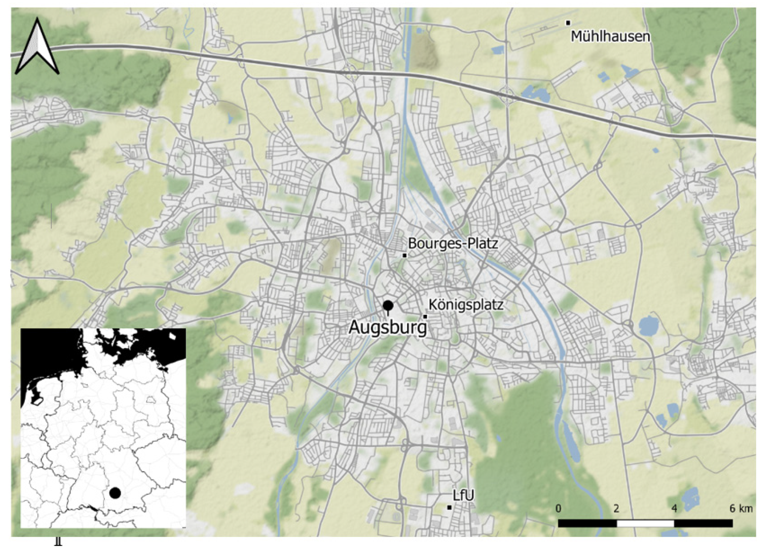
2.1. Air Quality and Meteorology Data

Air quality data were obtained from the online archive of the Bavarian Environmental Agency (Bayerisches Landesamt für Umwelt [15]). While, at first, all provided pollutants were considered, nitric oxides (NO & NO2), particulate matter (PM10 & PM2.5) and ozone (O3) were taken into the final analysis, after having passed tests for homogeneity and completeness [16,17]. Although the analysed datasets were all classified as ‘useful’, there were a few occasions in which a break was detected for NO and NO2 in the year 2010. This is in accordance with the implementation of the ‘Low Emission Zone’ in Augsburg, which led to slight but significant reductions in nitric oxide concentrations [18]. As we were interested in connections with ambient air pollution and the atmospheric circulation, we used background stations within the urban area of Augsburg in order to avoid influences from heavy traffic. Primarily, the suburban background station located at the Bavarian Environmental Agency (A-LfU) was used. Due to missing values, suburban NO und NO2 datasets were replaced by measurements at Augsburg-Bourges-Platz (urban background). While all data are provided on an hourly basis, ozone values were aggregated to the daily maximum, and nitric oxides, and particulate matter were aggregated to the daily mean.
Daily meteorological data originated from the Augsburg-Mühlhausen measuring station, operated by the German Weather Service (Deutscher Wetterdienst [19]). The selected variables were the daily minimum, mean and maximum temperatures; the mean humidity; the mean and maximum wind speeds; the rainfall amount and the mean pressure. The meteorological datasets were also ‘complete’ and classified as ‘useful’. All predictors and the measuring entities are listed in Table 1, and the study region is shown in Figure 1.

2.2. Cancer Mortality Data

The anonymised dataset of the Bavarian Cancer Registry (Augsburg Regional Center) [20], which comprises around 40,500 deaths of patients with an underlying cancer diagnosis in the period 2000 to 2017, serves as a medical basis. The data provide information on the date of death, zip code of residence, gender and age, as well as the type of cancer. The latter includes the specification of the International Classification of Diseases code (ICD-10). We included patients who had a diagnosis assigned to ICD-10-chapter II, block C00-D48 (Neoplasms) [21]. In our study, 15,601 patients residing in the Augsburg urban area (first three zip code numbers 861) were included. For the remaining patients residing outside Augsburg, exposure to the meteorological and air-hygienic conditions in Augsburg could not be assumed. The analysis was carried out for the period 2000–2017. As stated by Grundmann et al. [22], for Augsburg, there has been a recent decline in incidence for some cancer entities. Still, cancer remains a predominant factor in mortality, with 29% of all diseased individuals in 2017 having had a documented cancer diagnosis. We also found this trend in our analysis. In order to compare cancer mortality with the total mortality in the city of Augsburg, mortality data from the Bavarian State Office for Statistics [23] were also included.
Regarding the medical relevance and possible preventive measures when considering the mortality of cancer patients, days with a significantly increased number of deaths were of particular interest. The 95th percentile proved to be suitable for defining these cancer-related high mortality events. In this case, enough days were included in the analysis so that the effect of an outlier did not distort the statistical characteristics, while at the same time, the events remained within the range of extremes. Our data showed an annual cycle of daily death totals, with higher total sums in winter. To avoid the influence of seasonality on the selection of high-mortality events, the 31-day moving 95th percentile was computed for each calendar day and defined as the threshold. Specifically, the corresponding 95th percentile had to be exceeded to recognise a specific day as a high-mortality event. Thus, in summer, an event was defined as a daily sum of deaths of 6 or higher; in winter, this was 7 deaths or higher. Out of the 6575 days analysed between 2000 and 2017, 222 days exceeded the corresponding threshold and were considered cancer-related high-mortality events.

2.3. SLP Reanalysis Data

For the computation of the t-mode PCA, gridded daily mean sea level pressure data were obtained from the ERA5 reanalysis for the period 2000–2017, provided by the European Centre for Medium-Range Weather Forecasts (ECMWF, [24]). Computations were performed for a 1° × 1° grid in the 25° W–40° E and 25° N–70° N domain. Augsburg is located near the center of the domain at 48.3° N, 10.9° E.

2.4. Trends and Seasonality

To account for trends and seasonality, each meteorological and air-quality-related variable firstly underwent a detrending process. A variety of methods for detrending exist [25,26,27]. We followed an approach in accordance with Iler et al. [28] and applied a simple linear regression to each variable. The original data were then subtracted from the regression values; hence the residuals underwent further analysis as detrended values. In order to account for seasonality, for each calendar day, a 31-day moving average was computed and then subtracted from the corresponding detrended data. We, therefore, considered detrended, season-adjusted daily anomalies of atmospheric predictors in our study. Under this setup, negative (positive) values of predictors described a below-average (above-average) state regarding the corresponding moving average of the specific day. This approach has also been used in former studies [29,30,31].

2.5. Mann–Whitney U Test and Predictor Correlations

To find significant anomalies in meteorological and air quality data when comparing high with average mortality events, a Mann–Whitney U test [32,33] was carried out, as the predictor variables did not follow a normal distribution. Analyses were done for 3-month seasons. The mortality event days as well as up to 13 lead days were used. Lead days were not considered singularly, but comprised all days in a specific lead period, including the event day. We sought to find the unique influence of each variable on high-mortality days. In this regard, the necessity of a case-crossover design was evaluated by Spearman correlation coefficients between the various predictor variables (Figure 2).
Predictors of non-similar types (e.g., temperature-related, and ozone-related) with an absolute correlation coefficient higher than 0.7 (i.e., 50% shared variance) for three or more consecutive months were subject to a case-crossover analysis, while non-correlated predictors underwent U testing directly. Note that if more than one variable of a similar type required case-crossover analysis (e.g., TM and TX regarding ozone), only one variable of the specific type was regarded, according to the largest range of months with |r| > 0.7 and the absolute sum of explained variance. Case-crossover analysis was applied on a single-monthly basis if at least one month in a 3-month-moving window complied with the requirements for case-crossover. Afterwards, results were aggregated back to a three-monthly window.

2.6. Case-Crossover

Case-crossover analysis, as suggested by Pinheiro et al. [34], aims to uncover unique effects of predictors by controlling a specific variable by its high-correlated, confounding variables. By applying this procedure, the values of a specific variable on high-mortality days (=case) were tested against values on average mortality days (=control) by matching case days to corresponding control days with the highest similarity in the correlated variables. In our study, we developed a form of case-crossover analysis that was optimally adapted for our data in accordance with Pinheiro et al. with the following conditions: control days had to be dated within the same month, although we did not distinguish between different days of the week. This was due to the lack of control days when applying the case-crossover analysis to lead periods. In our case, a control value was determined by the least error sum of the correlated variables for the purpose of integrating lead periods. Hence, we integrated control periods instead of single control days. The deviation of all case and control values within a 14-day period was weighted and summed for every control period candidate. Weighting was applied using a half-normal distribution so that the error near a high-mortality event was given greater importance than deviations of more remote days. This procedure also allowed for the consideration of more than one control variable. All case periods and the corresponding control periods with the lowest overall weighted error sum for their preceding period subsequently underwent U testing. Variables requiring case-crossover procedures, the corresponding control variables and the months in which case-crossover was necessary are shown in Figure 2.

2.7. Principal Component Analysis (PCA)

For a deeper climatological interpretation of relevant months and lead periods before high-mortality events, the underlying atmospheric circulation, resp. weather types, was considered. This provided information about the general temperature and humidity conditions and the accumulation of airborne substances. In addition, the lateral transport of airborne substances can be explained by the resulting atmospheric flow during a specific weather situation.
While U testing was used to provide overall information on significant months and lead periods regarding high-mortality events on a single-predictor basis, we further characterised these specific time periods by applying PCA to the sea level pressure data from the ERA5 reanalysis dataset. Before the application of the PCA, we reduced the complexity of weather situations by combining contemporaneous predictors, i.e., they underwent processing in order to find the optimum months and lead period. Firstly, we defined a maximum time range by using the maximum outer extent of monthly windows and lead periods, in which every included predictor of interest showed significant U test results. Secondly, for every possible option within the maximum extent (m lead periods x n months) the quotient of the reduction in size compared with the maximum extent and the ratio of time steps in which not every predictor was significant was computed. The optimum time range was determined by the combination of m and n with the highest quotient value. For this optimum time range, a t-mode rotated PCA (VARIMAX) (e.g., Philipp [35], Huth [36]) was applied. Thus, as input, the sequence of days from the identified optimum lead time up to the mortality event day were entered into the PCA, as output weather type sequences typical for mortality events were generated.

3. Results

3.1. Cancer-Related High-Mortality Events

Deaths within cancer-related mortality events were found to be distributed unequally among age groups, with about 55% in patients aged 75 years or older (higher female rate than male), about 37% in the 55–74 age group (higher male rate), and just under 8% in the 25–54 age group (balanced rates). The most common underlying cancer was lung cancer (ICD C34, 12%). This was followed by breast cancer (ICD C50, 10%), colorectal cancer (ICD C18, 8.5%) and prostate cancer (ICD C61, 8%). With respect to the annual distribution of mortality events, a high level of similarity between summer (110 events) and winter (112 events) was found due to the choice of a moving percentile. In this context, it must be noted that the original total sum of deaths was higher in winter (780) than in summer (705). Additionally, looking at the monthly sum, months with an increased number of deaths in cancer-related mortality events were detected (January, April, July, October) next to months with a low total sum of deaths on event days (February, June, September, December).
Across all high-mortality events, there were minimal within-group differences in the characteristics of age groups, genders, and cancer types. Although it must be noted that, while most diagnosis groups showed higher total sums of deaths on event days in winter, a reverse effect was found to occur for patients with breast cancer, resulting in a higher total sum of daily deaths in summer. This surplus was greatest in July and August. Cancer-related mortality events did not occur in clusters and can, therefore, be understood as individual peaks. During winter, events were followed by other events on the following day only four times throughout the considered 18-year period. In summer, this only occurred three times. Spells longer than two days did not occur.

3.2. Relations to Weather and Air Quality

For various atmospheric parameters, significant anomalies were revealed in the U test in the run-up to cancer-related mortality events (Figure 3). Regarding air pollutants, NO2 and PM2.5 appear to be particularly relevant. In the case of meteorological variables, temperature anomalies, in particular, were prominent. Air pressure also showed significant manifestations in many cases, although these were primarily relevant in climatological interpretation. Significantly higher NO2 concentrations occurred in February through July, approximately 4 days to two weeks before mortality events. Elevated PM2.5 concentrations were significant for February through May between 10 and 13 days in advance of mortality events. In the case of temperature, various significant relationships emerged. Between October and March, higher than usual temperatures occurred throughout the two weeks prior to corresponding high-mortality events. Between February and May, cool minimum temperatures were often significantly prominent in the medium- to long-term lead-up. During summer and fall (June through October), a combination of significantly warmer maximum and cooler minimum temperatures was observed.
Temporally overlapping significant anomalies of multiple variables were combined in the form of composites. Increased concentrations of NO2 and PM2.5 occurred between February and April, together with lower than usual minimum temperatures, 12–13 days before a mortality event. This effect also occurred 4–5 days before an event when considering February through May, as well as a combined effect of NO2 and PM2.5 10–13 days before an event. In the medium-term lead period (6–9 days), elevated NO2 concentrations occurred between April and June in association with cooler mean and maximum temperatures. Significantly above-average mean and maximum temperatures occurred in summer and early fall (June through September) 3–8 days before an event, coinciding with below-average low temperatures during a more extended lead period (7–13 days). O3 also exhibited a coupled effect with maximum temperature 10–13 days before corresponding mortality events in fall. Subsequently, t-mode PCA was applied to the detected composites. The composites are recorded in Table 2.
First, a single high-mortality event within a specified time range was assigned to its matching principal component (PC) by the highest absolute correlation coefficient (loading) to the scores obtained from PCA. Within a selected PC, the atmospheric states in advance of each assigned event could be demonstrated and explained by the atmospheric circulation (scores) proposed by PCA. Means of relevant variables are given for corresponding lead days assigned to a similar PC. Means in the following text only represent cases in which an event had positive loading towards the illustrated atmospheric state, as cases with negative loadings were neglected due to low occurrence (1 in 52). It is important to note that different or contradictory results regarding U testing might occur when analysing event-based variables, as U test samples contain every event, while score-allocated samples represent a subset. The overall findings of the PCA outputs are addressed in the discussion section. In the following text, we demonstrate the capabilities of this approach by exemplifying it for a specific composite. We selected the fourth composite (Table 2), for which U testing suggested above average NO2 concentrations as well as below average mean and maximum temperatures in April through June.

3.3. PCA Results

PCA applied to composite number 4 suggests eleven PCs, with an overall explained variance of 82%. We take a closer look at the first, second, fourth and fifth PC. The third PC comprises a strong westerly flow over the target region resulting in low pollutant concentrations and was therefore left out in the detailed analysis. PCs one and two inherit the highest frequency and largest values of explained variance, PCs four and five are less frequent but inherit notable conditions of high interest. Composite number 4 shows significant impacts of predictors for the days 9 to 6 in advance of a high mortality event during April through June. The consecutive period of the ninth to sixth day before every high mortality event during April through June is treated as a unit and handed to PCA. Under this setup, the application of PCA makes it possible to investigate typical sequences of weather patterns that occur during the given consecutive days in advance of high mortality events. The resulting PCs each represent one of the typical sequences of weather patterns, that is followed by a high mortality event. In the case of composite number 4, the high mortality event occurs 6 days after the last day of the given sequences.

3.3.1. PC 1

PC 1 accounted for 13.9% of the explained variance and was assigned to 19% of the 52 events. Under the given atmospheric state, Augsburg was under the influence of a distinct high-pressure system over Scandinavia and Eastern Europe, intensifying throughout the considered sequence (Figure 4). The resulting conditions comprised a persistent easterly flow throughout the entire lead period, connected with clear conditions and the advection of warm and dry continental air masses. However, especially in spring (April, May), clear skies resulted in strong nocturnal cooling, causing low minimum temperatures. These thermal effects were shown by an increased daily maximum temperature by up to 1.9 K, near-average mean temperatures as well as mostly below-average minimum temperatures. Within a period of three days mean NO2 concentrations increased from below-average to about 7.5–8.5 µg/m3 above normal. This increase led to significantly higher concentrations compared with non-event-related days during the April to June period. Comparable increases toward significantly higher concentrations were also detected for PM10 and PM2.5. Causes for this could be increased emissions from heating, especially during cold nights, as well as air pollution accumulation in the lower atmosphere due to low-flow inversion-type conditions. Regarding high PM-concentrations, lateral transportation from Eastern Europe must also be considered.

3.3.2. PC 2

Nineteen percent of all events that occurred in April through June were assigned to this PC, accounting for an explained variance of 11.7%. Although there were similarities to PC 1 concerning the atmospheric circulation, PC 2 showed a pronounced high-pressure system shifted to the east and reaching further into Central Europe (Figure 5). Therefore, Augsburg was affected by weak easterly flows of dry-continental airmasses and clear skies. Again, the effect of nocturnal cooling was expressed by below-average minimum temperatures. The plotted weather sequence showed a continuing persistence of this weather type, leading to steadily increasing mean and maximum temperatures, reaching significantly higher than usual levels. Throughout the four-day period, concentrations of air pollutants were mostly above average, reaching significance for NO2 and PM10 six days before a high-mortality event.

3.3.3. PC 4

Three out of 52 events were assigned to the fourth PC, which accounted for 9.2% of the explained variance. In this case, a high-pressure system was dominant over the British Isles (Figure 6). Throughout the period, the high-pressure ridge reached out to the Mediterranean, thus also affecting Central Europe. At first, flows in Augsburg originated from the eastern direction. The change in the position of the high-pressure system as well as the persistent extension of the ridge caused the wind direction to shift north. Advection of polar airmasses resulted in below-average temperatures, as expected. Although PM concentrations were mostly lower as usual, a marked increase throughout the period was observed. NO-concentrations started at below-average values as well and experienced a mean relative increase of almost 13 µg/m3 within two days.

3.3.4. PC 5

PC 5 accounted for 7.3% of the explained variance and included six mortality events in cancer patients. Throughout the period, Augsburg was persistently under the influence of a low-pressure system, which slowly shifted its center from Central to Eastern Europe (Figure 7). During the period, the low-pressure system varied in intensity. Resulting flows in Augsburg, therefore, shifted from northwest to north and, eventually, northeast, transporting cool airmasses in combination with windy and rainy conditions under the influence of a low pressure. This resulted in below-average temperatures. In cases of mean and maximum temperatures, they were several K below usual, and this effect was highly significant when compared with non-event-related days in the same period. While mean anomalies were mostly significantly lower than usual for NO2 and PM10, PM2.5 experienced a slight increase towards the end of the period. In addition, it must be noted that NO2-concentrations, while remaining below average, increased similarly to the other inspected PCs, in this case by about 7 µg/m3 within two days.

3.4. Relationship of Cancer-Related Mortality Events to Non-Cancer-Related Mortality

For the comparison with the total mortality in Augsburg, the daily sum of cancer-related deaths was first subtracted from the total mortality rate. This concerned 29.6% of all deceased patients, as also been stated by Grundmann et al. [22]. After applying the Spearman correlation analysis, no statistical relationship was found between daily cancer-related deaths in Augsburg and the remaining daily mortality (rs ≈ −0.07, p ≈ 0). We then conducted an analysis of moderate extreme events for the remaining daily mortality by applying the procedure described in Section 2.5 and Section 2.6. According to our definition, a non-cancer-related extreme event was recorded if the daily sum exceeded 10–11 cases, depending on the respective day in summer, and 11–12 cases in winter. Temporal coincidence of the 95th percentile-based high mortality events in cancer patients and non-cancer-related mortality events showed no significant overlaps. However, U testing and case-crossover analysis, under the identical setup previously described, showed interesting results regarding similarities and differences to cancer-related events.
The U test significance and the indication of the overall mean difference between non-cancer related event days and non-event days, analogous to Figure 3, are provided in the Supplementary Materials Figure S1. Several variables with a high relevance for cancer also appeared to be significant for non-cancer-related extreme events, including NO2, PM2.5 and the minimum temperature. For the former two, this included significantly above-average concentrations in late summer through winter. Minimum temperatures deviated significantly to negative values in late winter and appeared above-average in summer and fall. However, although a similarity in the overall importance of these variables for cancer- and non-cancer-related mortality events was detected, it became clear that there were notable variations in the direction of the effect (positive or negative) as well as with respect to the relevant months and lead times of these predictors. Other predictors with no significant effects on cancer-related mortality appeared to be significant for non-cancer-related mortality. This, for example, included significantly above-average O3 concentrations in summer and fall as well as significantly below-average relative humidity, coupled with overall below-average temperatures in winter through early spring.

4. Discussion

The discussion of our results can be divided into two sections. Firstly, the relationship between atmospheric states and the occurrence of cancer-related moderate high mortality events is covered. Secondly, we detail the information gained through the application of climatological methods to medical data.
While the assessment of long-term effects remains a major part of epidemiological research, we aimed to present the short-term effects of meteorology and air quality on cancer-related mortality in Augsburg, Southern Germany during the 2000–2017 period. We focused on moderate extreme events regarding mortality by defining the 31-day-moving 95th percentile as the threshold for cancer-related mortality events. The medical evidence states that carcinogenesis is mostly affected by long-term factors, i.e., persistent exposure to pollutants, such as particulate matter [14,37,38,39]. Short-term effects place an additional burden on cancer patients. An organism that is additionally burdened, for example, by increased pollutant concentrations or significantly low or high temperatures, has greater susceptibility to the onset of additional diseases, mainly of a respiratory nature [40,41], which, in turn, promote premature death. Our study suggests that above-average concentrations of NO2 and PM2.5 as well as temperature-related effects contribute the most regarding these burdens for individuals in Augsburg, predominantly occurring one to two weeks before death events.
NO2 showed significantly above-average anomalies, beginning in February and lasting until mid-summer. These anomalies mostly occurred 4 to 13 days before a mortality event. Higher than usual PM2.5 concentrations occurred from February to May, preceding high-mortality events by 10 to 13 days. Above-average concentrations during this period often occurred in combination with lower than usual temperatures. From summer through autumn, significantly above-average maximum and mean temperatures occurred in combination with below-average minimum temperatures in advance of mortality events. Our analysis indicates that lag effects for warmer temperatures are shorter (3–8 days) when compared with low temperatures (7–13 days). Another season with significantly above-average temperatures was shown to be winter, from November through February.
The finding that there is an overall higher risk of death under extreme weather conditions and bad air quality is in accordance with other studies [42,43,44,45,46]. A strong link to respiratory mortality can be assumed. Many authors have indicated that there is a strong link between respiratory mortality and short-term exposure to increased levels of ambient PM2.5 and SO2 [47,48,49]. While SO2 was excluded from our analysis, our study confirms the major role of PM2.5. Recent studies have also indicated the adverse respiratory health effects of increased NO2 levels [50,51]. A study distinguishing between respiratory-related and cancer-related deaths found a distinct increase in mortality risk among lung-cancer patients when exposed to high levels of ambient NO2 [52]. A recently published meta-analysis showed strong evidence of adverse effects of high PM2.5 and NO2 concentrations, among other pollutants, and a resulting increase in cancer-related mortality [4]. The authors also pointed out the limitations of these studies, especially the focus on non-lung-related cancer types, and the need for further research. Although our data suggest a strong link between PM10 and PM2.5, the isolated analysis of both variables in our case showed notable, significant anomalies only for the latter. The PCA analysis, in turn, revealed significantly high levels of PM10, in connection with favorable synoptic conditions.
In the context of temperature, our findings were mostly in accordance with previous studies. While specifically cancer-related analyses regarding temperature extremes are scarce, an increase in overall mortality with significantly low or high temperatures has been observed [53]. While elderly patients form the largest group regarding cancer-mortality, it must be noted that, in this context, elderly patients are generally more likely to be affected by significant temperature anomalies.
An increase in air pollution concentrations can stem from three major causes: in situ formation, accumulation and lateral transport. Favourable conditions for the accumulation of air pollutants include low wind speeds and no washout by precipitation [54,55]. These conditions are best-matched with anticyclonic and low-flow patterns in general and become particularly relevant in winter when temperatures are low and emissions from traffic and heating are high. Lateral transport of airborne substances, in general, can lead to an increase in concentrations, in particular when originating from specific locations such as traffic- or industry-intense and highly populated urban areas. For our study site, specific conditions apply. As a study conducted in Germany [56] pointed out, lateral transport from western European locations plays only a minor role, whereas flows originating from Eastern Europe become dominant in this context. In combination with high pollutant concentrations over Southern and Eastern Europe [57,58], lateral transport under weak easterly to southerly flows and dry conditions must be considered when analysing bad air quality at our study site. For composites 1–4, above-average NO2 and particulate matter concentrations as well as below-average temperatures were detected. The PCA suggested that these conditions are caused by (a) anticyclonic conditions with southerly to easterly flows and (b) low-flow conditions. Warm temperature anomalies in summer and early fall (composites 5–7) were accompanied by low levels of cloud coverage, allowing for intense radiation, as well as subtropical flows with southern origins. Nocturnal cooling increased in the further course of late summer to fall, resulting in below-average minimum temperatures. Significantly above-average temperatures from November through February can be explained by a dominant impact of westerly flows, bringing Augsburg under the influence of warmer maritime air masses. This is contradictory to the other results, as positive temperature anomalies in winter in our domain refer to overall mild conditions, bearing no adverse health effects. However, PCs 3 and 4 of this period, which had an explained variance of 22%, described a strong anticyclonic influence, resulting in easterly flows, leading to deviations of up to 3.3 K below average for minimum and 4.5 K below average for maximum temperatures. This, in turn, is in accordance with the results of previous studies concerning the health effects of low temperature extremes.
Although a significant contribution of atmospheric predictors can be established, it must, nevertheless, be noted that other, non-atmospheric factors contribute to cancer mortality as well [59,60,61]. In our case, we focused solely on the effects of atmospheric predictors on extreme cancer-related mortality events. To account for non-atmospheric factors, more detailed information about the patients would be necessary, e.g., cause of death, lifestyle parameters, place of residence and pre-existing conditions. Further advancements could also be achieved by incorporating more cases in a cross-regional analysis.
Predominant predictors regarding cancer-related mortality can also be of high relevance for non-cancer-related mortality. This is in accordance with the former studies discussed above and comprises NO2, PM2.5 and deviations in temperature. However, there appear to be significant differences in the seasonal and temporal (lead time) characteristics of these predictors as well as in the overall direction of the effects. The latter is, for example, expressed by below-average temperatures for non-cancer-related mortality events from January through March, while the opposite is the case for cancer-related events. Adverse effects of low temperatures on overall mortality were, for example, pointed out by Gasparrini et al. [43]. Additionally, ozone appears to be of high importance for non-cancer mortality, which is supported by the findings of Hertig et al. [62,63]. Still, these findings must be interpreted cautiously, as patient information in the overall mortality dataset is limited. Due to this, we could not distinguish influential pre-existing conditions and the cause of death. Further analysis could be useful for providing a deeper understanding of these links in future studies.
Regarding methods, our study shows the potential of statistical hypothesis testing as an alternative to the use of statistical models. This applies, in particular, when modeling is aggravated, e.g., due to a low number of cases. U testing can provide a broad overview of links between medical data and atmospheric predictors. Its strengths lie in the analysis of seasonality and lag-periods. While overall responses become clear, the specific meteorological conditions in the period before such mortality events remain unknown. We, therefore, applied PCA to the results of predictor-based U testing and highlighted the range of meteorological conditions linked with the corresponding period. This approach clearly demonstrated that specific meteorological and air pollution anomalies need not stem from the same weather types. An in-depth analysis of weather types, in particular weather sequences, allowed for a robust interpretation of the relevant anomalies.

5. Conclusions

In our study, we found significant deviations in meteorological and air quality variables in the run-up to cancer-related mortality events. We found the main drivers to be elevated NO2 and PM2.5 concentrations in the late winter to early summer period, together with below-average minimum temperatures. In summer and fall, cancer-related mortality events were linked with significantly higher mean and maximum air temperatures. More than half of the decedents considered were 75 years or older, and more than 90% were older than 54. The total number of decedents was higher in winter than in summer. An exception was the group of breast cancer patients, for whom increased mortality occurred in summer. The combination of pathophysiological and climatological views on the present results suggests that the influences of air quality and weather do not have direct short-term effects on carcinogenesis, but rather, represent an additional burden on cancer patients. We also inspected the impacts of the meteorological and air quality variables on overall mortality. Although predominant predictors for cancer-related mortality are also of high importance for non-cancer-related mortality, noticeable differences regarding the characteristics of the relationships were shown. The results show the potential for further investigations of the relationship between cancer mortality and atmospheric conditions. A detailed knowledge base about the atmospheric conditions in the run-up to cancer-related mortality events could help to identify and predict adverse atmospheric conditions in advance of their occurrence and, thus, could be used to enhance the preparedness and response within health care.

Supplementary Materials

The following is available online at https://www.mdpi.com/article/10.3390/ijerph182211737/s1, Figure S1: U test results of meteorological and air quality predictors regarding noncancer-related mortality events.

Author Contributions

Conceptualization, I.K.-O., E.H. and M.T.; methodology, P.O., I.K.-O., S.K., G.S., M.T. and E.H.; formal analysis, P.O., I.K.-O., S.K., E.H.; investigation, P.O., I.K.-O., S.K., M.T. and E.H.; data curation, P.O., G.S. and E.H.; writing—original draft preparation, P.O.; writing—review and editing, P.O., I.K.-O., S.K., M.T. and E.H.; visualization, P.O. and I.K.-O.; supervision, E.H.; funding acquisition, I.K.-O., M.T. and E.H. All authors have read and agreed to the published version of the manuscript.

Funding

This research received funding from the Faculty of Medicine, University of Augsburg. This work was also supported by the Deutsche Forschungsgemeinschaft (DFG, German Research Foundation) under project number 408057478.

Institutional Review Board Statement

The study was conducted according to the guidelines of the Declaration of Helsinki and approved by the Institutional Review Board of Augsburg University Medical Center (protocol code 2020-25, date of approval 5 July 2020).

Informed Consent Statement

Patient consent was waived due to the use of anonymised registry data of deceased persons only.

Data Availability Statement

Publicly available datasets were analyzed in this study. This includes (a) station-based meteorological data, (b) air quality data and (c) reanalysis data. This data can be found here: (a) https://opendata.dwd.de/climate_environment/CDC/observations_germany/climate/daily/kl/historical/tageswerte_KL_00232_19470101_20201231_hist.zip; (b) https://www.lfu.bayern.de/luft/immissionsmessungen/messwertarchiv/index.htm; (c) https://cds.climate.copernicus.eu/cdsapp#!/dataset/reanalysis-era5-single-levels?tab=overview. Restrictions apply to the availability of (a) cancer-related mortality data and (b) overall mortality. (a) was obtained from the Bavarian Cancer Registry and is available at https://www.lgl.bayern.de/gesundheit/krebsregister/auswertung_forschung/index.htm with the permission of the Bavarian Cancer Registry; (b) was obtained from the Bavarian State Office for Statistics and is available at https://www.statistik.bayern.de/statistik/gebiet_bevoelkerung/bevoelkerungsbewegung/index.html#link_2 with permission of the Bavarian State Office for Statistics (all accessed on 10 October 2021).

Conflicts of Interest

The authors declare no conflict of interest. The funders had no role in the design of the study; in the collection, analyses, or interpretation of data; in the writing of the manuscript, or in the decision to publish the results.

References

  1. Masson-Delmotte, V.P.; Zhai, A.; Pirani, S.L.; Connors, C.; Péan, S.; Berger, N.; Caud, Y.; Chen, L. (Eds.) International panel on climate change; summary for policymakers. In Climate Change 2021: The Physical Science Basis. Contribution of Working Group I to the Sixth Assessment Report of the Intergovernmental Panel on Climate Change; Cambridge University Press: Cambridge, UK, 2021. [Google Scholar]
  2. Sung, H.; Ferlay, J.; Siegel, R.L.; Laversanne, M.; Soerjomataram, I.; Jemal, A.; Bray, F. Global cancer statistics 2020: GLOBOCAN estimates of incidence and mortality worldwide for 36 cancers in 185 countries. CA Cancer J. Clin. 2021, 71, 209–249. [Google Scholar] [CrossRef]
  3. Cancer. Available online: https://www.who.int/news-room/fact-sheets/detail/cancer (accessed on 18 August 2021).
  4. Turner, M.C.; Andersen, Z.J.; Baccarelli, A.; Diver, W.R.; Gapstur, S.M.; Pope, C.A.; Prada, D.; Samet, J.; Thurston, G.; Cohen, A. Outdoor air pollution and cancer: An overview of the current evidence and public health recommendations. CA Cancer J. Clin. 2020, 70, 460–479. [Google Scholar] [CrossRef]
  5. Bray, F.; Ferlay, J.; Soerjomataram, I.; Siegel, R.L.; Torre, L.A.; Jemal, A. Global cancer statistics 2018: GLOBOCAN estimates of incidence and mortality worldwide for 36 cancers in 185 countries. CA Cancer J. Clin. 2018, 68, 394–424. [Google Scholar] [CrossRef] [Green Version]
  6. Khorrami, Z.; Pourkhosravani, M.; Rezapour, M.; Etemad, K.; Taghavi-Shahri, S.M.; Künzli, N.; Amini, H.; Khanjani, N. Multiple air pollutant exposure and lung cancer in Tehran, Iran. Sci. Rep. 2021, 11, 9239. [Google Scholar] [CrossRef]
  7. Hamra, G.B.; Guha, N.; Cohen, A.; Laden, F.; Raaschou-Nielsen, O.; Samet, J.M.; Vineis, P.; Forastiere, F.; Saldiva, P.; Yorifuji, T.; et al. Outdoor particulate matter exposure and lung cancer: A systematic review and meta-analysis. Environ. Health Perspect. 2014, 122, 906–911. [Google Scholar] [CrossRef] [Green Version]
  8. Turner, M.C.; Krewski, D.; Diver, W.R.; Pope, C.A.; Burnett, R.T.; Jerrett, M.; Marshall, J.D.; Gapstur, S.M. Ambient air pollution and cancer mortality in the cancer prevention study II. Environ. Health Perspect. 2017, 125, 087013. [Google Scholar] [CrossRef] [Green Version]
  9. Turner, M.C.; Gracia-Lavedan, E.; Cirac, M.; Castaño-Vinyals, G.; Malats, N.; Tardon, A.; Garcia-Closas, R.; Serra, C.; Carrato, A.; Jones, R.R.; et al. Ambient air pollution and incident bladder cancer risk: Updated analysis of the Spanish Bladder Cancer Study. Int. J. Cancer 2019, 145, 894–900. [Google Scholar] [CrossRef]
  10. Tagliabue, G.; Borgini, A.; Tittarelli, A.; van Donkelaar, A.; Martin, R.V.; Bertoldi, M.; Fabiano, S.; Maghini, A.; Codazzi, T.; Scaburri, A.; et al. Atmospheric fine particulate matter and breast cancer mortality: A population-based cohort study. BMJ Open 2016, 6, e012580. [Google Scholar] [CrossRef] [Green Version]
  11. White, A.J.; Keller, J.P.; Zhao, S.; Carroll, R.; Kaufman, J.D.; Sandler, D.P. Air pollution, clustering of particulate matter components, and breast cancer in the sister study: A U.S.-wide cohort. Environ. Health Perspect. 2019, 127, 107002. [Google Scholar] [CrossRef]
  12. Hwang, J.; Bae, H.; Choi, S.; Yi, H.; Ko, B.; Kim, N. Impact of air pollution on breast cancer incidence and mortality: A nationwide analysis in South Korea. Sci. Rep. 2020, 10, 5392. [Google Scholar] [CrossRef]
  13. Kazemiparkouhi, F.; Eum, K.-D.; Wang, B.; Manjourides, J.; Suh, H.H. Long-term ozone exposures and cause-specific mortality in a US Medicare cohort. J. Expo. Sci. Environ. Epidemiol. 2019, 30, 650–658. [Google Scholar] [CrossRef] [Green Version]
  14. Lequy, E.; Siemiatycki, J.; de Hoogh, K.; Vienneau, D.; Dupuy, J.-F.; Garès, V.; Hertel, O.; Christensen, J.H.; Zhivin, S.; Goldberg, M.; et al. Contribution of long-term exposure to outdoor black carbon to the carcinogenicity of air pollution: Evidence regarding risk of cancer in the gazel cohort. Environ. Health Perspect. 2021, 129, 37005. [Google Scholar] [CrossRef]
  15. Bayerisches Landesamt für Umwelt. Messwertarchiv [Archive of Measurement Values]. Available online: https://www.lfu.bayern.de/luft/immissionsmessungen/messwertarchiv/index.htm (accessed on 10 October 2020).
  16. Moberg, A.; Jones, P.D.; Lister, D.; Walther, A.; Brunet, M.; Jacobeit, J.; Alexander, L.; Della-Marta, P.M.; Luterbacher, J.; Yiou, P.; et al. Indices for daily temperature and precipitation extremes in Europe analyzed for the period 1901–2000. J. Geophys. Res. Atmos. 2006, 111. [Google Scholar] [CrossRef] [Green Version]
  17. Wijngaard, J.B.; Tank, A.K.; Können, G.P. Homogeneity of 20th century European daily temperature and precipitation series. Int. J. Clim. 2003, 23, 679–692. [Google Scholar] [CrossRef]
  18. Morfeld, P.; Groneberg, D.A.; Spallek, M.F. Effectiveness of low emission zones: Large scale analysis of changes in environmental NO2, NO and NOX concentrations in 17 German cities. PLoS ONE 2014, 9, e102999. [Google Scholar] [CrossRef] [Green Version]
  19. Climate Data Center. Available online: https://opendata.dwd.de/climate_environment/ (accessed on 19 May 2021).
  20. Bayerisches Krebsregister. Regionalzentrum Augsburg. Available online: https://www.lgl.bayern.de/gesundheit/krebsregister/index.htm (accessed on 17 August 2021).
  21. International Statistical Classification of Diseases and Related Health Problems 10th Revision. Available online: https://icd.who.int/browse10/2010/en (accessed on 17 September 2021).
  22. Grundmann, N.; Meisinger, C.; Trepel, M.; Müller-Nordhorn, J.; Schenkirsch, G.; Linseisen, J. Trends in cancer incidence and survival in the Augsburg study region—Results from the Augsburg cancer registry. BMJ Open 2020, 10, e036176. [Google Scholar] [CrossRef]
  23. Natürliche Bevölkerungsbewegung—Sterbefälle. Available online: https://www.statistik.bayern.de/statistik/gebiet_bevoelkerung/bevoelkerungsbewegung/index.html#link_2 (accessed on 18 August 2021).
  24. Hersbach, H.; Bell, B.; Berrisford, P.; Hirahara, S.; Horanyi, A.; Muñoz-Sabater, J.; Nicolas, J.; Peubey, C.; Radu, R.; Schepers, D.; et al. The ERA5 global reanalysis. Q. J. R. Meteorol. Soc. 2020, 146, 1999–2049. [Google Scholar] [CrossRef]
  25. Botlaguduru, V.S.V.; Kommalapati, R.R. Meteorological detrending of long-term (2003–2017) ozone and precursor concentrations at three sites in the Houston Ship Channel Region. J. Air Waste Manag. Assoc. 2019, 70, 93–107. [Google Scholar] [CrossRef]
  26. Sohail, H.; Kollanus, V.; Tiittanen, P.; Schneider, A.; Lanki, T. Heat, heatwaves and cardiorespiratory hospital admissions in Helsinki, Finland. Int. J. Environ. Res. Public Health 2020, 17, 7892. [Google Scholar] [CrossRef]
  27. Wu, Z.; Huang, N.E.; Long, S.R.; Peng, C.-K. On the trend, detrending, and variability of nonlinear and nonstationary time series. Proc. Natl. Acad. Sci. USA 2007, 104, 14889–14894. [Google Scholar] [CrossRef] [Green Version]
  28. Iler, A.M.; Inouye, D.W.; Schmidt, N.M.; Høye, T.T. Detrending phenological time series improves climate–phenology analyses and reveals evidence of plasticity. Ecology 2017, 98, 647–655. [Google Scholar] [CrossRef] [Green Version]
  29. Tai, A.P.K.; Mickley, L.J.; Jacob, D.J. Correlations between fine particulate matter (PM2.5) and meteorological variables in the United States: Implications for the sensitivity of PM2.5 to climate change. Atmos. Environ. 2010, 44, 3976–3984. [Google Scholar] [CrossRef]
  30. Gosling, S.N.; McGregor, G.R.; Páldy, A. Climate change and heat-related mortality in six cities Part 1: Model construction and validation. Int. J. Biometeorol. 2007, 51, 525–540. [Google Scholar] [CrossRef]
  31. Rooney, C.; McMichael, A.J.; Kovats, R.S.; Coleman, M.P. Excess mortality in England and Wales, and in Greater London, during the 1995 heatwave. J. Epidemiol. Community Health 1998, 52, 482–486. [Google Scholar] [CrossRef] [Green Version]
  32. Mann, H.B.; Whitney, D.R. On a test of whether one of two random variables is stochastically larger than the other. Ann. Math. Stat. 1947, 18, 50–60. [Google Scholar] [CrossRef]
  33. Wilcoxon, F. Individual comparisons by ranking methods. Biom. Bull. 1945, 1, 80–83. [Google Scholar] [CrossRef]
  34. Pinheiro, S.L.L.A.; Saldiva, P.H.N.; Schwartz, J.; Zanobetti, A. Isolated and synergistic effects of PM10 and average temperature on cardiovascular and respiratory mortality. Rev. Saúde Pública 2014, 48, 881–888. [Google Scholar] [CrossRef] [Green Version]
  35. Philipp, A. Comparison of principal component and cluster analysis for classifying circulation pattern sequences for the European domain. Theor. Appl. Clim. 2008, 96, 31–41. [Google Scholar] [CrossRef]
  36. Huth, R. Properties of the circulation classification scheme based on the rotated principal component analysis. Meteorol. Atmos. Phys. 1996, 59, 217–233. [Google Scholar] [CrossRef]
  37. Hvidtfeldt, U.A.; Severi, G.; Andersen, Z.J.; Atkinson, R.; Bauwelinck, M.; Bellander, T.; Boutron-Ruault, M.-C.; Brandt, J.; Brunekreef, B.; Cesaroni, G.; et al. Long-term low-level ambient air pollution exposure and risk of lung cancer—A pooled analysis of 7 European cohorts. Environ. Int. 2021, 146, 106249. [Google Scholar] [CrossRef]
  38. Santovito, A.; Gendusa, C.; Cervella, P.; Traversi, D. In vitro genomic damage induced by urban fine particulate matter on human lymphocytes. Sci. Rep. 2020, 10, 8853. [Google Scholar] [CrossRef]
  39. Loomis, D.; Grosse, Y.; Lauby-Secretan, B.; El Ghissassi, F.; Bouvard, V.; Benbrahim-Tallaa, L.; Guha, N.; Baan, R.; Mattock, H.; Straif, K. The carcinogenicity of outdoor air pollution. Lancet Oncol. 2013, 14, 1262–1263. [Google Scholar] [CrossRef]
  40. Abdel-Rahman, O. Influenza and pneumonia-attributed deaths among cancer patients in the United States; a population-based study. Expert Rev. Respir. Med. 2021, 15, 393–401. [Google Scholar] [CrossRef]
  41. Elfaituri, M.K.; Morsy, S.; Tawfik, G.M.; Abdelaal, A.; El-Qushayri, A.E.; Faraj, H.A.; Hieu, T.H.; Huy, N.T. Incidence of infection-related mortality in cancer patients: Trend and survival analysis. J. Clin. Oncol. 2019, 37, e23095. [Google Scholar] [CrossRef]
  42. Vicedo-Cabrera, A.M.; Scovronick, N.; Sera, F.; Royé, D.; Schneider, R.; Tobias, A.; Astrom, C.; Guo, Y.; Honda, Y.; Hondula, D.M.; et al. The burden of heat-related mortality attributable to recent human-induced climate change. Nat. Clim. Chang. 2021, 11, 492–500. [Google Scholar] [CrossRef]
  43. Gasparrini, A.; Guo, Y.; Hashizume, M.; Lavigne, E.; Zanobetti, A.; Schwartz, J.; Tobías, A.; Tong, S.; Rocklöv, J.; Forsberg, B.; et al. Mortality risk attributable to high and low ambient temperature: A multicountry observational study. Lancet 2015, 386, 369–375. [Google Scholar] [CrossRef]
  44. Kloog, I.; Ridgway, B.; Koutrakis, P.; Coull, B.A.; Schwartz, J.D. Long- and short-term exposure to PM2.5 and mortality: Using novel exposure models. Epidemiology 2013, 24, 555–561. [Google Scholar] [CrossRef]
  45. Goldberg, M.S.; Gasparrini, A.; Armstrong, B.; Valois, M.-F. The short-term influence of temperature on daily mortality in the temperate climate of Montreal, Canada. Environ. Res. 2011, 111, 853–860. [Google Scholar] [CrossRef]
  46. Touloumi, G.; Pocock, S.J.; Katsouyanni, K.; Trichopoulos, D. Short-term effects of air pollution on daily mortality in athens: A time-series analysis. Int. J. Epidemiol. 1994, 23, 957–967. [Google Scholar] [CrossRef]
  47. Slama, A.; Śliwczyński, A.; Woźnica-Pyzikiewicz, J.; Zdrolik, M.; Wiśnicki, B.; Kubajek, J.; Turżańska-Wieczorek, O.; Studnicki, M.; Wierzba, W.; Franek, E. The short-term effects of air pollution on respiratory disease hospitalizations in 5 cities in Poland: Comparison of time-series and case-crossover analyses. Environ. Sci. Pollut. Res. 2020, 27, 24582–24590. [Google Scholar] [CrossRef]
  48. Mokoena, K.; Ethan, C.J.; Yu, Y.; Shale, K.; Liu, F. Ambient air pollution and respiratory mortality in Xi’an, China: A time-series analysis. Respir. Res. 2019, 20, 139. [Google Scholar] [CrossRef]
  49. Zhu, F.; Ding, R.; Lei, R.; Cheng, H.; Liu, J.; Shen, C.; Zhang, C.; Xu, Y.; Xiao, C.; Li, X.; et al. The short-term effects of air pollution on respiratory diseases and lung cancer mortality in Hefei: A time-series analysis. Respir. Med. 2019, 146, 57–65. [Google Scholar] [CrossRef]
  50. Meng, X.; Liu, C.; Chen, R.; Sera, F.; Vicedo-Cabrera, A.M.; Milojevic, A.; Guo, Y.; Tong, S.; de Sousa Zanotti Stagliorio Coelho, M.; Saldiva, P.H.N.; et al. Short term associations of ambient nitrogen dioxide with daily total, cardiovascular, and respiratory mortality: Multilocation analysis in 398 cities. BMJ 2021, 372, n534. [Google Scholar] [CrossRef]
  51. Ren, M.; Li, N.; Wang, Z.; Liu, Y.; Chen, X.; Chu, Y.; Li, X.; Zhu, Z.; Tian, L.; Xiang, H. The short-term effects of air pollutants on respiratory disease mortality in Wuhan, China: Comparison of time-series and case-crossover analyses. Sci. Rep. 2017, 7, 40482. [Google Scholar] [CrossRef]
  52. Xue, X.; Chen, J.; Sun, B.; Zhou, B.; Li, X. Temporal trends in respiratory mortality and short-term effects of air pollutants in Shenyang, China. Environ. Sci. Pollut. Res. 2018, 25, 11468–11479. [Google Scholar] [CrossRef] [Green Version]
  53. Breitner, S.; Wolf, K.; Devlin, R.B.; Diaz-Sanchez, D.; Peters, A.; Schneider, A. Short-term effects of air temperature on mortality and effect modification by air pollution in three cities of Bavaria, Germany: A time-series analysis. Sci. Total Environ. 2014, 485–486, 49–61. [Google Scholar] [CrossRef]
  54. Xu, Y.; Xue, W.; Lei, Y.; Zhao, Y.; Cheng, S.; Ren, Z.; Huang, Q. Impact of meteorological conditions on PM2.5 pollution in China during winter. Atmosphere 2018, 9, 429. [Google Scholar] [CrossRef] [Green Version]
  55. Jiang, N.; Hay, J.E.; Fisher, G.W. Effects of meteorological conditions on concentrations of nitrogen oxides in Auckland. Weather Clim. 2005, 24, 15–34. [Google Scholar] [CrossRef]
  56. Heintzenberg, J.; Birmili, W.; Hellack, B.; Spindler, G.; Tuch, T.; Wiedensohler, A. Aerosol pollution maps and trends over Germany with hourly data at four rural background stations from 2009 to 2018. Atmos. Chem. Phys. Discuss. 2020, 20, 10967–10984. [Google Scholar] [CrossRef]
  57. EEA. Air Quality in Europe—2020 Report; EEA Report, No. 09/2020; Publications Office of the European Union: Luxembourg, 2020. [Google Scholar]
  58. Eeftens, M.; Tsai, M.-Y.; Ampe, C.; Anwander, B.; Beelen, R.; Bellander, T.; Cesaroni, G.; Cirach, M.; Cyrys, J.; De Hoogh, K.; et al. Spatial variation of PM2.5, PM10, PM2.5 absorbance and PMcoarse concentrations between and within 20 European study areas and the relationship with NO2—Results of the ESCAPE project. Atmos. Environ. 2012, 62, 303–317. [Google Scholar] [CrossRef] [Green Version]
  59. Zhang, Y.-B.; Pan, X.-F.; Chen, J.; Cao, A.; Zhang, Y.-G.; Xia, L.; Wang, J.; Li, H.; Liu, G.; Pan, A. Combined lifestyle factors, incident cancer, and cancer mortality: A systematic review and meta-analysis of prospective cohort studies. Br. J. Cancer 2020, 122, 1085–1093. [Google Scholar] [CrossRef]
  60. Karavasiloglou, N.; Pestoni, G.; Wanner, M.; Faeh, D.; Rohrmann, S. Healthy lifestyle is inversely associated with mortality in cancer survivors: Results from the third national health and nutrition examination survey (NHANES III). PLoS ONE 2019, 14, e0218048. [Google Scholar] [CrossRef] [Green Version]
  61. Chen, G.; Wan, X.; Yang, G.; Zou, X. Traffic-related air pollution and lung cancer: A meta-analysis. Thorac. Cancer 2015, 6, 307–318. [Google Scholar] [CrossRef]
  62. Hertig, E.; Russo, A.; Trigo, R.M. Heat and ozone pollution waves in central and South Europe—Characteristics, weather types, and association with mortality. Atmosphere 2020, 11, 1271. [Google Scholar] [CrossRef]
  63. Hertig, E. Health-relevant ground-level ozone and temperature events under future climate change using the example of Bavaria, Southern Germany. Air Qual. Atmos. Health 2020, 13, 435–446. [Google Scholar] [CrossRef] [Green Version]
Figure 1. Location of meteorological and air quality measuring sites in Augsburg, Germany.
Ijerph 18 11737 g001
Figure 2. Monthly predictor correlation coefficients for all predictors with respect to the case-crossover analysis. Only coefficients >0.7 and <−0.7 (=shared variance approx. 50%) were plotted. Variables for which case-control was necessary are marked with *.
Ijerph 18 11737 g002
Figure 3. U test results for meteorological and air quality predictors regarding cancer-related mortality events. Monthly windows and up to 13 days prior to each event were considered. Variable abbreviations are listed in Table 1. Numbers next to monthly windows indicate the sum of mortality events within given months. Coloring refers to the mean difference of event-related days minus non-event-related days. Red indicates a significant positive deviation for high-mortality events, while blue indicates a significant negative deviation. P-values of significance are provided for three levels (0.01, 0.05, 0.1).
Ijerph 18 11737 g003
Figure 4. Weather sequence of PC 1 for lag days 9 to 6 before a high mortality event in April through June. Contours are scores of PC 1 and refer to the sea level pressure on a given day, with red indicating high pressure and blue indicating low pressure. Also given are mean predictor anomalies of all corresponding days of the same lag for air temperature and the chosen air pollutants (for abbreviations, see Table 1). Positive values indicate an above-average state, and negative values indicate a below-average state. If the values of a specific lag day deviate significantly from all non-high-mortality-related days within April through June, the level of significance is provided (***: 0.01; **: 0.05; *: 0.1; determined by U test) as well as the mean difference of all days of the same lag minus the mean of all non-high-mortality-related days, indicated by + or −. + indicates a higher anomaly mean on the corresponding lag days than on non-high-mortality-related days.
Ijerph 18 11737 g004
Figure 5. Same as Figure 4, but for PC 2. The level of significance is provided (**: 0.05; *: 0.1). The mean difference of all days of the same lag minus the mean of all non-high-mortality-related days, indicated by + or −. + indicates a higher anomaly mean on the corresponding lag days than on non-high-mortality-related days. − indicates a lower anomaly mean on the corresponding lag days than on non-high-mortality-related days.
Ijerph 18 11737 g005
Figure 6. Same as Figure 4, but for PC 4. The level of significance is provided (**: 0.05; *: 0.1). The mean difference of all days of the same lag minus the mean of all non-high-mortality-related days, indicated by + or −. + indicates a higher anomaly mean on the corresponding lag days than on non-high-mortality-related days. − indicates a lower anomaly mean on the corresponding lag days than on non-high-mortality-related days.
Ijerph 18 11737 g006
Figure 7. Same as Figure 4, but for PC 5. The level of significance is provided (***: 0.01; **: 0.05). The mean difference of all days of the same lag minus the mean of all non-high-mortality-related days, indicated by + or −. + indicates a higher anomaly mean on the corresponding lag days than on non-high-mortality-related days. − indicates a lower anomaly mean on the corresponding lag days than on non-high-mortality-related days.
Ijerph 18 11737 g007
Table 1. Included atmospheric predictors, corresponding measuring sites and measuring entities.
Abb.VariableUnitMeasuring SiteMeasuring Entity
NOnitric oxideµg/m3A-Bourges-PlatzLfU Bayern
NO2nitrogen dioxideµg/m3A-Bourges-PlatzLfU Bayern
PM10particulate matterµg/m3A-LfULfU Bayern
PM2.5particulate matterµg/m3A-LfULfU Bayern
O3ozoneµg/m3A-LfULfU Bayern
TNminimum temperature°CA-MühlhausenDWD
TMmean temperature°CA-MühlhausenDWD
TXmaximum temperature°CA-MühlhausenDWD
RHrelative humidity%A-MühlhausenDWD
FMmean wind speedms−1A-MühlhausenDWD
FXmaximum wind speedms−1A-MühlhausenDWD
Rrainfall amountmmA-MühlhausenDWD
PMean sea level pressurehPaA-MühlhausenDWD
Table 2. Composites of contemporaneous significant predictors in advance of high-mortality events, as suggested by U testing. Only health-relevant predictors of airborne substances and temperature are shown.
CompositeMonthsLead-In DaysAbove AverageBelow Average
1February–April12–13NO2, PM2.5TN
2February–May4–5NO2TN
3February–May10–13NO2, PM2.5
4April–June6–9NO2TM, TX
5June–September3–8TM, TX
6August–October7–10TM, TXTN
7September–November10–13O3, TX
8November–February3–8TN, TM, TX
Publisher’s Note: MDPI stays neutral with regard to jurisdictional claims in published maps and institutional affiliations.

