
Identifying Ecological Corridors and Networks in Mountainous Areas


Abstract
:1. Introduction
2. Study Area and Data Sources
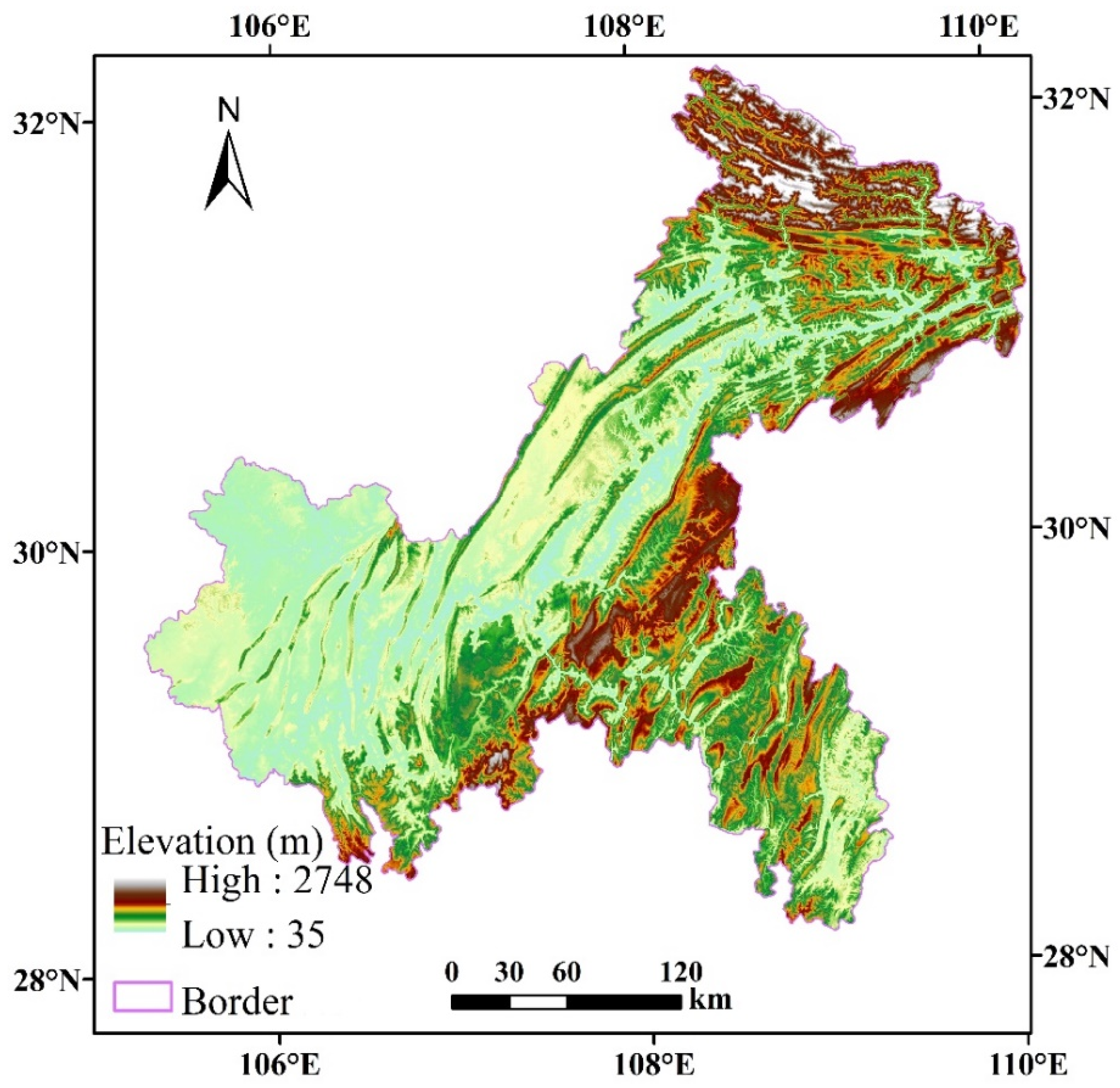
2.1. Study Area
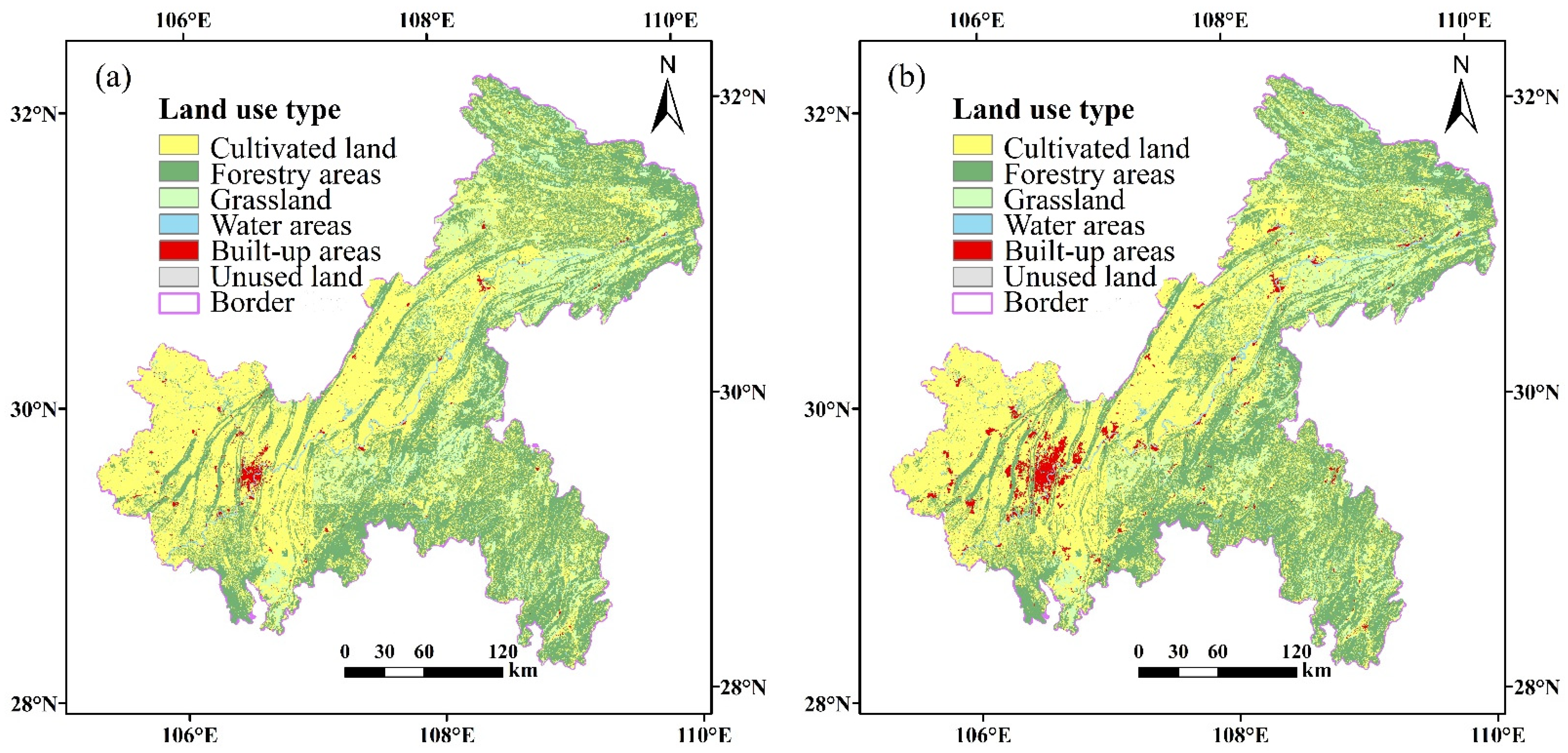
2.2. Data Sources
3. Research Method
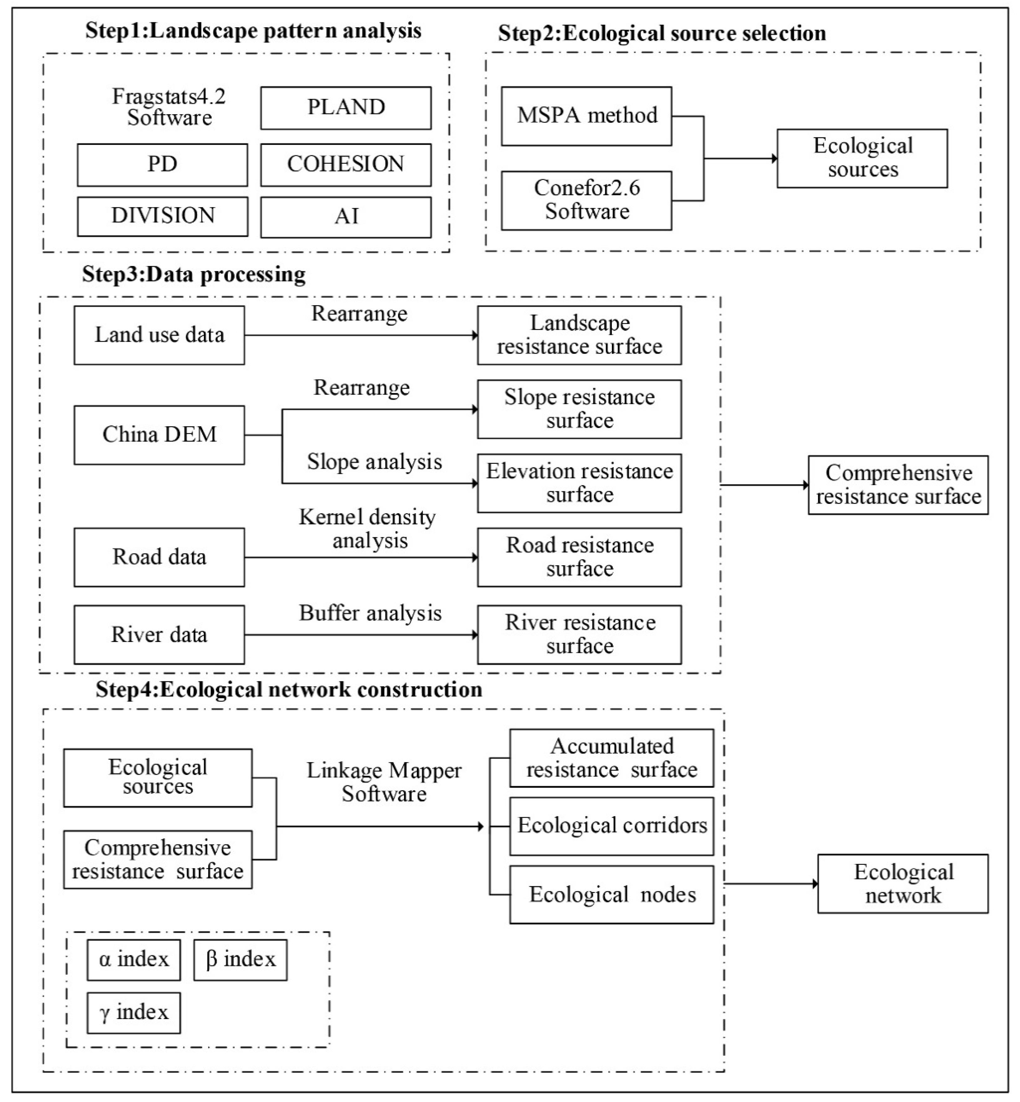
3.1. Technical Route
3.2. Landscape Pattern Index Analysis
3.3. Selection of Ecological Sources
3.3.1. Identification of Core Ecological Patches by the MSPA Method
- Standardized Data Processing
- 2.
- Neighborhood Rule Setting
- 3.
- Edge Width Setting
- 4.
- Generation of Seven Landscape Types
3.3.2. Identification of Ecological Sources by the Landscape Connectivity Index
3.4. Resistance Surface Construction
3.4.1. Construction of Landscape Resistance Surfaces
3.4.2. Construction of the Integrated Resistance Surface
3.4.3. Construction of the Cumulative Resistance Surface
3.5. Minimal Cumulative Resistance Model
3.6. Evaluation of the Ecological Network Index
4. Results and Discussion
4.1. Landscape Pattern Index
4.2. Ecological Source Selection
4.2.1. Identification of Core Ecological Patches
4.2.2. Identification of Ecological Sources
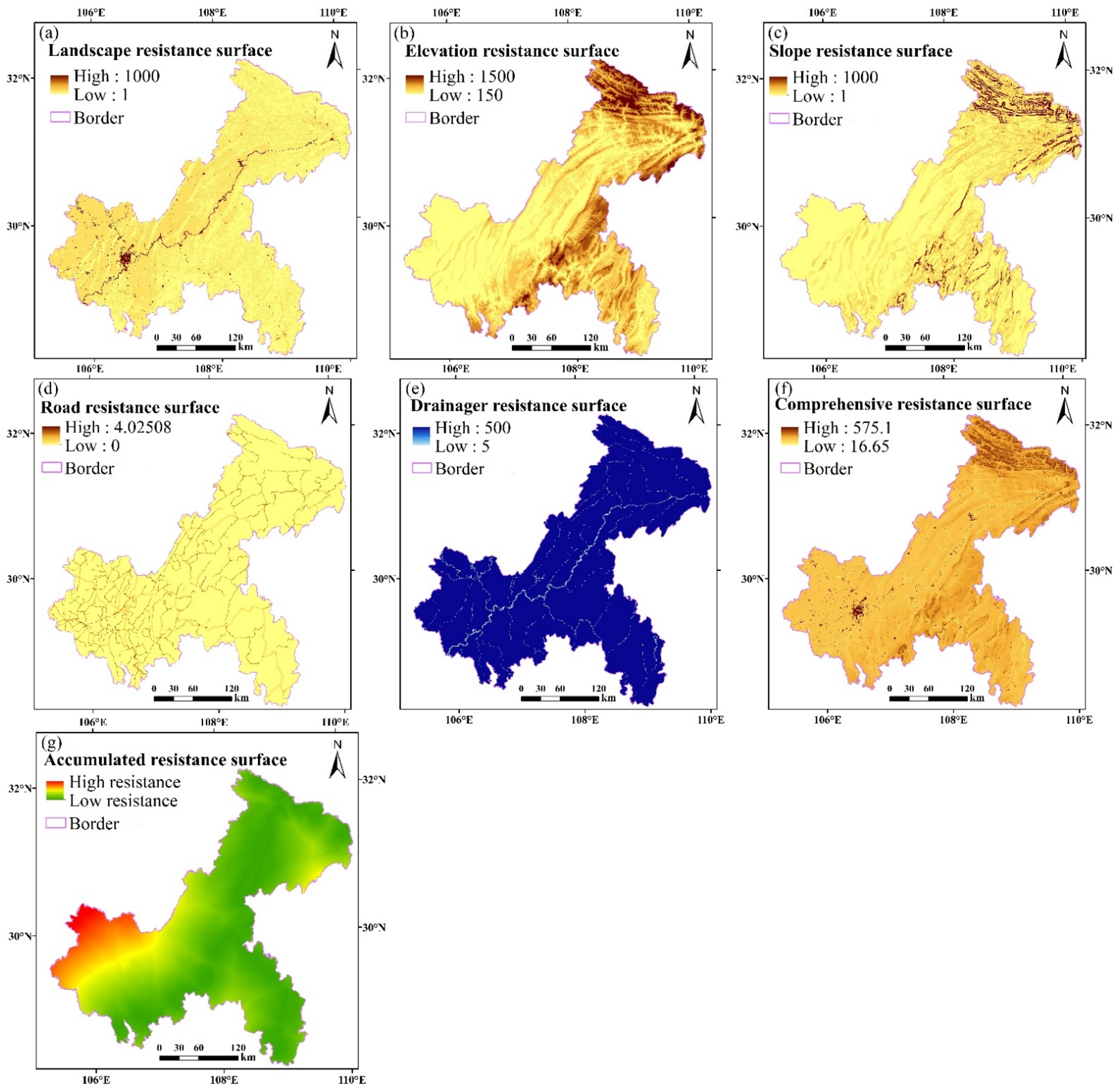
4.3. Resistance Surface Analysis
4.4. Construction of Potential Ecological Corridors in Chongqing
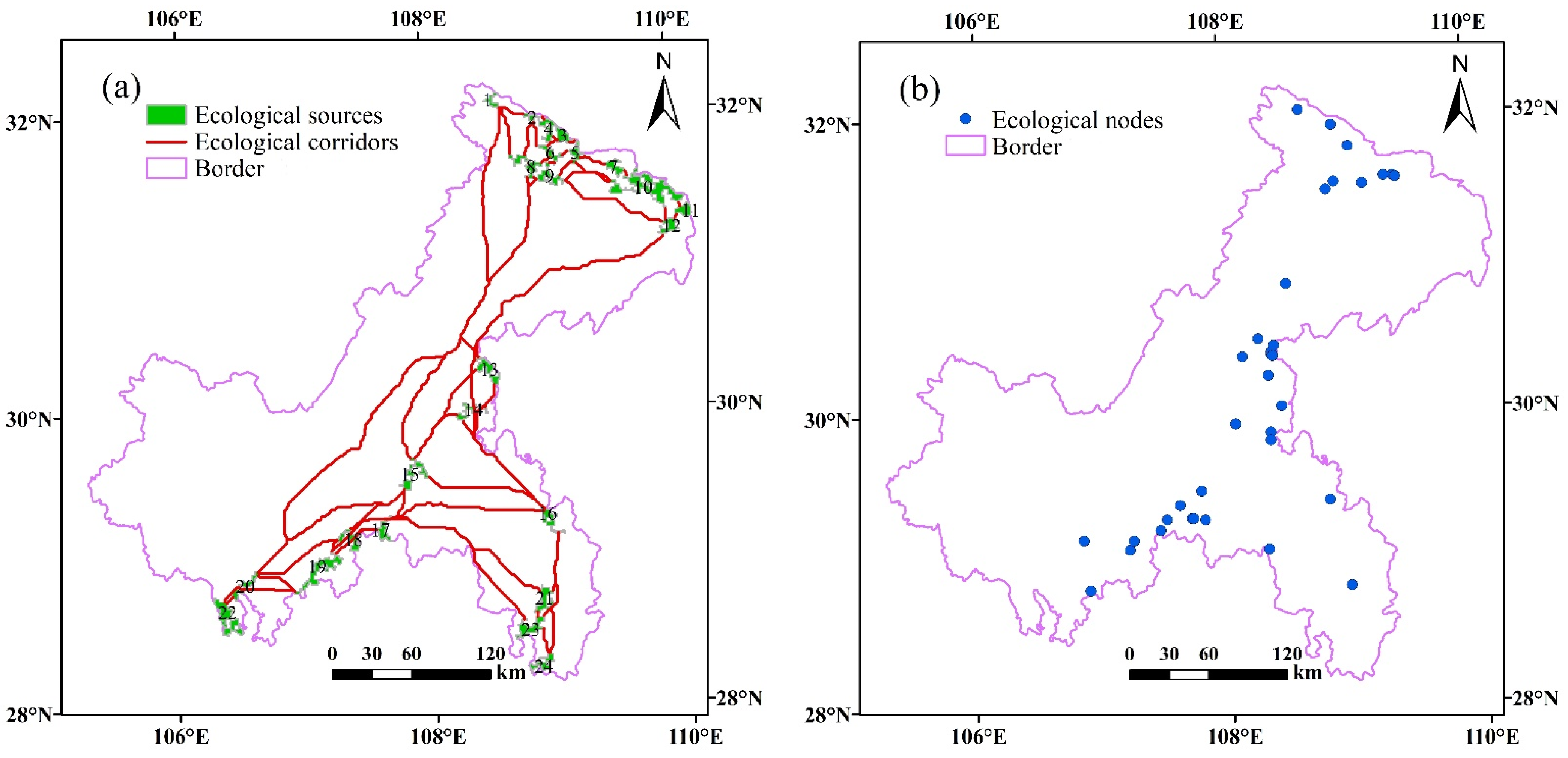
4.4.1. Identification of Potential Ecological Corridors in Chongqing
4.4.2. Ecological Node Identification
4.5. Construction of Chongqing’s Ecological Network
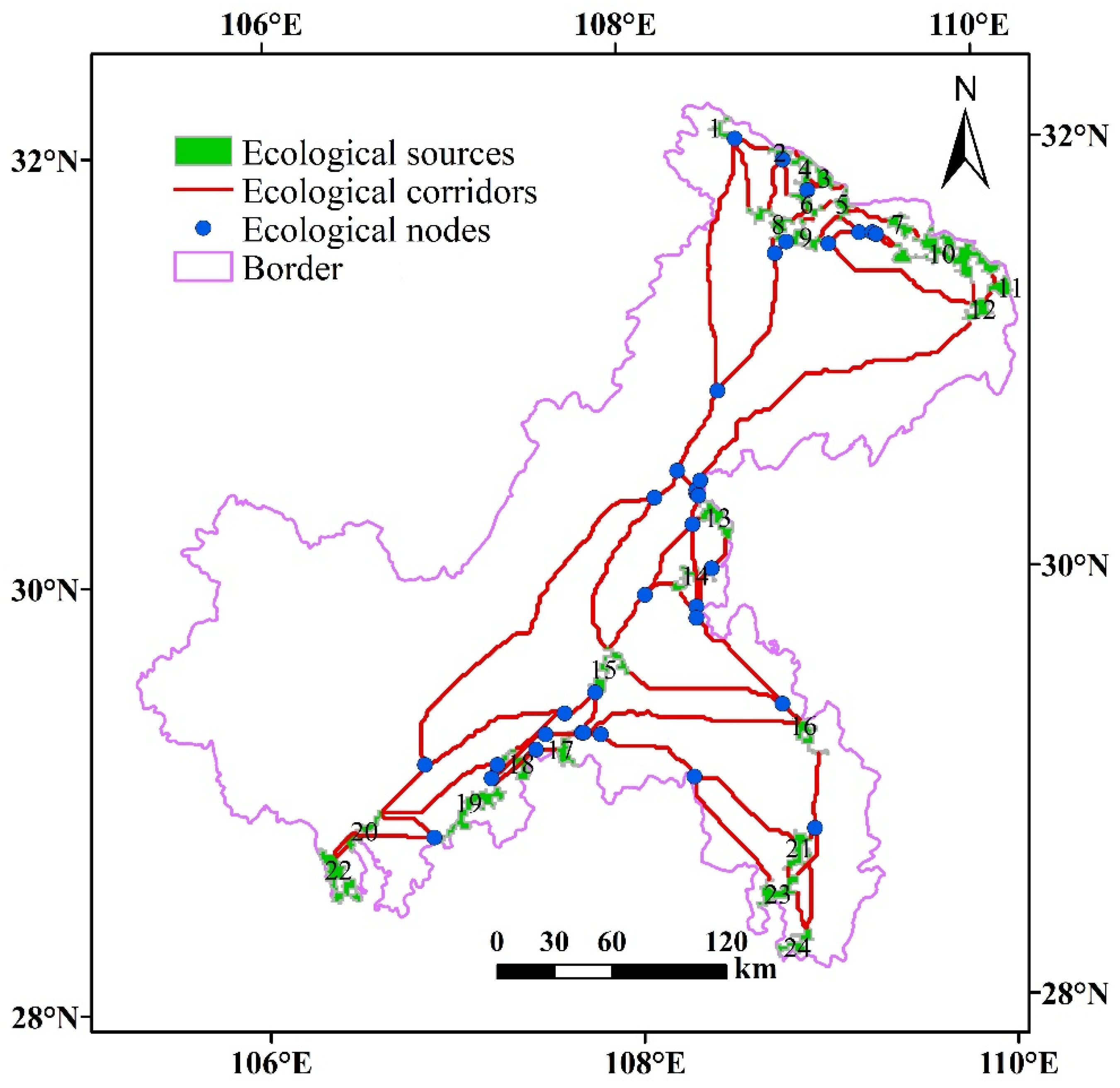
4.5.1. Identification of Chongqing’s Ecological Network
4.5.2. Ecological Network Index Analysis
5. Conclusions
Author Contributions
Funding
Institutional Review Board Statement
Informed Consent Statement
Data Availability Statement
Conflicts of Interest
References
- Song, W.; Pijanowski, B.C. The effects of China’s cultivated land balance program on potential land productivity at a national scale. Appl. Geogr. 2014, 46, 158–170. [Google Scholar] [CrossRef]
- Li, F.; Ye, Y.; Song, B.; Wang, R. Evaluation of urban suitable ecological land based on the minimum cumulative resistance model: A case study from Changzhou, China. Ecol. Model. 2015, 318, 194–203. [Google Scholar] [CrossRef]
- Su, Y.; Chen, X.; Liao, J.; Zhang, H.; Wang, C.; Ye, Y.; Wang, Y. Modeling the optimal ecological security pattern for guiding the urban constructed land expansions. Urban For. Urban Green. 2016, 19, 35–46. [Google Scholar] [CrossRef]
- Carlier, J.; Moran, J. Landscape typology and ecological connectivity assessment to inform Greenway design. Sci. Total Environ. 2019, 651, 3241–3252. [Google Scholar] [CrossRef]
- Song, W.; Deng, X. Land-use/land-cover change and ecosystem service provision in China. Sci. Total Environ. 2017, 576, 705–719. [Google Scholar] [CrossRef]
- Troumbis, A.Y.; Zevgolis, Y. Biodiversity crime and economic crisis: Hidden mechanisms of misuse of ecosystem goods in Greece. Land Use Policy 2020, 99. [Google Scholar] [CrossRef]
- Hugé, J.; de Bisthoven, L.J.; Mushiete, M.; Rochette, A.-J.; Candido, S.; Keunen, H.; Dahdouh-Guebas, F.; Koedam, N.; Vanhove, M.P.M. EIA-driven biodiversity mainstreaming in development cooperation: Confronting expectations and practice in the DR Congo. Environ. Sci. Policy 2020, 104, 107–120. [Google Scholar] [CrossRef]
- Carranza, D.M.; Varas-Belemmi, K.; De Veer, D.; Iglesias-Müller, C.; Coral-Santacruz, D.; Méndez, F.A.; Torres-Lagos, E.; Squeo, F.A.; Gaymer, C.F. Socio-environmental conflicts: An underestimated threat to biodiversity conservation in Chile. Environ. Sci. Policy 2020, 110, 46–59. [Google Scholar] [CrossRef]
- Wang, W.; Feng, C.; Liu, F.; Li, J. Biodiversity conservation in China: A review of recent studies and practices. Environ. Sci. Ecotechnology 2020, 2, 100025. [Google Scholar] [CrossRef]
- McNeely, J.A. The Convention on Biological Diversity. In Encyclopedia of the Anthropocene; Elsevier Inc.: London, UK, 2018; pp. 321–326. [Google Scholar] [CrossRef] [Green Version]
- Chu, E.W.; Karr, J.R. Environmental Impact: Concept, Consequences, Measurement. In Reference Module in Life Sciences; Elsevier BV: Amsterdam, The Netherlands, 2017. [Google Scholar] [CrossRef]
- Wu, X.; Zhang, J.; Geng, X.; Wang, T.; Wang, K.; Liu, S. Increasing green infrastructure-based ecological resilience in urban systems: A perspective from locating ecological and disturbance sources in a resource-based city. Sustain. Cities Soc. 2020, 61. [Google Scholar] [CrossRef]
- Jongman, R. Ecological Networks are an Issue for All of US. J. Landsc. Ecol. 2008. [Google Scholar] [CrossRef] [Green Version]
- Linehan, J.; Gross, M.; Finn, J. Greenway planning: Developing a landscape ecological network approach. Landsc. Urban Plan. 1995, 33. [Google Scholar] [CrossRef]
- An, Y.; Liu, S.; Sun, Y.; Shi, F.; Beazley, R. Construction and optimization of an ecological network based on morphological spatial pattern analysis and circuit theory. Landsc. Ecol. 2020, 1–18. [Google Scholar] [CrossRef]
- De Montis, A.; Ganciu, A.; Cabras, M.; Bardi, A.; Peddio, V.; Caschili, S.; Massa, P.; Cocco, C.; Mulas, M. Resilient ecological networks: A comparative approach. Land Use Policy. 2019, 89, 104207. [Google Scholar] [CrossRef]
- Jongman, R.H.G.; Külvik, M.; Kristiansen, I. European ecological networks and greenways. Landsc. Urban Plan. 2004, 68, 305–319. [Google Scholar] [CrossRef]
- Takemoto, K.; Iida, M. Ecological Networks. In Encyclopedia of Bioinformatics and Computational Biology; Elsevier BV: Amsterdam, The Netherlands, 2019; pp. 1131–1141. [Google Scholar]
- Nor, A.N.M.; Corstanje, R.; Harris, J.A.; Grafius, D.R.; Siriwardena, G.M. Ecological connectivity networks in rapidly expanding cities. Heliyon 2017. [Google Scholar] [CrossRef] [Green Version]
- Yu, Q.; Yue, D.; Wang, Y.; Kai, S.; Fang, M.; Ma, H.; Zhang, Q.; Huang, Y. Optimization of ecological node layout and stability analysis of ecological network in desert oasis: A typical case study of ecological fragile zone located at Deng Kou County(Inner Mongolia). Ecol. Indic. 2018, 84, 304–318. [Google Scholar] [CrossRef]
- Hepcan, Ş.; Hepcan, Ç.C.; Bouwma, I.M.; Jongman, R.H.G.; Özkan, M.B. Ecological networks as a new approach for nature conservation in Turkey: A case study of İzmir Province. Urban Plan. 2009, 90, 143–154. [Google Scholar] [CrossRef]
- Closset-Kopp, D.; Wasof, S.; Decocq, G. Using process-based indicator species to evaluate ecological corridors in fragmented landscapes. Biol. Conserv. 2016, 201, 152–159. [Google Scholar] [CrossRef]
- Peng, J.; Zhao, H.; Liu, Y. Urban ecological corridors construction: A review. Acta Ecol. Sin. 2017, 37, 23–30. [Google Scholar] [CrossRef]
- Jongman, R.H.G. Connectivity and Ecological Networks. In Encyclopedia of Ecology; Elsevier BV: Amsterdam, The Netherlands, 2019; pp. 366–376. [Google Scholar] [CrossRef]
- Shi, F.; Liu, S.; Sun, Y.; An, Y.; Zhao, S.; Liu, Y.; Li, M. Ecological network construction of the heterogeneous agro-pastoral areas in the upper Yellow River basin. Agric. Ecosyst. Environ. 2020, 302, 107069. [Google Scholar] [CrossRef]
- Yang, J.; Zeng, C.; Cheng, Y. Spatial influence of ecological networks on land use intensity. Sci. Total Environ. 2020, 717, 137151. [Google Scholar] [CrossRef] [PubMed]
- Zhang, Y.; Li, X.; Song, W. Determinants of cropland abandonment at the parcel, household and village levels in mountain areas of China: A multi-level analysis. Land Use Policy 2014, 41, 186–192. [Google Scholar] [CrossRef]
- Pili, S.; Serra, P.; Salvati, L. Landscape and the city: Agro-forest systems, land fragmentation and the ecological network in Rome, Italy. Urban For. Urban Green. 2019, 41, 230–237. [Google Scholar] [CrossRef]
- Jordán, F. A reliability-theory approach to corridor design. Ecol. Model. 2000, 128, 211–220. [Google Scholar] [CrossRef]
- Bowers, K.; McKnight, M. Reestablishing a Healthy and Resilient North America—Linking Ecological Restoration with Continental Habitat Connectivity. Ecol. Restor. 2012, 30, 267–270. [Google Scholar] [CrossRef]
- Chettri, N.; Sharma, E.; Shakya, B.; Bajracharya, B. Developing Forested Conservation Corridors in the Kangchenjunga Landscape, Eastern Himalaya. Mt. Res. Dev. 2007, 27, 211–214. [Google Scholar] [CrossRef] [Green Version]
- Su, K.; Yu, Q.; Yue, D.; Zhang, Q.; Yang, L.; Liu, Z.; Niu, T.; Sun, X. Simulation of a forest-grass ecological network in a typical desert oasis based on multiple scenes. Ecol. Model. 2019, 413. [Google Scholar] [CrossRef]
- Aminzadeh, B.; Khansefid, M. A case study of urban ecological networks and a sustainable city: Tehran’s metropolitan area. Urban Ecosyst. 2009, 13, 23–36. [Google Scholar] [CrossRef]
- Zhao, X.Q.; Xu, X.H. Research on landscape ecological security pattern in a Eucalyptus introduced region based on biodiversity conservation. Russ. J. Ecol. 2015, 46, 59–70. [Google Scholar] [CrossRef]
- Wang, C.; Yu, C.; Chen, T.; Feng, Z.; Hu, Y.; Wu, K. Can the establishment of ecological security patterns improve ecological protection? An example of Nanchang, China. Sci. Total Environ. 2020, 740, 140051. [Google Scholar] [CrossRef] [PubMed]
- Dong, J.; Peng, J.; Liu, Y.; Qiu, S.; Han, Y. Integrating spatial continuous wavelet transform and kernel density estimation to identify ecological corridors in megacities. Landsc. Urban Plan. 2020, 199, 103815. [Google Scholar] [CrossRef]
- Liu, S.; Dong, Y.; Cheng, F.; Zhang, Y.; Hou, X.; Dong, S.; Coxixo, A. Effects of road network on Asian elephant habitat and connectivity between the nature reserves in Xishuangbanna, Southwest China. J. Nat. Conserv. 2017, 38, 11–20. [Google Scholar] [CrossRef]
- Pomianowski, W.; Solon, J. Modelling patch mosaic connectivity and ecological corridors with GraphScape. Environ. Model. Softw. 2020, 134, 104757. [Google Scholar] [CrossRef]
- Guo, X.; Zhang, X.; Du, S.; Li, C.; Siu, Y.L.; Rong, Y.; Yang, H. The impact of onshore wind power projects on ecological corridors and landscape connectivity in Shanxi, China. J. Clean. Prod. 2020, 254, 120075. [Google Scholar] [CrossRef]
- Peng, J.; Yang, Y.; Liu, Y.; Hu, Y.; Du, Y.; Meersmans, J.; Qiu, S. Linking ecosystem services and circuit theory to identify ecological security patterns. Sci. Total Environ. 2018, 644, 781–790. [Google Scholar] [CrossRef] [Green Version]
- Dai, L.; Liu, Y.; Luo, X. Integrating the MCR and DOI models to construct an ecological security network for the urban agglomeration around Poyang Lake, China. Sci. Total Environ. 2021, 754, 141868. [Google Scholar] [CrossRef]
- Zhang, Y.; Song, W. Identify Ecological Corridors and Build Potential Ecological Networks in Response to Recent Land Cover Changes in Xinjiang, China. Sustainability 2020, 12, 8960. [Google Scholar] [CrossRef]
- Liu, G.; Yang, Z.; Chen, B.; Zhang, L.; Zhang, Y.; Su, M. An Ecological Network Perspective in Improving Reserve Design and Connectivity: A Case Study of Wuyishan Nature Reserve in China. Ecol. Model. 2015, 306, 185–194. [Google Scholar] [CrossRef]
- Peng, L.; Chen, T.; Liu, S. Spatiotemporal Dynamics and Drivers of Farmland Changes in Panxi Mountainous Region, China. Sustainability 2016, 8, 1209. [Google Scholar] [CrossRef] [Green Version]
- Liang, J.; He, X.; Zeng, G.; Zhong, M.; Gao, X.; Li, X.; Li, X.; Wu, H.; Feng, C.; Xing, W.; et al. Integrating priority areas and ecological corridors into national network for conservation planning in China. Sci. Total Environ. 2018, 626, 22–29. [Google Scholar] [CrossRef]
- Liu, Y.; Yue, W.; Fan, P.; Zhang, Z.; Huang, J. Assessing the urban environmental quality of mountainous cities: A case study in Chongqing, China. Ecol. Indic. 2017, 81, 132–145. [Google Scholar] [CrossRef]
- Huang, L.; Qian, S.; Li, T.; Jim, C.Y.; Jin, C.; Zhao, L.; Lin, D.; Shang, K.; Yang, Y. Masonry walls as sieve of urban plant assemblages and refugia of native species in Chongqing, China. Landsc. Urban Plan. 2019, 191. [Google Scholar] [CrossRef]
- Long, H.; Wu, X.; Wang, W.; Dong, G. Analysis of Urban-Rural Land-Use Change during 1995–2006. Sensors 2008, 8, 681–699. [Google Scholar] [CrossRef] [Green Version]
- Lin, Y.; Li, Y.; Ma, Z. Exploring the Interactive Development between Population Urbanization and Land Urbanization: Evidence from Chongqing, China (1998–2016). Sustainability 2018, 10, 1741. [Google Scholar] [CrossRef] [Green Version]
- Zhang, J.F.; Deng, W. Industrial Structure Change and Its Eco-environmental Influence since the Establishment of Municipality in Chongqing, China. Procedia Environ. Sci. 2010, 2, 517–526. [Google Scholar] [CrossRef] [Green Version]
- Resource Environmental Science and Data Center, Chinese Academy of Sciences. Available online: http://www.resdc.cn/Default.aspx (accessed on 22 November 2020).
- Geospatial Data Cloud Homepage. Availabe online: http://www.gscloud.cn/sources/ (accessed on 22 November 2020).
- Zhang, Q.; Chen, C.; Wang, J.; Yang, D.; Zhang, Y.; Wang, Z.; Gao, M. The spatial granularity effect, changing landscape patterns, and suitable landscape metrics in the Three Gorges Reservoir Area, 1995–2015. Ecol. Indic. 2020, 114, 106259. [Google Scholar] [CrossRef]
- Li, H.; Peng, J.; Yanxu, L.; Yi’na, H. Urbanization impact on landscape patterns in Beijing City, China: A spatial heterogeneity perspective. Ecol. Indic. 2017, 82, 50–60. [Google Scholar] [CrossRef]
- Availabe online: http://www.umass.edu/landeco/research/fragstats/documents/fragstats.help.4.2.pdf (accessed on 22 November 2020).
- Zhang, J.; Qu, M.; Wang, C.; Zhao, J.; Cao, Y. Quantifying landscape pattern and ecosystem service value changes: A case study at the county level in the Chinese Loess Plateau. Glob. Ecol. Conserv. 2020, 23, e01110. [Google Scholar] [CrossRef]
- Vogt, P.; Riitters, K.H.; Iwanowski, M.; Estreguil, C.; Kozak, J.; Soille, P. Mapping landscape corridors. Ecol. Indic. 2007, 7, 481–488. [Google Scholar] [CrossRef]
- Vogt, P.; Riitters, K.H.; Estreguil, C.; Kozak, J.; Wade, T.G.; Wickham, J.D. Mapping Spatial Patterns with Morphological Image Processing. Landsc. Ecol. 2006, 22, 171–177. [Google Scholar] [CrossRef]
- Wang, J.; Xu, C.; Pauleit, S.; Kindler, A.; Banzhaf, E. Spatial patterns of urban green infrastructure for equity: A novel exploration. J. Clean. Prod. 2019, 238, 238. [Google Scholar] [CrossRef]
- Zhang, Y.; Shen, W.; Li, M.; Lv, Y. Assessing spatio-temporal changes in forest cover and fragmentation under urban expansion in Nanjing, eastern China, from long-term Landsat observations (1987–2017). Appl. Geogr. 2020, 117, 102190. [Google Scholar] [CrossRef]
- Cui, L.; Wang, J.; Sun, L.; Lv, C. Construction and optimization of green space ecological networks in urban fringe areas: A case study with the urban fringe area of Tongzhou district in Beijing. J. Clean. Prod. 2020, 276, 124266. [Google Scholar] [CrossRef]
- Rosot, M.A.D.; Maran, J.C.; de Luz, N.B.; Garrastazú, M.C.; de Oliveira, Y.M.M.; Franciscon, L.; Clerici, N.; Vogt, P.; de Freitas, J.V. Riparian forest corridors: A prioritization analysis to the Landscape Sample Units of the Brazilian National Forest Inventory. Ecol. Indic. 2018, 93, 501–511. [Google Scholar] [CrossRef]
- Hernando, A.; Velázquez, J.; Valbuena, R.; Legrand, M.; García-Abril, A. Influence of the resolution of forest cover maps in evaluating fragmentation and connectivity to assess habitat conservation status. Ecol. Indic. 2017, 79, 295–302. [Google Scholar] [CrossRef]
- Saura, S.; Pascual-Hortal, L. A new habitat availability index to integrate connectivity in landscape conservation planning: Comparison with existing indices and application to a case study. Landsc. Urban Plan. 2007, 83, 91–103. [Google Scholar] [CrossRef]
- Ye, H.; Yang, Z.; Xu, X. Ecological Corridors Analysis Based on MSPA and MCR Model—A Case Study of the Tomur World Natural Heritage Region. Sustainability 2020, 12, 959. [Google Scholar] [CrossRef] [Green Version]
- Pascual-Hortal, L.; Saura, S. Comparison and development of new graph-based landscape connectivity indices: Towards the priorization of habitat patches and corridors for conservation. Landsc. Ecol. 2006, 21, 959–967. [Google Scholar] [CrossRef]
- Zeller, K.A.; McGarigal, K.; Whiteley, A.R. Estimating landscape resistance to movement: A review. Landsc. Ecol. 2012, 27, 777–797. [Google Scholar] [CrossRef]
- Jewitt, D.; Goodman, P.S.; Erasmus, B.F.; O’Connor, T.G.; Witkowski, E.T. Planning for the Maintenance of Floristic Diversity in the Face of Land Cover and Climate Change. Environ. Manag. 2017, 59, 792–806. [Google Scholar] [CrossRef] [PubMed]
- Jan, P.K.; Marten, S.; Bert, H. Estimating habitat isolation in landscape planning. Landsc. Urban Plan. 1992, 23, 1–16. [Google Scholar]
- Yu, K.J. Security patterns and surface model in landscape ecological planning. Landsc. Urban Plan. 1996, 36, 1–17. [Google Scholar] [CrossRef]
- Shi, H.; Shi, T.; Yang, Z.; Wang, Z.; Han, F.; Wang, C. Effect of Roads on Ecological Corridors Used for Wildlife Movement in a Natural Heritage Site. Sustainability 2018, 10, 2725. [Google Scholar] [CrossRef] [Green Version]
- Li, H.; Chen, W.; He, W. Planning of Green Space Ecological Network in Urban Areas: An Example of Nanchang, China. Int. J. Environ. Res. Public Health 2015, 12, 12889–12904. [Google Scholar] [CrossRef] [Green Version]
- Grêt-Regamey, A.; Weibel, B. Global assessment of mountain ecosystem services using earth observation data. Ecosyst. Serv. 2020, 46, 101213. [Google Scholar] [CrossRef]
- Miao, Z.; Pan, L.; Wang, Q.; Chen, P.; Yan, C.; Liu, L. Research on Urban Ecological Network Under the Threat of Road Networks—A Case Study of Wuhan. ISPRS Int. Geo-Inf. 2019, 8, 342. [Google Scholar] [CrossRef] [Green Version]
- Yang, C.; Zeng, W.; Yang, X. Coupling coordination evaluation and sustainable development pattern of geo-ecological environment and urbanization in Chongqing municipality, China. Sustain. Cities Soc. 2020, 61, 102271. [Google Scholar] [CrossRef]


| Resistance Factors | Weight | Classification Indicators | Resistance Value |
|---|---|---|---|
| Land use types | 0.30 | Forests | 1 |
| Shrubs, sparse forests | 3 | ||
| Paddy fields, dry lands | 50 | ||
| Other forestry areas | 300 | ||
| High-coverage grassland | 10 | ||
| Medium-cover grassland | 15 | ||
| Low-coverage grassland | 20 | ||
| Rivers | 600 | ||
| Lakes | 300 | ||
| Reservoir Pit Tong | 100 | ||
| Beach | 1 | ||
| Urban land, rural settlements | 900 | ||
| Other construction sites | 1000 | ||
| Others | 700 | ||
| Elevation | 0.10 | Elevation range | Resistance value |
| <450 m | 150 | ||
| 450–700 m | 300 | ||
| 700–1000 m | 500 | ||
| 1000–1400 m | 800 | ||
| 1400–1800 m | 1000 | ||
| >1800 m | 1500 | ||
| Slope | 0.10 | Slope range | Resistance value |
| <3° | 1 | ||
| 3–6° | 20 | ||
| 6–10° | 100 | ||
| 10–16° | 200 | ||
| >16° | 600 | ||
| Roads | 0.25 | Road types | Resistance value |
| Railways | 700 | ||
| National Highway | 2000 | ||
| Other roads | 500 | ||
| Rivers | 0.25 | Buffer | Resistance value |
| Level I rivers | <50 m | 5 | |
| 50–120 m | 25 | ||
| 120–300 m | 50 | ||
| Level II rivers | <50 m | 10 | |
| 50–120 m | 50 | ||
| 120–300 m | 100 | ||
| Level III rivers | <50 m | 20 | |
| 50–120 m | 100 | ||
| 120–300 m | 500 |
| Landscape Index | Year | Cultivated Land | Forestland | Grassland | Water Areas | Built-Up Areas | Unused Land |
|---|---|---|---|---|---|---|---|
| PLAND (100%) | 2005 | 46.49 | 40.45 | 11.00 | 1.16 | 0.88 | 0.02 |
| 2015 | 45.61 | 41.01 | 9.54 | 1.45 | 2.38 | 0.01 | |
| PD (n/ha) | 2005 | 0.31 | 0.15 | 0.08 | 0.01 | 0.02 | 0.00 |
| 2015 | 0.30 | 0.15 | 0.08 | 0.01 | 0.04 | 0.00 | |
| COHESION | 2005 | 99.83 | 99.95 | 99.47 | 99.77 | 98.32 | 93.23 |
| 2015 | 99.84 | 99.95 | 99.10 | 99.81 | 98.84 | 93.01 | |
| DIVISION | 2005 | 0.98 | 0.98 | 1.00 | 1.00 | 1.00 | 1.00 |
| 2015 | 0.98 | 0.97 | 1.00 | 1.00 | 1.00 | 1.00 | |
| AI | 2005 | 94.84 | 95.08 | 92.66 | 93.73 | 93.34 | 87.19 |
| 2015 | 94.87 | 95.15 | 92.59 | 94.09 | 95.21 | 86.64 |
| Index | L | V | L − V + 1 | 2V − 5 | 3 (V − 2) | Results | |
|---|---|---|---|---|---|---|---|
| Ecological Network | α index | 87 | 35 | 53 | 65 | 0.82 | |
| β index | 87 | 35 | 2.49 | ||||
| γ index | 87 | 35 | 99 | 0.89 |
Publisher’s Note: MDPI stays neutral with regard to jurisdictional claims in published maps and institutional affiliations. |
© 2021 by the authors. Licensee MDPI, Basel, Switzerland. This article is an open access article distributed under the terms and conditions of the Creative Commons Attribution (CC BY) license (https://creativecommons.org/licenses/by/4.0/).
Share and Cite
Zhou, D.; Song, W. Identifying Ecological Corridors and Networks in Mountainous Areas. Int. J. Environ. Res. Public Health 2021, 18, 4797. https://doi.org/10.3390/ijerph18094797
Zhou D, Song W. Identifying Ecological Corridors and Networks in Mountainous Areas. International Journal of Environmental Research and Public Health. 2021; 18(9):4797. https://doi.org/10.3390/ijerph18094797
Chicago/Turabian StyleZhou, Di, and Wei Song. 2021. "Identifying Ecological Corridors and Networks in Mountainous Areas" International Journal of Environmental Research and Public Health 18, no. 9: 4797. https://doi.org/10.3390/ijerph18094797