
Local Disproportions of Quality of Life and Their Influence on the Process of Green Economy Development in Polish Voivodships in 2010–2020


Abstract
:1. Introduction
2. Literature Review
3. Materials and Methods
- maxxij—maximum value of the j-th variable,
- minxij—minimum value of the j-th variable,
- xij—is the value of the j-th variable for this object,
- (a)
- for the pattern:
- (b)
- for the antipattern:
- (a)
- distances of objects from the pattern:
- (b)
- distances of objects from the antipattern:
- b—is the regression coefficient calculated for the individual variables of the model;
- x—explanatory variable;
- y—is the dependent variable;
- a—is an intercept.
- n—number of spatial objects (number of points or polygons);
- xi, xj—values of the variable for the compared objects;
- —average value of the variable for all objects;
- wij—elements of the spatial weight matrix (weights matrix standardized with rows to one),
- so= ,
- σ2 = ,—variance [95].
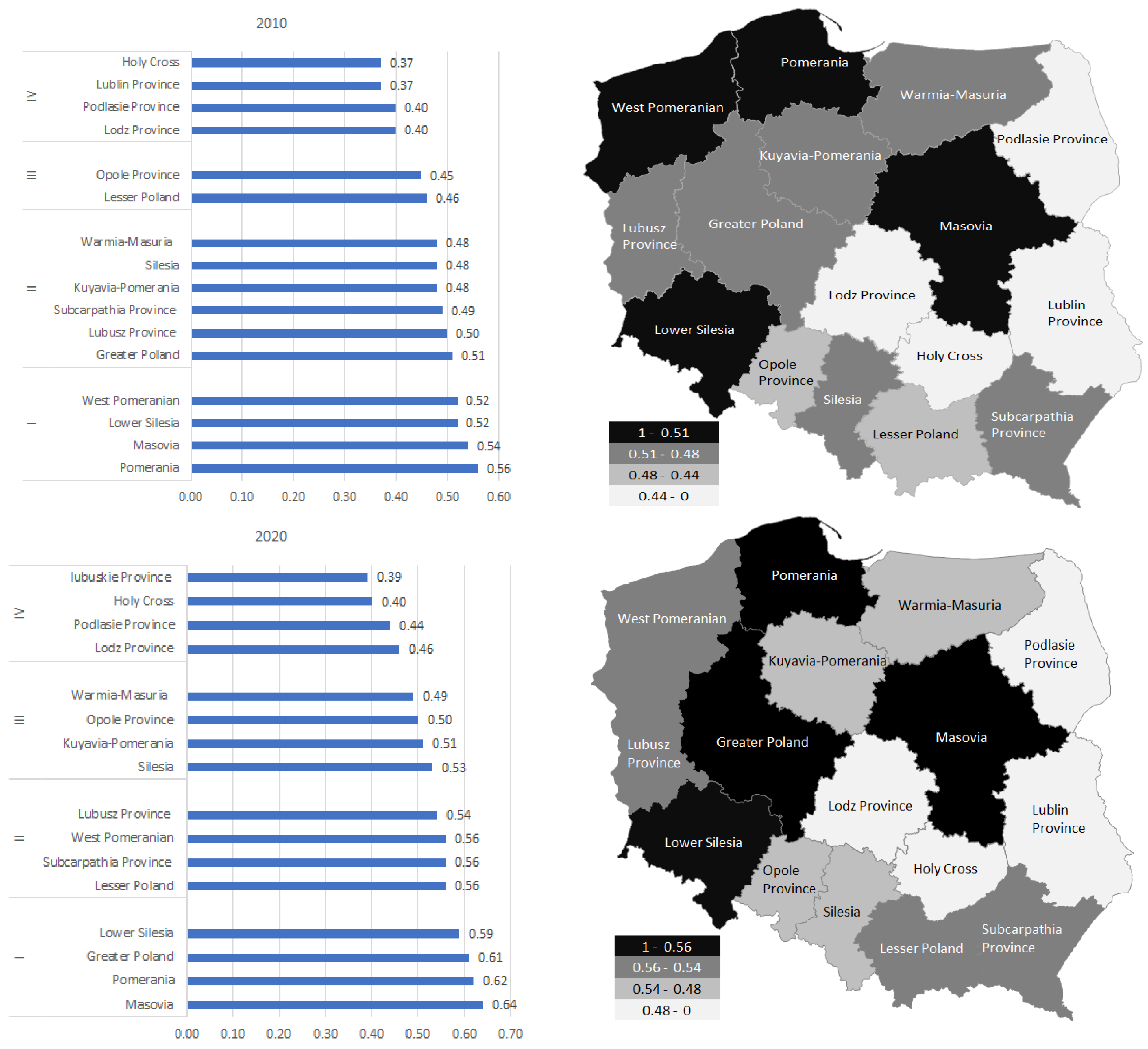
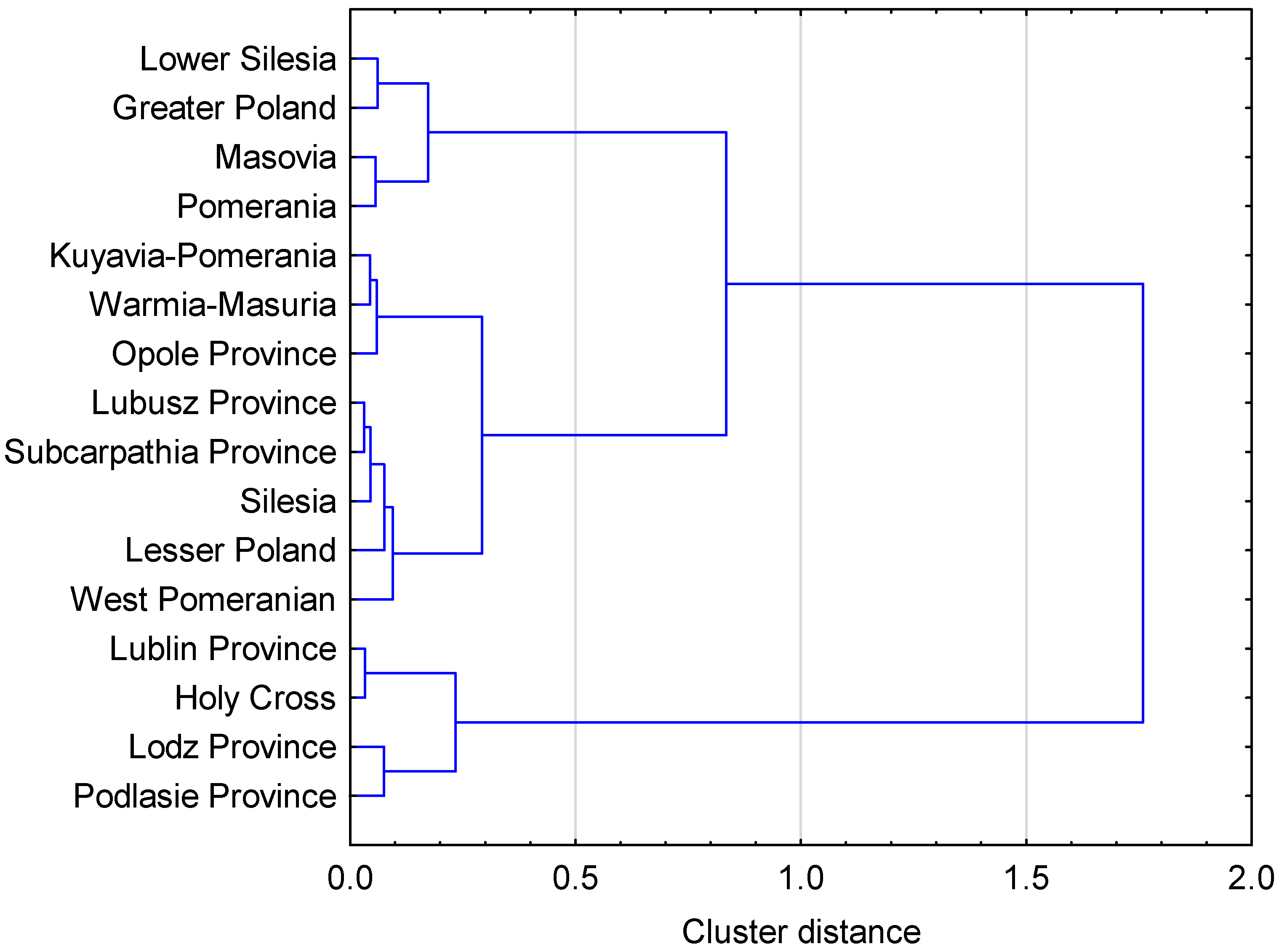
4. Results
- Group I: Lower Silesia, Greater Poland, Masovia, and Pomerania (the group includes units with the highest level of synthesis and the best sizes of diagnostic plots);
- Group II: Kuyavian-Pomeranian, Warmian-Masurian, Opole Province, Lubusz, Subcarpathian, Silesian, Lesser Poland, and West Pomeranian;
- Group III: Lublin Province, Holy Cross, Lodz Province, and Podlasie Province (Figure 4).
5. Discussion
6. Conclusions
Author Contributions
Funding
Institutional Review Board Statement
Informed Consent Statement
Data Availability Statement
Conflicts of Interest
References
- Krugman, P. The Return of Depression Economics and the Crisis of 2008; W.W. Norton & Company: New York, NY, USA; London, UK, 2009. [Google Scholar]
- Gorzelak, G. Geografia Polskiego Kryzysu. Kryzys Peryferii czy Peryferia Kryzysu? RSA—Sekcja Polska: Warszawa, Poland, 2009. [Google Scholar]
- Gorzelak, G. Kryzys finansowy w krajach Europy Środkowej i Wschodniej. In Europejskie Wyzwania dla Polski i jej Regionów; Tucholska, A., Ed.; Ministerstwo Rozwoju Regionalnego: Warszawa, Poland, 2010. [Google Scholar]
- Heshmati, A. An Empirical Survey of the Ramifications of a Green Economy; IZA Discussion Papers, No. 8078; Institute for the Study of Labor (IZA): Bonn, Germany, 2014. [Google Scholar]
- Binda, J.; Łapińska, H. The 2030 Agenda for Sustainable Development and improvements in quality of life in Poland. ASEJ Sci. J. Bielsk. Sch. Financ. Law 2019, 22, 13–16. [Google Scholar] [CrossRef]
- Kryk, B. Środowiskowe uwarunkowania jakości życia w województwie zachodniopomorskim na tle Polski. Ekon. Sr. 2015, 3, 170–181. [Google Scholar]
- Piasny, J. Poziom i jakość życia ludności oraz źródła i mierniki ich określania. Ruch Praw. Ekon. Socjol. 1993, 2, 73–92. [Google Scholar]
- Drewnowski, J.; Scott, W. The Level of Living Index; Report No. 4; UNRISD: Geneva, Switzerland, 1966. [Google Scholar]
- Towards a Green Economy: Pathways to Sustainable Development and Poverty Eradication—A Synthesis for Policy Makers 2011 (2012), United Nations Environmental Programm. Available online: www.unep.org/greeneconomy (accessed on 1 March 2022).
- Kasztelan, A. Zielony wzrost jako nowy kierunek rozwoju gospodarki w warunkach zagrożeń ekologicznych. Stud. Ekon. 2015, 2, 185–208. [Google Scholar]
- Loiseau, E.; Saikku, L.; Antikainen, R.; Droste, N.; Hansjürgens, B.; Pitkänen, K.; Leskinen, P.; Kuikman, P.; Thomsen, M. Green economy and related concepts: An overview. J. Clean. Prod. 2016, 139, 361–371. [Google Scholar] [CrossRef]
- Ryszawska, B. Zielona gospodarka w dokumentach strategicznych Unii Europejskiej. Ekon. Sr. 2013, 3, 26–37. [Google Scholar]
- UN Conference RIO+20, Contribution by the European Union and Its Member States, United Nations Conference on Sustainable Development 2012. Available online: www.unep.org (accessed on 1 March 2022).
- Venkata Mohan, S.; Nikhil, G.N.; Chiranjeevi, P.; Nagendranatha Reddy, C.; Rohit, M.V.; Kumar, A.N.; Sarkar, O. Modele biorafinerii odpadów w kierunku zrównoważonej biogospodarki o obiegu zamkniętym: Krytyczny przegląd i perspektywy na przyszłość. Bioresour. Technol. 2016, 215, 2–12. [Google Scholar] [CrossRef]
- Venkata Mohan, S.; Modestra, J.A.; Amulya, K.; Butti, S.K.; Velvizhi, G. Biogospodarka o obiegu zamkniętym z bioproduktami z sekwestracji CO2. Trendy Biotechnol. 2016, 34. [Google Scholar]
- OECD. Applications of Complexity Science for Public Policy; OECD: Paris, France, 2009. [Google Scholar]
- Sterman, J.D. Sustaining Sustainability: Creating a Systems Science in a Fragmented Academy and Polarized World. Springer Science+Business Media. Available online: http://jsterman.scripts.mit.edu/docs/Sterman%20Sustaining%20Sustainability%2010-2.pdf (accessed on 1 March 2022).
- Ostasiewicz, W. Ocena i Analiza Jakości Życia; Wydaw, A.E., Ed.; Wydawnictwo Akademii Ekonomicznej we Wrocławiu: Wrocław, Poland, 2004. [Google Scholar]
- Borys, T.; Rogala, P. Jakość Życia na Poziomie Lokalnym—Ujęcie Wskaźnikowe; Program Narodów Zjednoczonych ds. Rozwoju (UNDP) w Polsce: Warszawa, Poland, 2008. [Google Scholar]
- Kusterka-Jefmańska, M. Jakość życia a procesy zarządzania rozwojem lokalnym. Pr. Nauk. Uniw. Ekon. Wrocławiu 2015, 391, 202–210. [Google Scholar] [CrossRef]
- Romney, D.M. A Structural Analysis of Health Related Quality of Life Dimensuins. Hum. Relat. 2002, 45, 165–176. [Google Scholar] [CrossRef]
- Enãchescu, V.; Hristache, D.A.; Paicu, C. The interpretative valences of the relationship between sustainable development and the quality of life. Rev. Appl. Socio-Econ. Res. 2012, 4, 93–96. [Google Scholar]
- Van de Kerk, G.; Manuel, A.R. A comprehensive index for a sustainable society: The SSI—The Sustainable Society Index. Ecol. Econ. 2008, 66, 228–242. [Google Scholar] [CrossRef]
- Berbeka, J. Jakość życia ludności w województwie małopolskim: Ocena subiektywna. Zesz. Nauk. Akad. Ekon. Krakowie 2005, 697, 17–28. [Google Scholar]
- Zborowski, A. Przemiany Struktury Społeczno-Przestrzennej Regionu Miejskiego w Okresie Realnego Socjalizmu i Transformacji Ustrojowej (na Przykładzie Krakowa); Instytut Geografii i Gospodarki Przestrzennej UJ: Kraków, Poland, 2005. [Google Scholar]
- Sobala-Gwosdz, A. Poziom życia w miastach województwa podkarpackiego a ich położenie, funkcje i pozycja w hierarchii. In Zróżnicowanie Warunków Życia Ludności w Mieście, Konwersatorium Wiedzy o Mieście; Jażdżewska, I., Ed.; Wydawnictwo Uniwersytetu Łódzkiego: Łódź, Poland, 2004; pp. 107–120. [Google Scholar]
- Gotowska, M.; Jakubczak, J. Zastosowanie wybranych metod do oceny zróżnicowania poziomu życia ludności w Polsce. In Modele Ustroju Społecnzo-Gospodarczego; Kontrowersje i Dylematy; Mączynska, E., Ed.; PTE: Warszawa, Poland, 2015. [Google Scholar]
- Rutkowski, J. Jak badać jakość życia. Wiadomości Statystyczne 1988, 5, 42. [Google Scholar]
- Kud, K.; Woźniak, M. Percepcja środowiskowych czynników jakości życia na obszarach wiejskich w województwie podkarpackim. Humanit. Soc. Sci. 2013, 18, 63–74. [Google Scholar] [CrossRef]
- Kusterka-Jefmańska, M. Wysoka jakość życia jako cel nadrzędny lokalnych strategii zrównoważonego rozwoju, Zarządzanie publiczne. Zesz. Nauk. Inst. Spraw. Publicznych Uniw. Jagiellońskiego 2010, 12, 115–123. [Google Scholar]
- Kusterka-Jefmańska, M. Pomiar jakości życia na poziomie lokalnym—Wybrane doświadczenia europejskie i doświadczenia polskich samorządów. Pr. Nauk. Uniw. Ekon. Wrocławiu 2012, 264, 230–239. [Google Scholar]
- Štreimikienė, D. Quality of Life and Housing. Int. J. Inf. Educ. Technol. 2015, 5, 140–145. [Google Scholar]
- Papuć, E. Jakość życia—Definicje i sposoby jej ujmowania. Curr. Probl. Psychiatry 2011, 12, 141–145. [Google Scholar]
- Rogala, P. Pomiar subiektywnej jakości życia na poziomie lokalnym—Studium przypadku. Ekon. Wroc. Econ. Rev. 2017, 23, 35–43. [Google Scholar] [CrossRef] [Green Version]
- Borys, T. Jakość Życia Jako Integrujący Rodzaj Jakości, w: Jakość Życia w Perspektywie Nauk Humanistycznych, Ekonomicznych i Ekologii; Akademia Ekonomiczna we Wrocławiu: Jelenia Góra, Poland, 2003. [Google Scholar]
- D’Amato, D.; Korhonen, J. Integrating the green economy, circular economy and bioeconomy in a strategic sustainability framework. Ecol. Econ. 2021, 188, 107143. [Google Scholar] [CrossRef]
- Kuzior, A.; Arefieva, O.; Poberezhna, Z.; Ihumentsev, O. The Mechanism of Forming the Strategic Potential of an Enterprise in a Circular Economy. Sustainability 2022, 14, 3258. [Google Scholar] [CrossRef]
- Ghisellini, P.; Cialani, C.; Ulgiati, S. A review on circular economy: The expected transition to a balanced interplay of environmental and economic systems. J. Clean. Prod. 2016, 114, 11–32. [Google Scholar] [CrossRef]
- Murray, A.; Skene, K.; Haynes, K. The circular economy: An interdisciplinary exploration of the concept and application in a global context. J. Bus. Ethics 2017, 140, 369–380. [Google Scholar] [CrossRef] [Green Version]
- Strahl, D. Możliwości wykorzystania miar agregatowych do oceny konkurencyjności regionów. Pr. Nauk. Wrocławiu 2000, 860, 106–120. [Google Scholar]
- Szulc, E. Ekonometryczna Analiza Wielowymiarowych Procesów Gospodarczych; Wydawnictwo UMK: Toruń, Poland, 2007. [Google Scholar]
- Kukuła, K. Metoda Unitaryzacji Zerowanej; s. 86. Powtórka; PWN: Warszawa, Poland, 2000. [Google Scholar]
- Malina, A. Wielowymiarowa Analiza Przestrzennego Zróżnicowania Struktury Gospodarki Polski Według Województw; Wyd. Akademii Ekonomicznej w Krakowie: Kraków, Poalnd, 2004; pp. 96–97. [Google Scholar]
- Kukuła, K.; Luty, L. O wyborze metody porządkowania liniowego do oceny gospodarki odpadami w Polsce w ujęciu przestrzennym. Zesz. Nauk. Szkoły Głównej Gospod. Wiej. Warszawie 2018, 18, 183–192. [Google Scholar] [CrossRef] [Green Version]
- Malina, A.; Zeliaś, A. O Budowie Taksonomicznej Miary Jakości Życia, Taksonomia 4; Wydawnictwo Akademii Ekonomicznej we Wrocławiu: Wrocław, Polska, 1997. [Google Scholar]
- Sobczak, E. Klasyfikacja podregionów Polski ze względu na stopień ochrony środowiska. Pr. Nauk. Akad. Ekon. Wrocławiu 2004, 1009, 107–119. [Google Scholar]
- Czyż, T. Zastosowanie metody czynnikowej w badaniach przestrzenno-ekonomicznych. Przegląd Geogr. 1970, 42, 467–486. [Google Scholar]
- Adamowicz, M.; Janulewicz, P. Wykorzystanie analizy czynnikowej do oceny rozwoju społeczno-gospodarczego w skali lokalnej. Pr. Nauk. Uniw. Ekon. Wrocławiu 2013, 305, 15–23. [Google Scholar]
- Malina, A. Analiza czynnikowa jako metoda klasyfikacji regionów Polski. Przegląd Stat. 2006, 53, 33–48. [Google Scholar]
- Wysocki, F. Metody Taksonomiczne w Rozpoznawaniu Typów Ekonomicznych Rolnictwa i Obszarów Wiejskich; Wyd. Uniwersytetu Przyrodniczego w Poznaniu: Poznań, Poalnd, 2010. [Google Scholar]
- Łuczak, A.; Wysocki, F. Wykorzystanie Metod Taksonometrycznych i Analitycznego Procesu Hierarchicznego do Programowania Rozwoju Obszarów Wiejskich; Wydawnictwo Akademii Rolniczej im. Augusta Cieszkowskiego w Poznaniu: Poznań, Poland, 2005. [Google Scholar]
- Grabiński, T. Metody określania charakteru zmiennych w wielowymiarowej analizie porównawczej. Zesz. Nauk. Akad. Ekon. Krakowie 1985, 213, 35–63. [Google Scholar]
- Pluta, W. Wielowymiarowa Analiza Porównawcza w Badaniach Ekonometrycznych; PWN: Warszawa, Poland, 1986. [Google Scholar]
- Walesiak, M. Problemy selekcji i ważenia zmiennych w zagadnieniu klasyfikacji. Pr. Nauk. Wroc. Taksonomia 2005, 12, 106–118. [Google Scholar]
- Rogowski, W.; Krysiak, N. Zastosowanie metody wzorca do tworzenia klas ryzyka kredytowego. Bank Kredyt 1997, 7–8, 92–103. [Google Scholar]
- Hellwig, Z.; Siedlecka, U.; Siedlecki, U. Taksonometryczne Modele Zmian Struktury Gospodarczej Polski; Instytut Rozwoju i Studiów Strategicznych: Warszawa, Poland, 1995; p. 16. [Google Scholar]
- Özkan, B.; Özceylan, E.; Kabak, M.; Dikmen, A.U. Evaluation of criteria and COVID-19 patients for intensive care unit admission in the era of pandemic: A multi-criteria decision making approach. Comput. Methods Programs Biomed. 2021, 209, 106348. [Google Scholar] [CrossRef]
- Hellwig, Z. Taksonometria ekonomiczna, jej osiągnięcia, zadania i cele. In Taksonomia–Teoria i jej Zastosowania; Pociecha, J., Ed.; Wydawnictwo Akademii Ekonomicznej w Krakowie: Kraków, Poland, 1990. [Google Scholar]
- Wysocki, F.; Lira, J. Statystyka Opisowa; Wyd. AR: Poznań, Poland, 2005. [Google Scholar]
- Młodak, A. Analiza Taksonomiczna w Statystyce Regionalnej; Centrum Doradztwa i Informacji Difin: Warszawa, Poland, 2006. [Google Scholar]
- Prus, P.; Dziekański, P.; Bogusz, M.; Szczepanek, M. Spatial Differentiation of Agricultural Potential and the Level of Development of Voivodeships in Poland in 2008–2018. Agriculture 2021, 11, 229. [Google Scholar] [CrossRef]
- Dziekanski, P.; Pawlik, A.; Wronska, M.; Karpinska, U. Demographic Potential as the Basis for Spatial Differentiation of the Financial Situation Communes of Eastern Poland in 2009-2018. Eur. Res. Stud. J. 2020, 23, 872–892. [Google Scholar] [CrossRef]
- Dziekański, P.; Prus, P. Financial Diversity and the Development Process: Case study of Rural Communes of Eastern Poland in 2009–2018. Sustainability 2020, 12, 6446. [Google Scholar] [CrossRef]
- Lenormand, M.; Deffuant, G. Generating a Synthetic Population of Individuals in Households: Sample-Free vs Sample-Based Methods. J. Artif. Soc. Soc. Simul. 2013, 6, 1–12. [Google Scholar] [CrossRef]
- Malina, A. Analiza przestrzennego zróżnicowania poziomu rozwoju społeczno-gospodarczego województw Polski w latach 2005–2017. Nierówności Społeczne Wzrost Gospod. 2020, 61, 138–155. [Google Scholar] [CrossRef]
- Hellwig, Z. Zastosowanie metody taksonomicznej do typologicznego podziału krajów ze względu na poziom ich rozwoju oraz zasoby i strukturę wykwalifikowanych kadr. Przegląd Stat. 1968, 4, 307–326. [Google Scholar]
- Wójcik-Leń, J.; Leń, P.; Mika, M.; Kryszk, H.; Kotlarz, P. Studies regarding correct selection of statistical methods for the needs of increasing the efficiency of identification of land for consolidation—A case study in Poland. Land Use Policy 2000, 87, 104064. [Google Scholar] [CrossRef]
- Bąk, A. Zastosowanie metod wielowymiarowej analizy porównawczej do oceny stanu środowiska w województwie dolnośląskim. Wiad. Stat. 2018, 63, 7–20. [Google Scholar]
- Behzadian, M.; Khanmohammadi Otaghsara, S.; Yazdani, M.; Ignatius, J. A state-of the-art survey of TOPSIS applications. Expert Syst. Appl. 2012, 39, 13051–13069. [Google Scholar] [CrossRef]
- Zalewski, W. Zastosowanie metody TOPSIS do oceny kondycji finansowej spółek dystrybucyjnych energii elektrycznej. Ekon. Zarządzanie 2012, 4, 137–145. [Google Scholar]
- Hwang, C.L.; Yoon, K. Multiple Attribute Decision Making. Methods and Applications; Springer: Berlin, Germany, 1981. [Google Scholar]
- Pietrzak, M.B. The problem of the inclusion of spatial dependence within the TOPSIS Method. Montenegrin J. Econ. 2016, 12, 69–86. [Google Scholar] [CrossRef] [PubMed]
- Jahanshahloo, G.R.; Lotfi, F.H.; Izadikhah, M. An Algorithmic Method to Extend {TOPSIS} for Decision-Making Problems with Interval Data. Appl. Math. Comput. 2006, 2, 1375–1384. [Google Scholar]
- Velasquez, M.; Hester, P.T. An Analysis of Multi-Criteria Decision Making Methods. Int. J. Oper. Res. 2013, 2, 56–66. [Google Scholar]
- Gavurova, B.; Megyesiova, S. Sustainable Health and Wellbeing in the European Union. Front. Public Health 2022, 10, 851061. [Google Scholar] [CrossRef]
- Bieniasz, A.; Gołaś, Z.; Łuczak, A. Zróżnicowanie kondycji finansowej gospodarstw rolnych wyspecjalizowanych w chowie owiec i kóz w krajach Unii Europejskiej. Rocz. Ekon. Rol. Rozw. Obsz. Wiej. 2013, 100, 168–181. [Google Scholar]
- Kozera, A.; Wysocki, F. Problem ustalania współrzędnych obiektów modelowych w metodach porządkowania liniowego obiektów. Res. Papka Wrocław Univ. Econ. 2016, 27, 131–142. [Google Scholar]
- Nowak, E. Metody Taksonomiczne w Klasyfikacji Obiektów Społeczno—Gospodarczych; PWE: Warszawa, Poland, 1990. [Google Scholar]
- Prosto o Dopasowaniu Prostych, Czyli Analiza Regresji Liniowej w Praktyce. Available online: https://media.statsoft.pl/_old_dnn/downloads/analiza_regresji_liniowej_w_praktyce.pdf (accessed on 1 March 2022).
- Górecki, T. Podstawy Statystyki z Przykładami w R; Wydawnictwo BTC: Legionowo, Poland, 2011. [Google Scholar]
- Krzyśko, M. Wielowymiarowa Analiza Statystyczna; Wydawnictwo Naukowe UAM: Poznań, Poland, 2000. [Google Scholar]
- Welfe, A. Ekonometria; Wyd. Naukowe PWN: Warszawa, Poland, 2009. [Google Scholar]
- Gruszczyski, M. (Ed.) Mikroekonometria. Modele i Metody Analizy Danych Indywidualnych; Wolters Kluwer: Warszawa, Poland, 2010. [Google Scholar]
- Conover, W.J.; Iman, R.L. Rank transformations as a bridge between parametric and nonparametric statistics. Am. Stat. 1981, 35, 124–129. [Google Scholar] [CrossRef]
- Kopczewska, K. Ekonometria i Statystyka Przestrzenna z Wykorzystaniem Programu R Cran (Econometry and Spatial Statistics Using Software R Cran); CEDEWU.PL: Warszawa, Poland, 2011. [Google Scholar]
- Bivand, R. Autokorelacja przestrzenna a metody analizy statystycznej w geografii. In Analiza Regresji w Geografii; Chojnicki, Z., Ed.; PWN: Poznań, Poland, 1980; pp. 23–38. [Google Scholar]
- Getis, A. A History of the Concept of Spatial Autocorrelation: A Geographer’s Perspective. Geogr. Anal. 2008, 40, 297–309. [Google Scholar] [CrossRef]
- Suchecki, B. Ekonometria Przestrzenna. Metody i Modele Analizy Danych Przestrzennych; Wydawnictwo, C.H., Ed.; Beck: Warszawa, Poland, 2010. [Google Scholar]
- Sikora, J. Określenie siły i charakteru autokorelacji przestrzennej na podstawie globalnej statystyki I Morana infrastruktury rolniczej Polski południowej i południowo-wschodniej. Infrastrukt. Ekol. Teren. Wiej. 2009, 217–227. [Google Scholar]
- Longley, P.; Goodchild, M.F.; Maguire, D.J.; Rhind, D.W. GIS. Teoria i Praktyka (gis. Theory and Practice); Wydawnictwo Naukowe PWN: Warszawa, Poland, 2006. [Google Scholar]
- Cliff, A.D.; Ord, J.K. Spatial Autocorrelation; Pion: London, UK, 1973. [Google Scholar]
- Upton, G.; Fingleton, B. Spatial Data Analysis by Example; Wiley: New York, NY, USA, 1985. [Google Scholar]
- Statystyka Globalna Morana. Available online: http://manuals.pqstat.pl/przestrzenpl:autocorpl:gmoranpl (accessed on 1 March 2022).
- Anselin, L. Local Indicators of Spatial Association—LISA. Geogr. Anal. 1995, 27, 93–115. [Google Scholar] [CrossRef]
- Moran, P.A.P. Notes on Continuous Stochastic Phenomena. Biometrika 1950, 37, 17–23. [Google Scholar] [CrossRef]
- Janc, K. Zjawisko autokorelacji przestrzennej na przykładzie statystyki I Morana oraz lokalnych wskaźników zależności przestrzennej (LISA)—Wybrane zagadnienia metodyczne. In Idee i Praktyczny Uniwersalizm Geografii; IGiPZ PAN; Komornicki, T., Podgórski, Z., Eds.; Dokumentacja Geograficzna: Warszawa, Poland, 2006; Volume 33, pp. 76–83. [Google Scholar]
- Zeliaś, A. Ekonometria Przestrzenna; PWE: Warszawa, Poland, 1991. [Google Scholar]
- Heffner, K. Typologia gmin wiejskich w Polsce pod kątem widzenia układów osadniczych. In Lokalne Bariery Rozwoju Obszarów Wiejskich; Rosner, A., Ed.; Fundacja Programów Pomocy dla Rolnictwa (FAPA): Warszawa, Poland, 2000. [Google Scholar]
- Ossowska, L.; Poczta, W. Endogenne Uwarunkowania Rozwoju Społecznogospodarczego Obszarów Wiejskich Pomorza Środkowego; Wydawnictwo UP w Poznaniu: Poznań, Poland, 2009. [Google Scholar]
- Rosner, A.; Stanny, M. Zróżnicowanie poziomu rozwoju obszarów wiejskich w Polsce według komponentu społecznego. In Zróżnicowanie Poziomu Rozwoju Społeczno-Gospodarczego Obszarów Wiejskich a Zróżnicowanie Dynamiki Przemian; Rosner, A., Ed.; Instytut Rozwoju Wsi i Rolnictwa PAN: Warszawa, Poland, 2007. [Google Scholar]
- Capello, R. Regional Economics. Routledge Advanced Texts in Economics and Finance; Routledge Taylor & Francis Group: London, UK; New York, NY, USA, 2014. [Google Scholar]
- Korenik, S. Rozwój Regionu Ekonomicznego na Przykładzie Dolnego Śląska; Wydawnictwo AE we Wrocławiu: Wrocław, Poland, 1999; p. 38. [Google Scholar]
- Zupan, B.; Pustovrh, A.; Cankar, S.S. Does Decentralized Governance Lead to Less Scientific Output? A Fuzzy Set Analysis of Fiscal Decentralization and Determinants of National Innovation Capacity. Lex Localis 2017, 15, 647–668. [Google Scholar] [CrossRef]
- Churski, P.; Kołsut, B. Potencjał rozwojowy gminy Powidz w okresie postępującej endogenizacji procesów rozwoju. Rozw. Reg. Polityka Reg. 2017, 40, 35–52. [Google Scholar]
- Ostasiewicz, W. Towards Quality of Life Imroviement; The Publishing House of the Wrocław University of Economics: Wrocław, Poland, 2006. [Google Scholar]
- Hendrick, R. Assessing and measuring the fiscal heath of local governments. Urban Aff. Rev. 2004, 40, 78–114. [Google Scholar] [CrossRef]
- Stanny, M.; Strzelczyk, W. Kondycja Finansowa Samorządów Lokalnych a Rozwój Społeczno-Gospodarczy Obszarów Wiejskich. Ujęcie Przestrzenne; Wydawnictwo Naukowe SCHOLAR: Warszawa, Poland, 2018. [Google Scholar]
- Groves, S.M.; Valente, M.G. Evaluating Financial Condition: A Handbook for Local Government; International City/County Management Association: Washington, DC, USA, 1994. [Google Scholar]
- Wang, X.; Dennis, L.; Sen, Y. Measuring Financial Condition: A Study of U.S. States. Public Budg. Financ. 2007, 27, 1–21. [Google Scholar] [CrossRef]
- Rodríguez-Bolívar, M.P.; Navarro-Galera, A.; Alcaide-Muñoz, L.; López-Subirés, M.D. Risk Factors and Drivers of Financial Sustainability in Local Government: An Empirical Study. Local Gov. Stud. 2016, 42, 29–51. [Google Scholar] [CrossRef]
- Murawska, A. Zmiany w poziomie i jakości życia ludności na obszarach wiejskich w Polsce. J. Agribus. Rural Dev. 2012, 3, 169–180. [Google Scholar]
- Heffner, K.; Rosner, A. Spatial variations in economic development of rural areas in Poland. In Rural Development in the Enlarged European Union; Zawalińska, K., Ed.; Instytut Rozwoju Wsi i Rolnictwa PAN: Warszawa, Poland, 2005. [Google Scholar]
- Kalinowski, S. Poziom Życia Ludności Wiejskiej o Niepewnych Dochodach; PWN: Warszawa, Poland, 2015. [Google Scholar]
- Gryshova, I.; Kyzym, M.; Khaustova, V.; Korneev, V.; Kramarev, H.V. Assessment of the Industrial Structure and its Influence on Sustainable Economic Development and Quality of Life of the Population of Different World Countries. Sustainability 2020, 12, 2072. [Google Scholar] [CrossRef] [Green Version]
- Tapia-Fonllem, C.; Corral-Verdugo, V.; Fraijo-Sing, B. Sustainable Behavior and Quality of Life. In Handbook of Environmental Psychology and Quality of Life Research; International Handbooks of Quality-of-Life; Fleury-Bahi, G., Pol, E., Navarro, O., Eds.; Springer: Berlin/Heidelberg, Germany, 2017. [Google Scholar]
- The Green Economy the “Cornerstone” of Sustainable Development. Available online: https://ali-hadadah.medium.com/the-green-economy-the-cornerstone-of-sustainable-development-4f89d1e49c1e (accessed on 1 March 2022).
- Cusack, C. Sustainable Development and Quality of Life. In Multidimensional Approach to Quality of Life Issues; Sinha, B., Ed.; Springer: Singapore, 2019. [Google Scholar] [CrossRef]
- Elimam, H. How Green Economy Contributes in Decreasing the Environment Pollution and Misuse of the Limited Resources. Environ. Pollut. 2017, 6, 10. [Google Scholar] [CrossRef] [Green Version]
- Kryk, B. Zróżnicowanie jakości życia w zakresie infrastruktury socjalnej i opieki społecznej na przykładzie powiatów województwa zachodniopomorskiego. Stud. Pr. Wydziału Nauk. Ekon. Zarządzania 2014, 37, 79–89. [Google Scholar]
- Czepkiewicz, M.; Jankowski, P. Analizy przestrzenne w badaniach nad jakością życia w miastach. Ruch Praw. Ekon. Socjol. 2015, 77, 101–117. [Google Scholar] [CrossRef] [Green Version]
- Bąk, I.; Szczecińska, B. Jakość życia w ujęciu obiektywnym w województwach Polski. Analiza porównawcza. Folia Pomeranae Univ. Technol. Stetinensis. Oeconomica 2015, 80, 15–26. [Google Scholar]
- Gazzola, P.; Querci, E. The Connection Between the Quality of Life and Sustainable Ecological Development. Eur. Sci. J. 2017, 13, 361–375. [Google Scholar]
- Dobrowolski, Z.; Drozdowski, G. Does the Net Present Value as a Financial Metric Fit Investment in Green Energy Security? Energie 2022, 15, 353. [Google Scholar] [CrossRef]
- Cibulka, S.; Giljum, S. Towards a Comprehensive Framework of the Relationships between Resource Footprints, Quality of Life, and Economic Development. Sustainability 2020, 12, 4734. [Google Scholar] [CrossRef]
- Drozdowski, G. Economic Calculus Qua an Instrument to Support Sustainable Development under Increasing Risk. J. Risk Financ. Manag. 2021, 14, 15. [Google Scholar] [CrossRef]
- Trunina, I.; Khovrak, I.; Pryakhina, K.; Usanova, O. Life quality as an indicator of sustainable development: International statistical research. J. Geol. Geogr. Geoecol. 2021, 30, 772–780. [Google Scholar] [CrossRef]


| Variables | Unit | S/D * | |
|---|---|---|---|
| X3 | Dwellings equipped with sanitary facilities—water supply | % | s |
| X4 | Dwellings equipped with sanitary facilities—bathroom | % | s |
| X6 | Dwellings equipped with installations—gas mains | % | s |
| X7 | Uses the system—water supply system | % | s |
| X8 | Uses the system—sewage system | % | s |
| X9 | Persons using the system—gas network | % | s |
| X10 | Total migration balance per 1000 population | Osoba | d |
| X11 | Total average monthly disposable income per 1 person | PLN | s |
| X16 | Deaths per 1000 population | - | d |
| X17 | Natural increase per 1000 population | - | s |
| X18 | Total employed per 1000 population | Osoba | s |
| X22 | Population per bed in general hospitals | Osoba | s |
| X25 | Total industrial and municipal wastewater requiring treatment discharged to water or land during the year | Dam3/km2 | d |
| X26 | Industrial and municipal wastewater requiring treatment discharged to water or land during the year—treated | Dam3/km2 | d |
| X27 | Total waste collected during the year | T | d |
| X27 | Share of the area of active landfills in the total area | % | d |
| X29 | % Population using sewage treatment plants | % | s |
| X31 | Share of green areas in the total area | % | s |
| X33 | Gross enrolment rate—primary schools | - | s |
| X34 | Average gross monthly salaries | PLN | s |
| X36 | Own income per capita | PLN PC | s |
| X37 | Property expenditures per capita | PLN PC | s |
| X38 | Income from personal income tax (PIT) | PLN PC | s |
| X39 | Income from corporate income tax (CIT) | PLN PC | s |
| X40 | Expenditure on transport and communications PLN | PLN PC | s |
| Factor | Own Value | % of Total (Variance) | Cumulative (Own Value) | Cumulative (%) |
|---|---|---|---|---|
| 1 | 9.577473 | 39.90614 | 9.57747 | 39.90614 |
| 2 | 4.196891 | 17.48705 | 13.77436 | 57.39318 |
| 3 | 3.181361 | 13.25567 | 16.95573 | 70.64885 |
| 4 | 2.912074 | 12.13364 | 19.86780 | 82.78250 |
| 5 | 1.628870 | 6.78696 | 21.49667 | 89.56946 |
| Variables | Factor (1) | Factor (2) | Factor (3) | Factor (4) | Factor (5) |
|---|---|---|---|---|---|
| X3 | 0.146035 | 0.926340 | 0.184745 | 0.208493 | 0.108775 |
| X4 | 0.225769 | 0.837793 | 0.260945 | 0.372442 | −0.045131 |
| X6 | 0.153575 | 0.283894 | 0.793697 | 0.313021 | 0.217332 |
| X7 | 0.017929 | 0.766253 | −0.490532 | −0.305696 | 0.136024 |
| X8 | 0.101065 | 0.905829 | 0.191370 | 0.227639 | −0.092560 |
| X9 | 0.139483 | 0.216800 | 0.831425 | 0.305760 | 0.164121 |
| X10 | 0.789840 | 0.265765 | 0.137077 | 0.410081 | 0.159171 |
| X11 | 0.795852 | 0.274948 | 0.013686 | −0.329413 | −0.265372 |
| X16 | −0.048288 | −0.172561 | −0.198620 | −0.869399 | 0.253781 |
| X17 | 0.363022 | 0.067732 | 0.189999 | 0.832429 | −0.146957 |
| X18 | 0.840321 | 0.297020 | 0.251333 | 0.027656 | 0.248020 |
| X22 | −0.003097 | 0.396936 | −0.102618 | 0.775106 | 0.109800 |
| X25 | 0.273933 | 0.231362 | 0.720062 | −0.410569 | 0.056443 |
| X26 | 0.292836 | 0.234781 | 0.724555 | −0.358166 | 0.089340 |
| X27 | 0.348106 | 0.838415 | 0.037944 | −0.219797 | 0.172228 |
| X29 | 0.092625 | 0.882838 | 0.203478 | 0.143047 | −0.074970 |
| X31 | −0.040598 | −0.029420 | 0.943407 | 0.138305 | 0.007733 |
| X33 | 0.814294 | −0.036575 | 0.163372 | 0.017195 | 0.212391 |
| X34 | 0.920246 | 0.080156 | 0.147446 | −0.033572 | 0.160096 |
| X36 | 0.929814 | 0.030116 | −0.003919 | 0.215951 | 0.045051 |
| X37 | −0.296295 | −0.068217 | −0.070475 | 0.125170 | −0.904070 |
| X38 | 0.950249 | 0.230411 | 0.085565 | 0.008273 | 0.165767 |
| X39 | 0.937224 | 0.053138 | 0.001038 | 0.151287 | 0.192889 |
| X40 | −0.248796 | −0.008971 | −0.182734 | 0.096070 | −0.924675 |
| War.wyj. | 6.821100 | 5.182818 | 3.939372 | 3.326612 | 2.226768 |
| Udział | 0.284212 | 0.215951 | 0.164141 | 0.138609 | 0.092782 |
| 2010 | 2020 | |
|---|---|---|
| min | 0.37 | 0.39 |
| max | 0.56 | 0.64 |
| range | 0.20 | 0.25 |
| average | 0.47 | 0.53 |
| median | 0.48 | 0.54 |
| standard deviation | 0.06 | 0.07 |
| quartile deviation | 0.04 | 0.04 |
| coefficient of variation | 0.13 | 0.14 |
| positional coefficient of variation | 0.08 | 0.08 |
| quartile range | 0.08 | 0.08 |
| skewness (asymmetry) | −0.53 | −0.41 |
| kurtosis (measure of concentration) | −0.58 | −0.59 |
| Variables | 2010 | 2020 |
|---|---|---|
| Moran’s I | 0.132925 | −0.04291 |
| Expected I | −0.06667 | −0.06667 |
| Under the assumption of normality | ||
| Variance I | 0.022125 | 0.022125 |
| Z statistic | 1.341839 | 0.159703 |
| p-value | 0.179648 | 0.873115 |
| Assuming randomness | ||
| Variance I | 0.023059 | 0.023033 |
| Z statistic | 1.314393 | 0.156522 |
| p-value | 0.188714 | 0.875621 |
| Coefficient | Standard Error | t-Student’s | p-Value | |
|---|---|---|---|---|
| Const. | 0.289516 | 0.0270921 | 10.69 | <0.0001 |
| Share of legally protected areas in total area | 0.000470627 | 0.000155975 | 3.017 | 0.0029 |
| % Usage of sewage network | 0.00390254 | 0.000260736 | 14.97 | <0.0001 |
| Old age dependency ratio | −0.00992326 | 0.000858840 | −11.55 | <0.0001 |
| Residential areas in the total area | −0.0100945 | 0.00258376 | −3.907 | 0.0001 |
| Share of own income in total income | 0.0762585 | 0.0221662 | 3.440 | 0.0007 |
| Income tax from individuals | 0.00445128 | 0.000461540 | 9.644 | <0.0001 |
| Arithmetic mean of the dependent variable | 0.496080 | Standard deviation of dependent variable | 0.066676 | |
| Sum of squares residuals | 0.090940 | Residual standard error | 0.023197 | |
| Coefficient of determination R-square | 0.883110 | Adjusted R-square | 0.878960 | |
| F (6, 169) | 212.8002 | p-values for F-test | 4.88 × 10−76 | |
| Logarithm of credibility | 416.2543 | Inrom. Crit. Akaike’a | −818.5086 | |
| Crit. Bayes. Schwarza | −796.3152 | Crit. Hannana–Quinna | −809.5071 | |
Publisher’s Note: MDPI stays neutral with regard to jurisdictional claims in published maps and institutional affiliations. |
© 2022 by the authors. Licensee MDPI, Basel, Switzerland. This article is an open access article distributed under the terms and conditions of the Creative Commons Attribution (CC BY) license (https://creativecommons.org/licenses/by/4.0/).
Share and Cite
Drozdowski, G.; Dziekański, P. Local Disproportions of Quality of Life and Their Influence on the Process of Green Economy Development in Polish Voivodships in 2010–2020. Int. J. Environ. Res. Public Health 2022, 19, 9185. https://doi.org/10.3390/ijerph19159185
Drozdowski G, Dziekański P. Local Disproportions of Quality of Life and Their Influence on the Process of Green Economy Development in Polish Voivodships in 2010–2020. International Journal of Environmental Research and Public Health. 2022; 19(15):9185. https://doi.org/10.3390/ijerph19159185
Chicago/Turabian StyleDrozdowski, Grzegorz, and Paweł Dziekański. 2022. "Local Disproportions of Quality of Life and Their Influence on the Process of Green Economy Development in Polish Voivodships in 2010–2020" International Journal of Environmental Research and Public Health 19, no. 15: 9185. https://doi.org/10.3390/ijerph19159185