Article

Influence of the Demographic, Social, and Environmental Factors on the COVID-19 Pandemic—Analysis of the Local Variations Using Geographically Weighted Regression

Faculty of Geoengineering, Institute of Spatial Management and Geography, Department of Land Management and Geographic Information Systems, University of Warmia and Mazury in Olsztyn, 10-720 Olsztyn, Poland
*
Author to whom correspondence should be addressed.
Int. J. Environ. Res. Public Health 2022, 19(19), 11881; https://doi.org/10.3390/ijerph191911881
Submission received: 19 August 2022 / Revised: 12 September 2022 / Accepted: 16 September 2022 / Published: 20 September 2022

Abstract

:
As the COVID-19 pandemic continues, an increasing number of different research studies focusing on various aspects of the pandemic are emerging. Most of the studies focus on the medical aspects of the pandemic, as well as on the impact of COVID-19 on various areas of life; less emphasis is put on analyzing the influence of socio-environmental factors on the spread of the pandemic. In this paper, using the geographically weighted regression method, the extent to which demographic, social, and environmental factors explain the number of cases of SARS-CoV-2 is explored. The research was performed for the case-study area of Poland, considering the administrative division of the country into counties. The results showed that the demographic factors best explained the number of cases of SARS-CoV-2; the social factors explained it to a medium degree; and the environmental factors explained it to the lowest degree. Urban population and the associated higher amount and intensity of human contact are the most influential factors in the development of the COVID-19 pandemic. The analysis of the factors related to the areas burdened by social problems resulting primarily from the economic exclusion revealed that poverty-burdened areas are highly vulnerable to the development of the COVID-19 pandemic. Using maps of the local R2 it was possible to visualize how the relationships between the explanatory variables (for this research—demographic, social, and environmental factors) and the dependent variable (number of cases of SARS-CoV-2) vary across the study area. Through the GWR method, counties were identified as particularly vulnerable to the pandemic because of the problem of economic exclusion. Considering that the COVID-19 pandemic is still ongoing, the results obtained may be useful for local authorities in developing strategies to counter the pandemic.

1. Introduction

In December 2019, the Chinese government reported the first cases of the SARS-CoV-2 infection in Wuhan, the capital of Hubei province [1,2]. The epidemic quickly spread to all the provinces in China. More cases began to appear in countries around the world. On 11 March 2020, the World Health Organization declared this coronavirus outbreak a pandemic [3]. The disease the virus causes was named COVID-19; the COVID-19 pandemic has changed the world today, becoming one of the major health challenges of the 21st century. Having influenced many areas of life, it has changed the lives of many people around the world. Almost two years after its beginning, it also became the subject of scientific research.
Most of the studies that have been conducted and published focus on the medical aspects of the COVID-19 pandemic: the effects on human health [4,5,6,7,8,9,10,11,12], as well as the process and impact of vaccination [13,14,15,16,17,18,19]. The researchers analyzed the impact of the COVID-19 pandemic on lifestyle behaviors and mental health; the pandemic is negatively impacting self-perceived physical and mental health, particularly among people living with non-communicable diseases [20,21,22,23,24]. Public health initiatives are needed to address healthy lifestyle behaviors during and after the COVID-19 pandemic. A possible mitigation strategy for improving mental health includes taking suitable amounts of daily physical activity and sleeping well. The COVID-19 outbreak has reduced people’s aggressiveness, probably by making people realize the fragility and preciousness of life [20].
Many studies have attempted to determine the impact of the COVID-19 pandemic on various areas of life. The COVID-19 pandemic, through a series of introduced restrictions and limitations, has changed the way people use public space; this has become particularly apparent in the case of green spaces [25,26,27,28,29,30,31,32]. Urban open space played a positive role in allowing people to stay connected with their neighbors, to feel reassured, and to maintain or increase their physical activity levels during the pandemic. The reason for visiting green spaces much more often during lockdown was to take care of one’s mental well-being, as well as for recreation. The perception of public spaces has changed, and their accessibility and uses have changed [33,34,35,36]. The COVID-19 pandemic has influenced the functioning and planning of urban areas—with half of the globe forced into lockdown, urban planners needed a new approach to the use of space in many aspects of urban activity and population mobility [37,38,39,40,41,42,43,44,45]. Employment has a significant impact on mental health, especially in the context of a global pandemic. The workplace is therefore an important target at which efforts should be directed to manage the mental health issues associated with the COVID-19 pandemic [46,47,48]. The COVID-19 pandemic has unmasked the problems related to uncertainty about the economic and employment aspects; this is critical for policy design and financial strategy and planning [49,50,51,52,53,54,55,56]. The real estate market also transformed during the COVID-19 pandemic; many households are reconsidering their housing needs as their homes have become substitutes for offices, schools, restaurants, and recreational facilities [57]. Changes in energy production and a reduction in fossil fuel consumption before and during the COVID-19 pandemic, as well as the reduced traffic and industrial activity in 2020, can explain the lower tropospheric NO2 emission concentration [58].
The research related to the COVID-19 pandemic has used GIS tools in addition to a range of statistical tools [59,60,61,62,63,64,65,66]. GIS technology is very useful for aspects of research related to the analysis of COVID-19, the spatial spread of the epidemic, and other related aspects of the pandemic. Monitoring new cases using GIS spatial analysis can be very useful for controlling the course of the pandemic.
While the impact of the COVID-19 pandemic on various aspects related to human life has been analyzed by researchers around the world, less emphasis was put on analyzing the influence of the various socio-environmental factors on the spread of the pandemic. The studies show that housing quality, living conditions, demographic status, and occupation were strong factors influencing the spread of the pandemic, as well as the mortality rate of the COVID-19 cases [67]. More populous and densely populated places have a higher risk of transmission of COVID-19, especially with the Delta variant as the dominant circulating strain. Therefore, extra control measures should be instituted in highly populated areas to control the spread [68]. The temperature variation and humidity may also be important factors affecting COVID-19 mortality [69]; mean temperature has a positive linear relationship with the number of COVID-19 cases when the temperature is below 3 °C [70].
The purpose of this article is to analyze the influence of the socio-environmental factors on the spread of the COVID-19 pandemic. The extent to which various demographic, social, and environmental factors explain the number of cases of SARS-CoV-2 is explored. Poland was selected as a case-study area. The study’s introduction is a description of the variables analyzed and a spatial autocorrelation test. The obtained database contained information on various demographic, social, and environmental factors, as well as the number of cases of SARS-CoV-2. The influence of the collected factors on the expansion of the COVID-19 pandemic in Poland was examined using the geographically weighted regression method (GWR), with ArcGIS Pro 2.9 software (by Esri, Redlands, CA, USA). GIS tools are widely used in various types of spatial analysis [71,72,73].
The stated research question was to investigate the influence of non-medical factors (demographic, social, and environmental) on the COVID-19 pandemic in Poland. Therefore, the following research hypothesis was established: using advanced statistical models, it is possible to indicate the influence of non-medical factors on the development of a pandemic. An additional hypothesis of the article is the following: with the local variances of the results obtained with the GWR method, it is possible to indicate anomalies in relation to the overall, national results, which can be a very useful basis for taking additional measures by local authorities in the further fight against the COVID-19 pandemic.
The results of the conducted research expand the relatively small knowledge in this area and can be used in further efforts to prevent the spread of the COVID-19 pandemic, which is still active worldwide.

2. Materials and Methods

2.1. Study Area

Research on the influence of various demographic, social, and environmental factors, as well as the number of cases of SARS-CoV-2, was carried out for the area of Poland. As the level of accuracy, the counties were chosen—this is the second level of the administrative division of the country (the first is the voivodeships, the third is the municipalities). Poland is divided into 380 counties, with an average area of approximately 822 square kilometers. Among the counties, there are 66 cities with county rights—these are municipalities with city status, executing county duties. Swietochlowice city county is the smallest county (13 square kilometers), and Bialystok county is the largest (2975 square kilometers).
The chosen level of accuracy of the study will allow a thorough examination of the phenomenon (due to the relatively small area of the analyzed polygons) while maintaining a higher administrative level, which brings greater data availability. In addition, the GWR method chosen for the study requires at least 20 features to compute the results and achieves the best results with larger datasets [74]. The number of counties in Poland meets the requirements of the GWR method. Figure 1 presents the study areas—the county and voivodeship boundaries in Poland.

2.2. Data Source and Processing

The basis of the study was a database containing the number of cases of SARS-CoV-2 in the Polish counties and a variety of demographic, social, and environmental factors. The chosen spatial extent of the analysis, i.e., the counties of Poland, is the most spatially accurate level for which the data on the number of cases of SARS-CoV-2 in Poland have been published. The number of cases of SARS-CoV-2 in the counties in Poland was obtained from data collected from reports provided by the University of Warsaw, the Voivodeship Sanitary and Epidemiological Stations, and the County Sanitary and Epidemiological Stations and from materials obtained from requests for access to public information, as well as those collected from reports provided by the Ministry of Health; the database was published by Michal Rogalski and Konrad Kalemba [75,76,77]. This is a reliable source of data, used by many scientific studies examining the issue of the COVID-19 pandemic in Poland [14,78,79,80,81,82,83,84]. The following, in Figure 2, presents the spatial distribution of the summary of the cases of SARS-CoV-2 in the counties of Poland, as of the end of 2021.
In order to examine the possible influences of the demographic, social, and environmental factors on the COVID-19 pandemic in Poland, it was necessary to determine the state of these factors before the outbreak of the pandemic (creating a depiction of the demographic, social, and environmental state of Poland as of December 2019). This is what dictated the choice of the time range of the variables. The first cases of SARS-CoV-2 in Poland were registered in March 2020; to study the phenomenon as widely as possible, case data from two consecutive years (cases from the beginning of the pandemic in 2020 to 31 December 2021) were used.
All the data concerning the selected factors came directly from Statistics Poland, the central office of government administration in Poland, which collects and shares statistical information on the national level. This data source is reliable and provided by a public institution; it is used in various scientific studies [85].
The research indicating the state of the study area in terms of demographic, social, and environmental conditions often relies on a very broad set of indicators. It is related to the purpose of the research, the thematic and spatial scope, and the level of detail. In the research conducted within this article, the biggest limitation in the selection of indicators was the level of spatial detail of the analyses (the research was conducted for the second level of Poland’s administrative division). Most of the data published in Statistics Poland are for the national or voivodeship level (the first level of administrative division). The characteristics of the study required greater detail in the data, which limited the choice of specific indicators the most.
Considering the above limitations, based on the analysis of the literature, a number of demographic, social, and environmental indicators were selected for the research conducted in this article [86,87,88,89,90,91,92,93,94,95]. The following in Table 1 lists the selected factors (variables), broken down by thematic sections. In order to make the content and results more readable, each variable was attributed with a symbol, consisting of the first letter of the section’s name and the subsequent ordinal number (e.g., the variable “Households receiving community social assistance” is located in the “Social” section and is the fourth variable; so, it received the symbol “S4”). Replacing the variable name with a symbol will increase the readability of the content; the symbolic designation is retained in the rest of the article. The full database used for the research in this article can be found in the Supplementary Material.
The data on the structure of the population in the counties were gathered in Statistics Poland from the National Population Censuses; the data include changes resulting from births and deaths, as well as the migration of the population (for permanent residence and for temporary stay) and changes caused by administrative changes. Data on the place of residence of the population were collected on the basis of the PESEL register. The “Demographic” section is a detailed cross-section through the population, distinguishing place of residence (urban–rural) and broken down into four age classes.
The “Social” section can be divided into two thematic groups: variables S1–S3 describe the level of healthcare and medical services, and variables S4–S7 identify areas burdened by social problems resulting primarily from the economic exclusion of the population. The state of health care, represented by the number of beds in hospitals, the number of doctors, and the number of nurses, is obtained from the Center for Health Information Systems, which is the institution responsible for the operation of the register of the entities performing medical activities in Poland. The areas burdened by the economic exclusion of the population were determined on the basis of the indicators of the living conditions of the population: families benefiting from community social assistance and families with assistance on the basis of poverty, as well as social welfare: families receiving family benefits for children and payments from the government child-raising benefit 500+ program.
The “Environmental” section can also be divided into two thematic groups. The variables E1 and E2 describe the state of environmental pollution through the magnitude of the release of dust and gaseous pollutants into the atmosphere in an organized (through stationary point sources) or unorganized manner (from dumps, landfills, during reloading of loose or volatile substances, through roof and window ventilation, due to forest fires, etc.). These are the emissions whose concentration exceeds the average content of these substances in the clean air, negatively impacting human health and the condition and quality of the environment. Variables E3 and E4 describe the country’s forest cover, as well as the areas covered with vegetation, located in the villages of dense buildings or cities and used for aesthetic, recreational, therapeutic, or shielding purposes, in particular parks, lawns, promenades, boulevards, botanical and zoological gardens, children’s playgrounds, historic gardens, cemeteries, or other green areas located in the built-up areas.
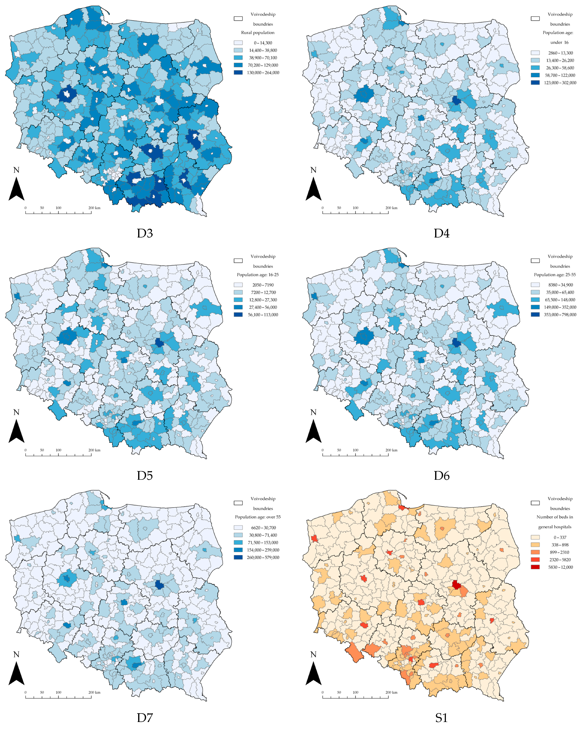
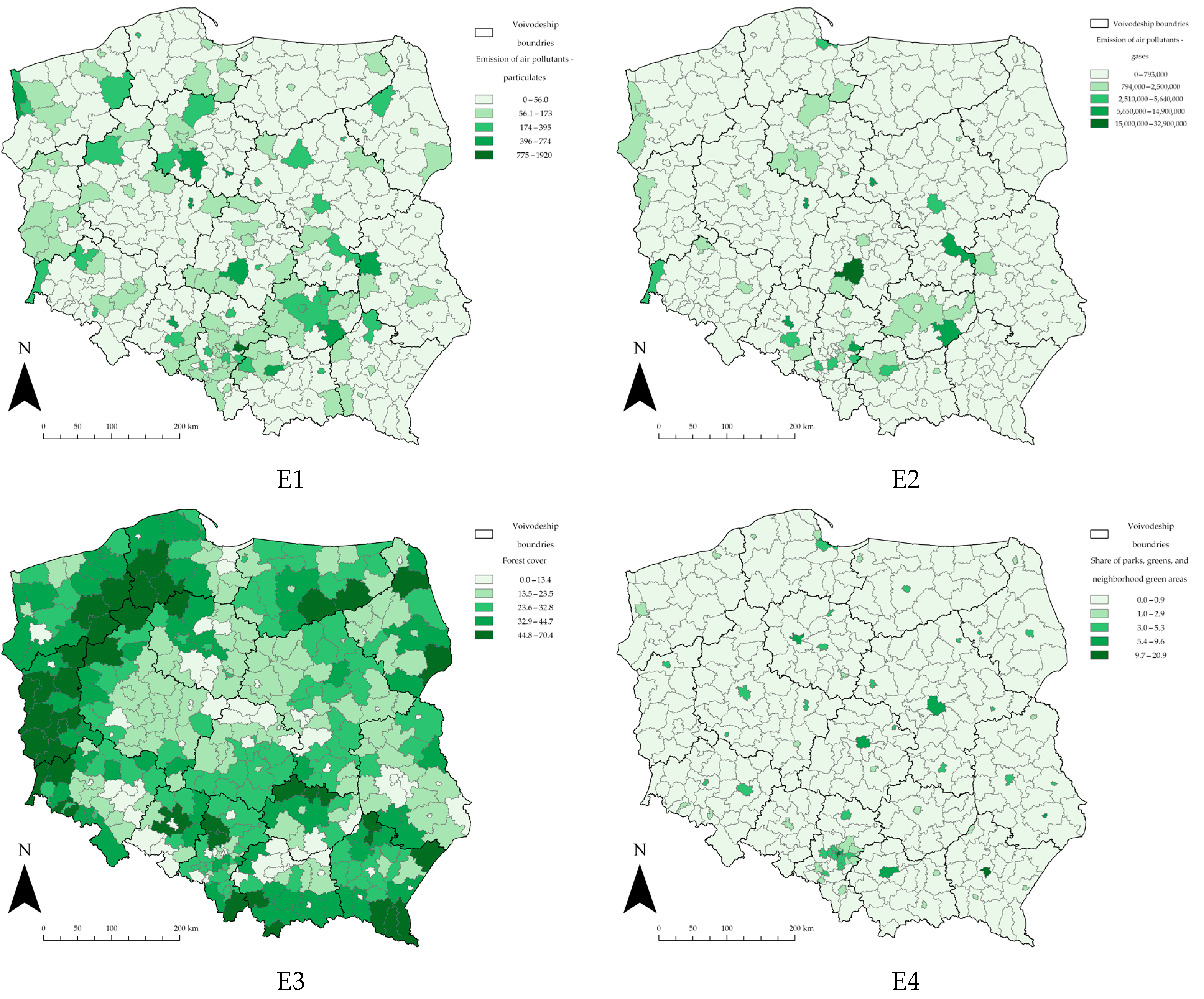
Tabular data containing the number of cases of SARS-CoV-2 in the counties of Poland and a variety of demographic, social, and environmental factors were merged and combined with the polygon data representing the administrative boundaries of the counties of Poland. The polygon data were obtained from the Polish National Register of Boundaries (NRB) [96]. The NRB is an official Polish spatial database, which forms the foundation for other spatial information systems and shares data concerning the administrative units of the country. The NRB covers the area of the whole country and contains information on the boundaries and basic attributes of the three-tier administrative division of the country (i.e., municipalities, counties, and voivodeships). Thus, the obtained geodatabase was used for further research. The following, in Figure 3, presents the spatial distribution of the used variables in the counties of Poland.

2.3. Research Method

Prior to the study, the authors decided to establish the null hypothesis—there is no statistical significance in all of the analyzed variables (in the case of this research—in the various demographic, social, and environmental factors, as well as in the number of cases of SARS-CoV-2 in the counties of Poland). The purpose of the null hypothesis is to test for statistical significance in the data and to verify that the results obtained are not the result of random chance. In order to assess the probability of the null hypothesis being true or false, a spatial autocorrelation analysis (Global Moran’s I) was carried out using the ArcGIS Pro 2.9 software (by Esri, Redlands, CA, USA). Spatial autocorrelation is the presence of systematic spatial variation in a variable; positive spatial autocorrelation is the tendency for areas or places close together to have similar values. The most common method for measuring spatial autocorrelation is to calculate the Moran’s I index [97,98,99,100,101]. The hypothesis test is as follows: if the Moran’s I = 0, there is no spatial autocorrelation; if the Moran’s I > 0, spatial autocorrelation exists, with positive and negative values indicating positive and negative autocorrelation.
Once the null hypothesis is rejected, it is possible to proceed to an examination of the influence of the selected variables on the number of cases of SARS-CoV-2 in the Polish counties using geographically weighted regression. Geographically weighted regression (GWR) is a method of analyzing spatial data based on regression, developed by adding local spatial weights [102,103,104,105,106]. GWR models considerably improve the modeling fit by capturing spatial heterogeneity, which is not factored into other regression models [101,106]. This model fully aligns with the first law of geography. The GWR model can be expressed as:
y i = β 0 ( u i , v i ) + k p β k ( u i , v i ) x i k + ε i
where
  • y i —dependent variable at location i
  • x i k —explanatory variable at location i
  • ( u i , v i ) —coordinate for location i
  • β 0 ( u i , v i ) —intercept location i
  • β k ( u i , v i ) —coefficient for explanatory variable k at location i
  • ε i —residual location i
The geographically weighted regression method has found application in studies regarding various infectious diseases: COVID-19 [107,108,109], AIDS [110], the Zika virus [111,112], tuberculosis [113], malaria [114], and others [115,116]. The GWR method can be used to estimate the effects of explanatory variables (in the case of this study, a number of social, demographic, and environmental factors) on the dependent variable (number of cases of SARS-CoV-2 in Polish counties) and also to identify the counties in which the influence of the variables differs and to explore and interpret the spatial non-stationarity. The ArcGIS Pro 2.9 software (by Esri, Redlands, CA, USA) was used to perform the GWR analysis.
In order to estimate the influence of the explanatory variables on the dependent variable, the R2 parameter was used. R2 (or R-squared) is the proportion of the dependent variable variance accounted for by the regression model; it is a measure of the goodness of fit and quantifies the performance of a local GWR model. R2 is called the coefficient of determination; its value varies from 0.0 to 1.0, and a higher value means that the explanatory variable explains the dependent variable better [99,117].
In order to evaluate whether or not the GWR model is biased by other factors, the spatial autocorrelation (global Moran’s I) tool was performed on the regression residuals. An unbiased model has residuals that are randomly scattered [106,118,119]. The explanatory variable explains the dependent variable well only after two requirements are met: a high value of the coefficient of determination (e.g., R2 > 0.8) as well as the weak or insignificant level of spatial autocorrelation in the residuals [106].

3. Results

3.1. Spatial Autocorrelation Analysis

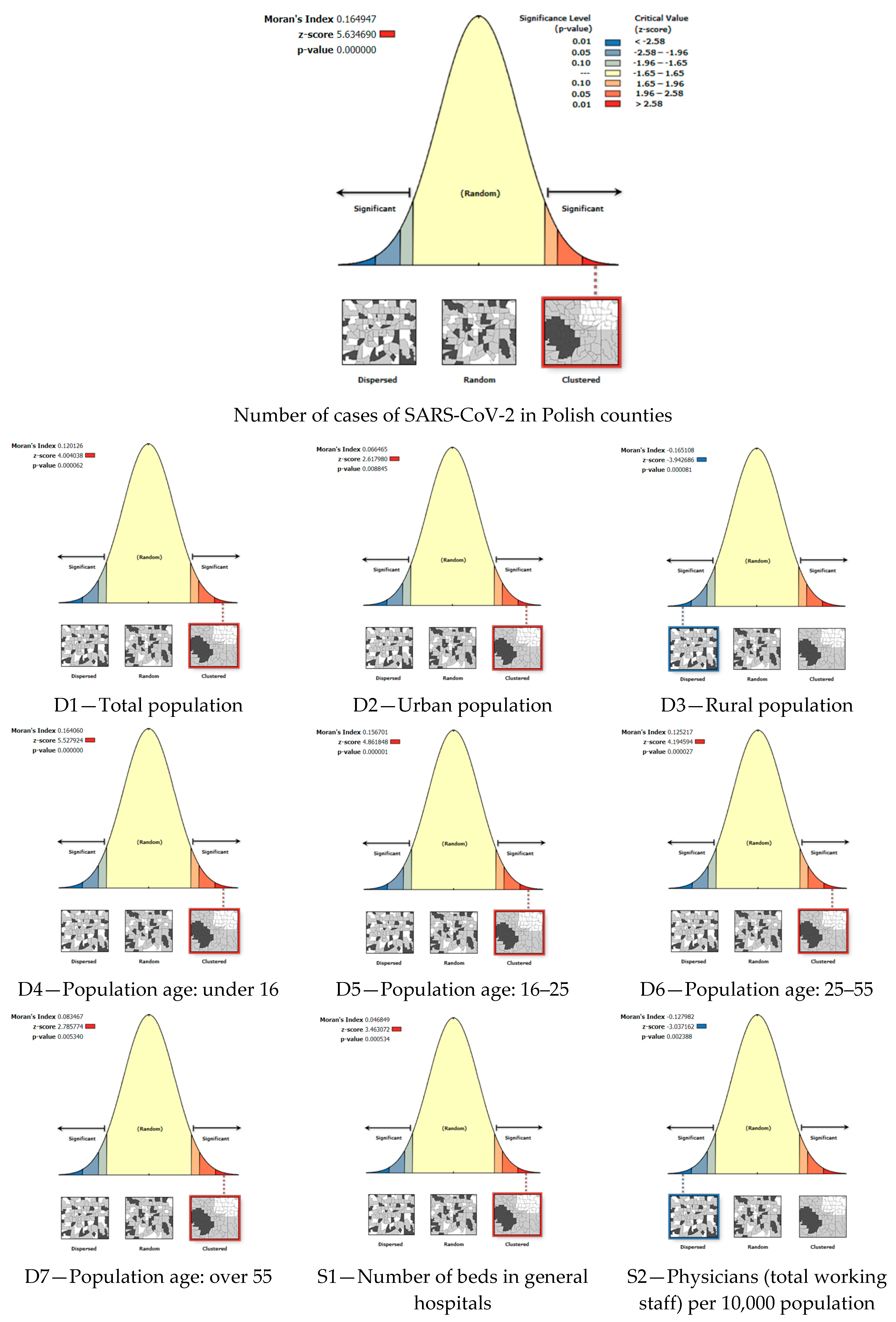
In order to evaluate the likelihood that the null hypothesis is true or false, spatial autocorrelation (global Moran’s I) analysis was performed using ArcGIS Pro 2.9 software (by Esri, Redlands, CA, USA). The spatial autocorrelation (global Moran’s I) tool measures spatial autocorrelation on the basis of feature locations and feature values; it assesses whether the expressed pattern is clustered, dispersed, or random. Below (Figure 4) are the spatial autocorrelation (global Moran’s I) reports of the analyzed variables.
A positive z-score indicates a tendency to form clusters, and it has a negative aspect—a tendency for the data to be dispersed [100,101]. The following, in Table 2, summarizes the results of the spatial autocorrelation, with the p-value, the z-score, an indication of the spatial pattern, and the confidence level for all the analyzed variables.
The obtained indicators made it possible to reject the original null hypothesis. Sixteen out of eighteen variables are statistically significant at the 0.01 confidence level, and two variables are statistically significant at the 0.05 confidence level. The positive z-scores indicate the variables that are mostly spatially clustered, and the data are characterized by spatial heterogeneity. This allows the research to continue; the next step was to assess the influence of the selected variables on the number of cases of SARS-CoV-2 in Polish counties using geographically weighted regression.

3.2. Influence of the Selected Variables on the Number of Cases of SARS-CoV-2

The analysis was performed using ArcGIS Pro 2.9 software (by Esri, Redlands, CA, USA). The polygon data representing the county boundaries in Poland were used for the study. The tabular data containing the selected variables were combined with the polygon data representing the polish counties, using the ‘Joins and Relates’ tool. Using the collected explanatory variables, the GWR analysis of the influence of the variables on the number of cases of SARS-CoV-2 in the Polish counties was carried out. The indicator values for the selected variables, as well as a statistical description of the variables, are shown in Table 3 below.
Among the analyzed variables, variable D1, the “total population,” is characterized by the highest R2 value. All variables in the “Demographic” section exhibit a very high R2 value, with the exception of variable D3 “rural population”. These results indicate that the spread of the COVID-19 pandemic took place primarily in cities; it can be closely associated with densely populated areas. The differences between the R2 values for the four age divisions (variables D4–D7) are marginal but indicate that young people (in the 16–25 age range) have a slightly smaller influence on the development of the COVID-19 pandemic in Poland.
The variables in the “Social” section also had a strong influence on the dependent variable: for variables S1, S4, S5, S6, and S7, the value was R2 > 0.80 (the highest value was obtained by the variable S7 “Benefit payments from the 500+ program”), while with variables S2 and S3 a smaller impact was observed, at R2 = 0.73 and R2 = 0.66, respectively. Variables S1–S3 determine the level of health care in the studied counties, while variables S4–S7 reflect the level of social welfare and thus identify the areas burdened by social problems resulting primarily from poverty. The areas most affected by these social problems appear to be the most susceptible to SARS-CoV-2.
The variables in the “Environmental” section did not appear to significantly influence the number of cases of SARS-CoV-2; only variable E4 has a significant R2 = 0.83.

3.3. Local R2 Estimates

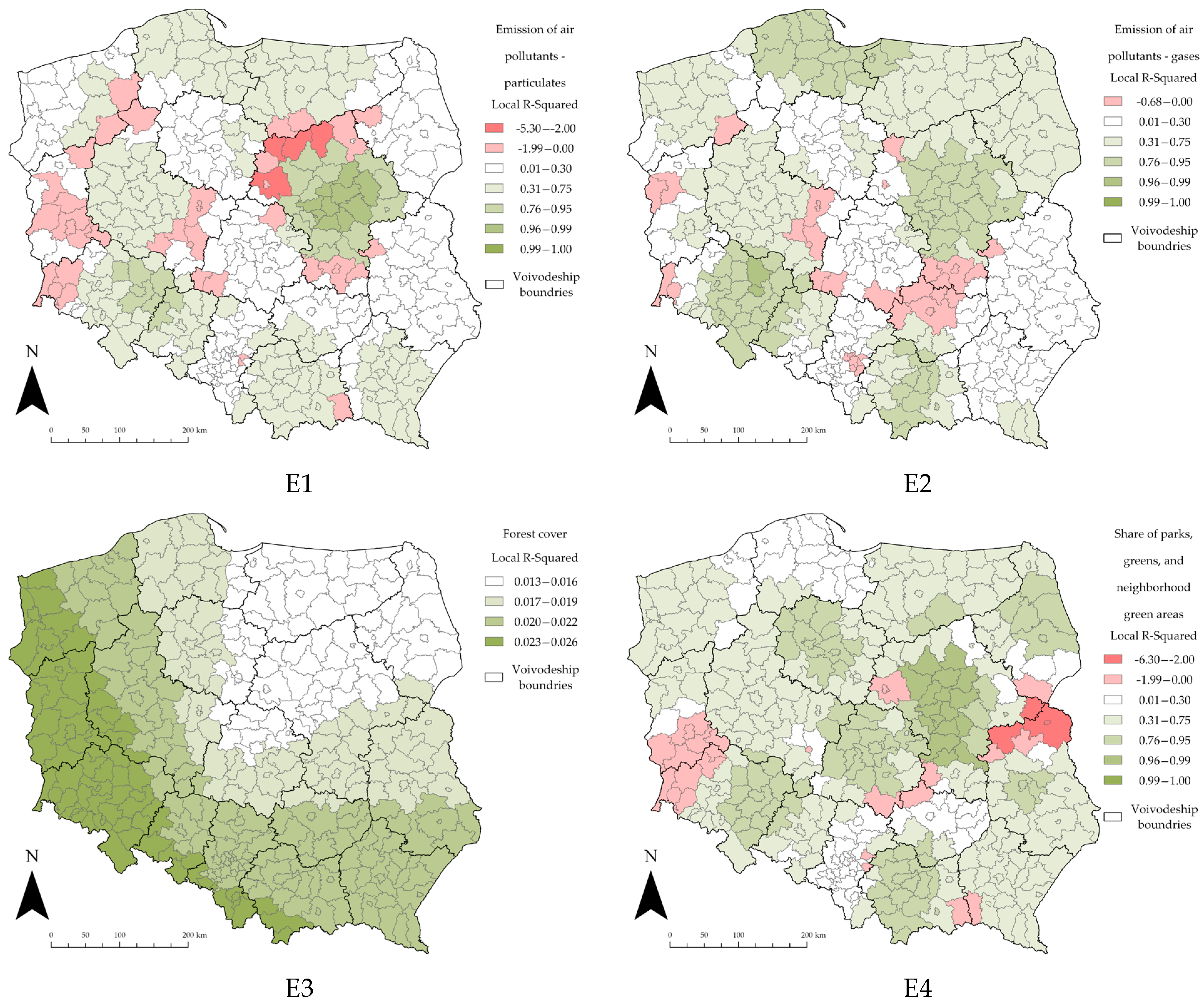
GWR allows for the exploration of spatially varying relationships. In order to estimate the spatial distribution of different variables, the local R2 estimates are presented below (Figure 5, Figure 6 and Figure 7). This is a way to visualize how the relationships between the explanatory variables and the dependent variable vary across the study area. Mapping the local R2 estimates may provide clues about important variables that may be missing from the regression model; for this study, the focus was on whether or not the number of cases of SARS-CoV-2 in Polish counties was influenced by factors other than the examined variable.
Selecting the appropriate data classification and symbolization method is an extremely important part of the cartographic process [120]. The class selection was carried out using the Jenks natural breaks method. This method is one of the most popular data classification methods [85,121,122]; it is used to reduce the variance within classes and to maximize the variance between classes. The comparison of the content of the maps is only possible if equal classification (division into classes) is used [123]. To enable the comparison of the local R2 distribution for all the explanatory variables in all three sections, the classification of the maps was standardized. This way, each class on each map corresponds to the same values; this allowed us to draw valid conclusions without any spatial-classification bias.
The boundaries of the voivodeships were overlaid on the maps; the voivodeships do not have full autonomy, but they do have some administrative independence, primarily in terms of decision making and the disposition of resources. Such a procedure allowed for additional analysis of the impact of voivodeship government actions on the progress of the COVID-19 pandemic in Poland. The following, in Figure 5, presents the local R2 values for the “Demographic” section.
The use of local R2 prediction maps revealed a significant variance in the demographic variables analyzed in the study area. The majority of the counties in the Masovian voivodeship have the highest local R2 values for all the studied variables. For the majority of variables, the counties in the southwestern part of Poland indicate a very large deviation from the R2 value for the country. By overlaying a layer of the administrative boundaries of the voivodeships, in the case of the demographic data, a significant effect of the location of the counties in a given voivodeship on the local variance of the R2 parameter can be observed (this is evident when the administrative boundary of a voivodeship overlaps with counties belonging to two different symbolization classes). Within the boundaries of a single voivodeship, the counties are often in up to two (and sometimes even one) symbolization classes.
In the case of the explanatory variable D1 (total population), the counties located in the West Pomeranian, Greater Poland, Łódź, and Masovian voivodeships appear to explain the explanatory variable the best (the local R2 values are in the fifth class, which is the highest); on the other hand, the counties located in southwestern Poland explain the explanatory variable the least effectively. The spatial distribution of the local R2 for the D2 variable almost matches that for the D1 variable. The map of the D3 variable shows an unusually large number of counties for which the local R2 values are negative or close to zero. This indicates a low level of explanation of the dependent variable, which is confirmed by the overall R2 for this explanatory variable (R2 = 0.37). Examining the age structure of the population (four variables D4–D7), it is noticeable how the results obtained are not significantly different from the results obtained for variable D1. For the D6 variable, which best explains the dependent variable (R2 = 0.99), no county is characterized with a negative local R2.
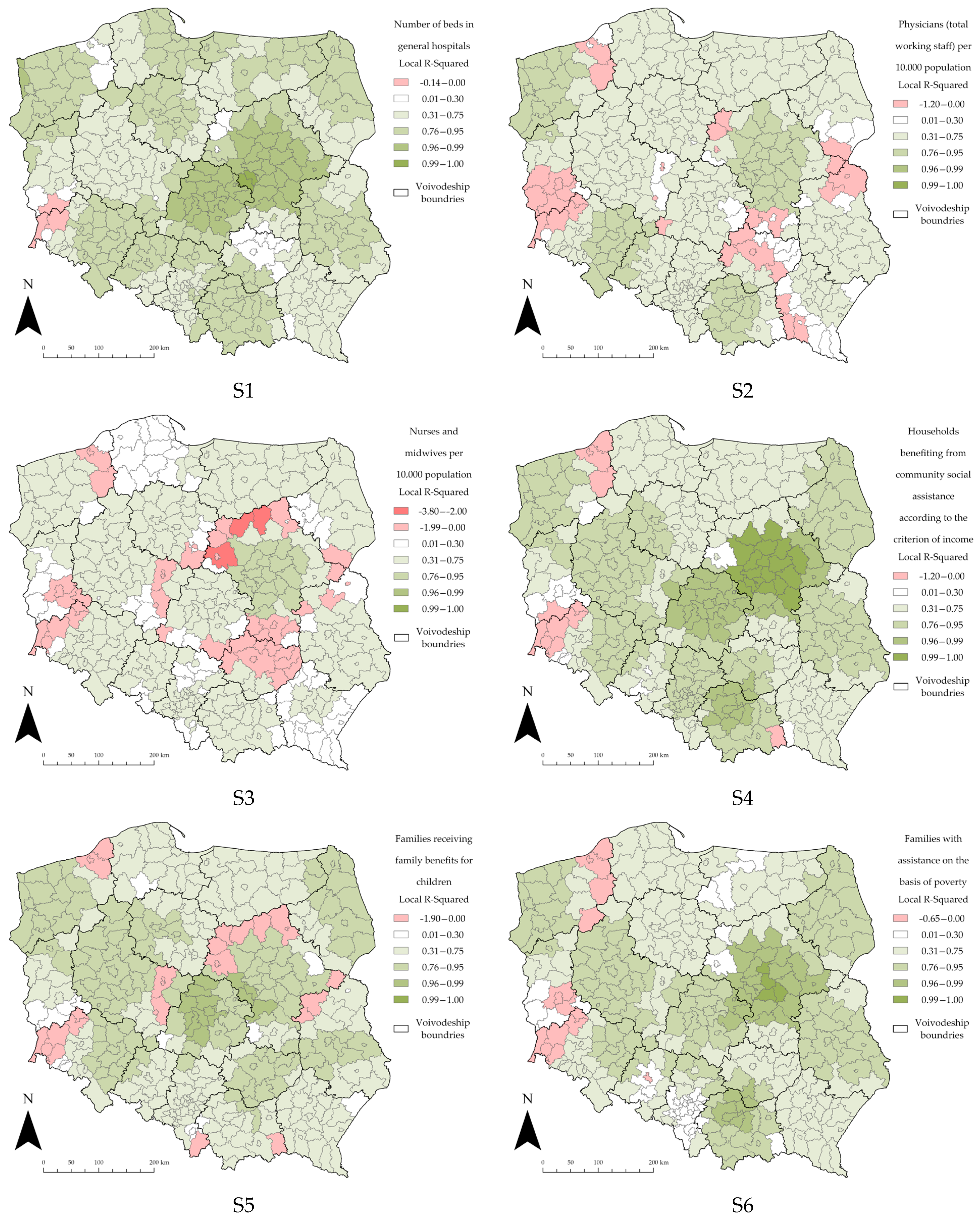
The following, in Figure 6, shows the local R2 values for the “Social” section. The bottom range of the lowest class was slightly modified to account for the decreasing local R2 value.
In the “Social” section, two thematic groups of explanatory variables can be distinguished: variables S1–S3 describe the level of healthcare and medical services, and variables S4–S7 identify the areas burdened by social problems resulting primarily from the economic exclusion of the population. For both thematic groups, the local R2 maps show far greater heterogeneity. Most of the counties in the Masovian voivodeship for almost all the explanatory variables seem to best explain the dependent variable. In addition, again the regions of southwestern Poland and the eastern counties of the West Pomeranian voivodeship explain the dependent variable the least.
In the case of the first thematic group, one can see the preservation of spatial relationships between the local R2 values. The areas indicating a lower value of local R2 appear to be almost the same across all three maps. It is most noticeable in the following areas: the eastern part of the West Pomeranian voivodeship and the southwestern part of the country, as well as almost all of the Holy Cross and Masovian voivodeships. The described counties might belong to different symbolization classes, but their mutual relationship is preserved. A similar pattern can also be observed in similar areas for the second thematic group, especially in the counties of the Masovian and West Pomeranian voivodeships.
As in the case of the “Demographic” section, one can see a large impact of the location of the counties in a given voivodeship on the local variance of the R2 parameter. For instance, this is clearly seen in the case of explanatory variables S6 and S7.
The following, in Figure 7, illustrates the local R2 values for the variables in the “Environmental” section. The bottom range of the lowest class was again slightly modified to account for the further decreasing local R2 value.
The maps of the local R2 of the “Environmental” section demonstrate the highest heterogeneity overall by far, higher than the other two sections. In addition, compared to the other sections, more counties show negative local R2 values. The highest local R2 values were again obtained in the counties of the Masovian voivodeship. Negative values of local R2 appear throughout the country but again dominate in the southwestern part of the country.
The map of the local R2 of the E3 variable “forest cover” strongly deviates from the rest of the results. In this particular case, the authors were forced to use a different classification of the data since the local R2 values are in the range of 0.013–0.026. Applying the same classification as for the other local R2 maps would place the entire case study area in a single class of 0–0.3. This situation is due to the extremely low R2 value for the entire variable, which is 0.02.

3.4. Residual Spatial Autocorrelation

In order to evaluate the performance of the GWR model, the existence of residual spatial autocorrelation was analyzed. The spatial autocorrelation (global Moran’s I) test was again performed using the ArcGIS Pro 2.9 software (by Esri, Redlands, CA, USA) to measure the residual spatial autocorrelation. The results are shown in Table 4 below.
Given the z-scores, the pattern of residuals does not appear to be significantly different than the random. Only for variables D4, D6, D7, and S7 were values indicating a weak dispersed pattern recorded (z-score between −1.96 and −1.65). The results indicate the random nature of the residuals, confirming the validity of using the GWR model.

4. Discussion

In the available databases of academic articles, the influence of the COVID-19 pandemic on various aspects related to human life has been quite thoroughly analyzed. Less emphasis was put on analyzing the influence of the various socio-environmental factors on the spread of the pandemic. The results of this research expanded the relatively small knowledge on the impact of the various factors on the progress and course of the COVID-19 pandemic.
The conducted research confirmed the research hypotheses. The established goal of the research, which was to assess the influence of various demographic, social, and environmental factors on the number of cases of SARS-CoV-2, was implemented using the geographical weighted regression (GWR) method. R2 parameter values, or the coefficients of determination, were compiled; the values vary from 0.0 to 1.0, and a higher value means that the explanatory variable explains the dependent variable better. For this research, this means that the higher the R2 value for a demographic, social, or environmental variable, the better that variable explains the number of cases of SARS-CoV-2.
The highest values of the R2 parameter were obtained for the variables in the “Demographic” section; the values for most of these variables ranged from 0.97 to 0.99. This confirms that population and the associated higher amount and intensity of human contact are the most influential factors in the development of the COVID-19 pandemic. The low R2 = 0.37 result for variable D3 “rural population” also confirms this point. The rural areas are characterized by a smaller population and a greater degree of dispersion, which implies fewer person-to-person interactions. The rural areas also tend to have reduced population mobility, which may restrict the spread of the virus.
The “Social” section can be subdivided into two thematic groups: the S1–S3 variables describe the level of health care and medical services, and the S4–S7 variables identify the areas burdened by the economic exclusion of the population. The R2 parameter for the variables in the “Social” section obtains values at an average level, in the range of 0.66–0.97. This is still a high degree of explanation of the dependent variable but clearly lower than the variables in the “Demographic” section. The highest R2 value in this section was recorded for variable S1—number of beds in general hospitals. This may be related to the fact of the increased number of healthcare facilities in urban areas, where a higher number of cases of SARS-CoV-2 virus infection have occurred. Negative R2 values were obtained in the counties of southwestern Poland: Bolesławiec county, Zgorzelec county, and Żagań county. The R2 values for variables S2 and S3, although thematically linked to variable S1, are lower, at 0.73 and 0.66, respectively. Accordingly, the number of medical personnel explains the dependent variable to a lesser extent. The areas indicating a negative value of local R2 appear across all the maps. The thematic group of the variables S3–S7, indicating the areas burdened by social problems resulting primarily from the economic exclusion of the population, is characterized by a high level of the R2 parameter. This strongly implies that the poverty-burdened areas are also highly vulnerable to the development of the COVID-19 pandemic.
The lowest R2 values (in the range of 0.02 to 0.83) for the “Environmental” section variables indicate a lower degree of explanation for the SARS-CoV-2 cases. The highest R2 value in this section was registered for variable E4, i.e., the share of parks, greens, and neighborhood green areas. This is another explanatory variable that is strongly associated with urban areas, which may explain the obtained result. The variables associated with the environmental pollution issues (E1 and E2) moderately explain the number of cases of SARS-CoV-2 infection. The R2 for these variables is 0.72 and 0.70, respectively. The lowest value of the R2 parameter was recorded for variable S3, i.e., forest cover—the obtained level of R2 = 0.02 indicates a complete lack of association of this variable with the dependent variable.
Thus, the results showed that the demographic factors best explained the number of cases of SARS-CoV-2, the social factors explained it to an average degree, and the environmental factors explained it to the lowest degree.

5. Conclusions

The application of the GWR method is not common in COVID-19 pandemic studies. In addition, most the research of this type is carried out at the country level. In the research conducted in the article, the authors developed maps of local R2 at a high level of spatial detail (research at the level of Poland’s second administrative division), allowing for more detailed conclusions and the formulation of more specific guidelines for local authorities.
The GWR method allowed for the exploration of spatially varying relationships; using maps of the local R2, it was possible to visualize how the relationships between the explanatory variables and the dependent variable vary across the study area. Considering that the COVID-19 pandemic is still ongoing, and more waves are being projected, the results obtained may be useful for local authorities in developing strategies to counter the pandemic. This is especially true for counties for which the GWR method has been able to identify deviations from the results obtained for the country as a whole. These counties can be regarded as a kind of anomaly, requiring specific, non-standard measures. Such a situation can be seen, for example, in Koszalin county, and Koszalin city county, Sławno county, and Szczecinek county (in the West Pomeranian voivodeship); Gorlice county in the Lesser Poland voivodeship; Jasło county in the Subcarpathian voivodeship; and Mława county, Ostrołęka county, Ostrów county, Płock county, Płock city county, Przasnysz country, Sierpc county, and Żuromin county (in the Masovian voivodeship), as well as the southwestern part of Poland, primarily Bolesławiec county, Lubań county, Lwówek county, Zgorzelec county, and Żagań county.
Similarly, the results of the local R2 for the variables indicating areas burdened with social problems resulting primarily from the economic exclusion of the population may be helpful to local authorities. The high association of the poverty problem with the spread of the COVID-19 pandemic has been shown above. Such a situation can be seen in particular, for example, in the counties in the central Masovian voivodeship: Białobrzegi county, Ciechanów county, Garwolin county, Grodzisk county, Grójec county, Kozienice county, Legionowo county, Warsaw city county, Warsaw West county, Maków Mazowiecki county, Mińsk Mazowiecki county, Nowy Dwór Mazowiecki county, Otwock county, Piaseczno county, Płońsk county, Pruszków county, Pułtusk county, Sochaczew county, Węgrów county, Wołomin county, Wyszków county, and Żyrardów county.
In-depth analysis combining the map of the SARS-CoV-2 cases, the maps of the indicator values, and the maps of the local R2 enabled the detection of counties where the local authorities should take specific measures, targeting the further fight against the COVID-19 pandemic in Poland. As an example, the following counties can be mentioned: Biała Podlaska county (Lubusz voivodeship), Koszalin county (West Pomeranian voivodeship), Warsaw city county, Kozienice county (Masovian voivodeship).
Biala Podlaska county is characterized by a negative R2 for the S2 variable “Physicians (total working staff) per 10,000 population”; from the “Social” section, there is a very high number of SARS-CoV-2 cases, while the number of working medical staff is considerably low. The present study indicates the need to increase the medical staff in this county in order to more effectively combat the COVID-19 pandemic. A similar situation (although to a lesser extent) is present in Koszalin county (West Pomeranian voivodeship).
In the “Environmental” section, many instances are noticeable where high levels of air pollution (represented by variables E1 and E2) largely explain the high number of cases of SARS-CoV-2. This is particularly evident in the counties of Warsaw city county, or Kozienice county (Masovian voivodeship). Warsaw, as the country’s capital, is particularly exposed to air pollution. Kozienice, the capital of Kozienice county, is the location of the second largest coal-fired power station in Poland. The largest coal-fired power station in Poland is located in Bełchatow county (Łódź voivodeship), which features distinctly in the air pollution maps, but the local R2 maps do not indicate a large influence of this phenomenon on the number of SARS-CoV-2 cases in this county; this may indicate that the local authorities are working effectively in this regard.
Such a thorough analysis of the set of maps prepared in this article can become a considerably useful tool for the authorities of a particular county, which could receive an answer to the question of to what extent to take action to further combat the COVID-19 pandemic. This might allow the specifying of actions in a particular direction in order to more effectively use the resources of the county or to confirm the effectiveness of the actions already being carried out. The proposed methodology is a ready-to-use tool for county authorities in Poland, but it can also be used in any other country with the same or greater level of spatial accuracy (lower level of administrative divisions). In this respect, this is an important innovative element of the article, as most of the previous studies focused only on the national level.

Supplementary Materials

The following supporting information can be downloaded at: https://www.mdpi.com/article/10.3390/ijerph191911881/s1; The full database of factors used for this research available to download in the Supplementary Materials.

Author Contributions

Conceptualization, M.C. and K.R.; methodology, M.C. and K.R.; software, M.C.; validation, K.R.; formal analysis, K.R.; investigation, M.C. and K.R.; resources, M.C. and K.R.; data curation, M.C.; writing—original draft preparation, M.C. and K.R.; writing—review and editing, M.C.; visualization, M.C.; supervision, K.R.; project administration, K.R. All authors have read and agreed to the published version of the manuscript.

Funding

This research received no external funding.

Institutional Review Board Statement

Not applicable.

Conflicts of Interest

The authors declare no conflict of interest. The authors declare equal contributions to the article.

References

  1. Li, Q.; Guan, X.; Wu, P.; Wang, X.; Zhou, L.; Tong, Y.; Ren, R.; Leung, K.S.M.; Lau, E.H.Y.; Wong, J.Y.; et al. Early Transmission Dynamics in Wuhan, China, of Novel Coronavirus-Infected Pneumonia. N. Engl. J. Med. 2020, 382, 1199–1207. [Google Scholar] [CrossRef] [PubMed]
  2. Zhu, N.; Zhang, D.; Wang, W.; Li, X.; Yang, B.; Song, J.; Zhao, X.; Huang, B.; Shi, W.; Lu, R.; et al. A Novel Coronavirus from Patients with Pneumonia in China, 2019. N. Engl. J. Med. 2020, 382, 727–733. [Google Scholar] [CrossRef] [PubMed]
  3. Di Gennaro, F.; Pizzol, D.; Marotta, C.; Antunes, M.; Racalbuto, V.; Veronese, N.; Smith, L. Coronavirus diseases (COVID-19) current status and future perspectives: A narrative review. Int. J. Environ. Res. Public Health 2020, 17, 2690. [Google Scholar] [CrossRef] [PubMed]
  4. Wang, C.; Pan, R.; Wan, X.; Tan, Y.; Xu, L.; Ho, C.S.; Ho, R.C. Immediate psychological responses and associated factors during the initial stage of the 2019 coronavirus disease (COVID-19) epidemic among the general population in China. Int. J. Environ. Res. Public Health 2020, 17, 1729. [Google Scholar] [CrossRef] [PubMed]
  5. Linton, N.M.; Kobayashi, T.; Yang, Y.; Hayashi, K.; Akhmetzhanov, A.R.; Jung, S.M.; Yuan, B.; Kinoshita, R.; Nishiura, H. Incubation period and other epidemiological characteristics of 2019 novel coronavirus infections with right truncation: A statistical analysis of publicly available case data. J. Clin. Med. 2020, 9, 538. [Google Scholar] [CrossRef] [PubMed]
  6. Zhang, Y.; Ma, Z.F. Impact of the COVID-19 pandemic on mental health and quality of life among local residents in Liaoning Province, China: A cross-sectional study. Int. J. Environ. Res. Public Health 2020, 17, 2381. [Google Scholar] [CrossRef]
  7. Shekhar, R.; Sheikh, A.B.; Upadhyay, S.; Singh, M.; Kottewar, S.; Mir, H.; Barrett, E.; Pal, S. COVID-19 vaccine acceptance among health care workers in the united states. Vaccines 2021, 9, 119. [Google Scholar] [CrossRef] [PubMed]
  8. Zhang, Y.; Zhang, H.; Ma, X.; Di, Q. Mental health problems during the COVID-19 pandemics and the mitigation effects of exercise: A longitudinal study of college students in China. Int. J. Environ. Res. Public Health 2020, 17, 3722. [Google Scholar] [CrossRef]
  9. Marom, P.; Zalcman, B.G.; Dankner, R. Association between Self-Classification of COVID-19 Risk Levels and Adverse Lifestyle Changes among Physically Active Older Adults Following the Coronavirus Outbreak. Int. J. Environ. Res. Public Health 2022, 19, 7039. [Google Scholar] [CrossRef]
  10. Solomou, I.; Constantinidou, F. Prevalence and predictors of anxiety and depression symptoms during the COVID-19 pandemic and compliance with precautionary measures: Age and sex matter. Int. J. Environ. Res. Public Health 2020, 17, 4924. [Google Scholar] [CrossRef]
  11. Clemente-Suárez, V.J.; Navarro-Jiménez, E.; Jimenez, M.; Hormeño-Holgado, A.; Martinez-Gonzalez, M.B.; Benitez-Agudelo, J.C.; Perez-Palencia, N.; Laborde-Cárdenas, C.C.; Tornero-Aguilera, J.F. Impact of COVID-19 pandemic in public mental health: An extensive narrative review. Sustainability 2021, 13, 3221. [Google Scholar] [CrossRef]
  12. Meyer, J.; McDowell, C.; Lansing, J.; Brower, C.; Smith, L.; Tully, M.; Herring, M. Changes in physical activity and sedentary behavior in response to COVID-19 and their associations with mental health in 3052 us adults. Int. J. Environ. Res. Public Health 2020, 17, 6469. [Google Scholar] [CrossRef]
  13. Jin, Y.; Yang, H.; Ji, W.; Wu, W.; Chen, S.; Zhang, W.; Duan, G. Virology, epidemiology, pathogenesis, and control of COVID-19. Viruses 2020, 12, 372. [Google Scholar] [CrossRef] [PubMed]
  14. Lorent, D.; Nowak, R.; Roxo, C.; Lenartowicz, E.; Makarewicz, A.; Zaremba, B.; Nowak, S.; Kuszel, L.; Stefaniak, J.; Kierzek, R.; et al. Prevalence of Anti-SARS-CoV-2 Antibodies in Poznań, Poland, after the First Wave of the COVID-19 Pandemic. Vaccines 2021, 9, 541. [Google Scholar] [CrossRef] [PubMed]
  15. Sallam, M. COVID-19 vaccine hesitancy worldwide: A concise systematic review of vaccine acceptance rates. Vaccines 2021, 9, 160. [Google Scholar] [CrossRef]
  16. Sallam, M.; Dababseh, D.; Eid, H.; Al-Mahzoum, K.; Al-Haidar, A.; Taim, D.; Yaseen, A.; Ababneh, N.A.; Bakri, F.G.; Mahafzah, A. High rates of COVID-19 vaccine hesitancy and its association with conspiracy beliefs: A study in jordan and kuwait among other arab countries. Vaccines 2021, 9, 42. [Google Scholar] [CrossRef] [PubMed]
  17. Kolifarhood, G.; Aghaali, M.; Saadati, H.M.; Taherpour, N.; Rahimi, S.; Izadi, N.; Nazari, S.S.H. Epidemiological and Clinical Aspects of COVID-19: A Narrative Review. Arch. Acad. Emerg. Med. 2020, 8, e41. [Google Scholar]
  18. Hsieh, K.-Y.; Li, D.-J.; Chou, F.H.-C.; Hsu, S.-T.; Wu, H.-C.; Chou, L.-S.; Wu, P.-J.; Lin, G.-G.; Chen, W.-J.; Liu, C.-L.; et al. Relationship of Societal Adaptation with Vaccine Worries among Healthcare Workers during the COVID-19 Pandemic: The Mediating Effects of Posttraumatic Stress Disorder. Int. J. Environ. Res. Public Health 2022, 19, 9498. [Google Scholar] [CrossRef]
  19. Vellappally, S.; Naik, S.; Alsadon, O.; Al-Kheraif, A.A.; Alayadi, H.; Jaber Alsiwat, A.; Kumar, A.; Hashem, M.; Varghese, N.; George Thomas, N.; et al. Perception of COVID-19 Booster Dose Vaccine among Healthcare Workers in India and Saudi Arabia. Int. J. Environ. Res. Public Health 2022, 19, 8942. [Google Scholar] [CrossRef]
  20. Sanchez-Oliver, J.; García-Fernández, J.; Azzouzi, S.; Stratton, C.; Muñoz-Velasco, L.P.; Wang, K.; Fourtassi, M.; Hong, B.-Y.; Cooper, R.; Balikuddembe, J.K.; et al. The Impact of the COVID-19 Pandemic on Healthy Lifestyle Behaviors and Perceived Mental and Physical Health of People Living with Non-Communicable Diseases: An International Cross-Sectional Survey. Int. J. Environ. Res. Public Health 2022, 19, 8023. [Google Scholar]
  21. Kilani, H.A.; Bataineh, M.F.; Al-Nawayseh, A.; Atiyat, K.; Obeid, O.; Abu-Hilal, M.M.; Mansi, T.; Al-Kilani, M.; Al-Kitani, M.; El-Saleh, M.; et al. Healthy lifestyle behaviors are major predictors of mental wellbeing during COVID-19 pandemic confinement: A study on adult Arabs in higher educational institutions. PLoS ONE 2020, 15, e0243524. [Google Scholar] [CrossRef] [PubMed]
  22. Novita, S.; Andriani, D.; Erika; Lipowski, M.; Lipowska, M. Anxiety towards COVID-19, Fear of Negative Appearance, Healthy Lifestyle, and Their Relationship with Well-Being during the Pandemic: A Cross-Cultural Study between Indonesia and Poland. Int. J. Environ. Res. Public Health 2022, 19, 7525. [Google Scholar] [CrossRef]
  23. Bentlage, E.; Ammar, A.; How, D.; Ahmed, M.; Trabelsi, K.; Chtourou, H.; Brach, M. Practical recommendations for maintaining active lifestyle during the COVID-19 pandemic: A systematic literature review. Int. J. Environ. Res. Public Health 2020, 17, 6265. [Google Scholar] [CrossRef] [PubMed]
  24. Gualano, M.R.; Lo Moro, G.; Voglino, G.; Bert, F.; Siliquini, R. Effects of COVID-19 lockdown on mental health and sleep disturbances in Italy. Int. J. Environ. Res. Public Health 2020, 17, 4779. [Google Scholar] [CrossRef] [PubMed]
  25. Taff, B.D.; Rice, W.L.; Lawhon, B.; Newman, P. Who started, stopped, and continued participating in outdoor recreation during the COVID-19 pandemic in the united states? Results from a national panel study. Land 2021, 10, 1396. [Google Scholar] [CrossRef]
  26. Burnett, H.; Olsen, J.R.; Mitchell, R. Green Space Visits and Barriers to Visiting during the COVID-19 Pandemic: A Three-Wave Nationally Representative Cross-Sectional Study of UK Adults. Land 2022, 11, 503. [Google Scholar] [CrossRef]
  27. Huerta, C.M.; Utomo, A. Barriers Affecting Women’s Access to Urban Green Spaces during the COVID-19 Pandemic. Land 2022, 11, 560. [Google Scholar] [CrossRef]
  28. MacKinnon, M.; MacKinnon, R.; Pedersen Zari, M.; Glensor, K.; Park, T. Urgent Biophilia: Green Space Visits in Wellington, New Zealand, during the COVID-19 Lockdowns. Land 2022, 11, 793. [Google Scholar] [CrossRef]
  29. Feng, X.; Astell-Burt, T. Perceived Qualities, Visitation and Felt Benefits of Preferred Nature Spaces during the COVID-19 Pandemic in Australia: A Nationally-Representative Cross-Sectional Study of 2940 Adults. Land 2022, 11, 904. [Google Scholar] [CrossRef]
  30. Khalilnezhad, M.R.; Ugolini, F.; Massetti, L. Attitudes and behaviors toward the use of public and private green space during the COVID-19 pandemic in Iran. Land 2021, 10, 1085. [Google Scholar] [CrossRef]
  31. Grigoletto, A.; Loi, A.; Latessa, P.M.; Marini, S.; Rinaldo, N.; Gualdi-Russo, E.; Zaccagni, L.; Toselli, S. Physical Activity Behavior, Motivation and Active Commuting: Relationships with the Use of Green Spaces in Italy. Int. J. Environ. Res. Public Health 2022, 19, 9248. [Google Scholar] [CrossRef] [PubMed]
  32. Ueno, Y.; Kato, S.; Mase, T.; Funamoto, Y.; Hasegawa, K. Human Flow Dataset Reveals Changes in Citizens’ Outing Behaviors including Greenspace Visits before and during the First Wave of the COVID-19 Pandemic in Kanazawa, Japan. Int. J. Environ. Res. Public Health 2022, 19, 8728. [Google Scholar] [CrossRef]
  33. Han, S.; Bohannon, C.L.; Kwon, Y. How has the COVID-19 pandemic affected the perceptions of public space employees? Land 2021, 10, 1332. [Google Scholar] [CrossRef]
  34. Low, S.; Smart, A. Thoughts about Public Space during COVID-19 Pandemic. City Soc. 2020, 32, 1–5. [Google Scholar]
  35. Cheshmehzangi, A. 10 Adaptive Measures for Public Places to face the COVID-19 Pandemic Outbreak. City Soc. 2020, 32, 1–10. [Google Scholar]
  36. James, A.C. Don’t stand so close to me: Public spaces, behavioral geography, and COVID-19. Dialogues Hum. Geogr. 2020, 10, 187–190. [Google Scholar] [CrossRef]
  37. Lai, K.Y.; Webster, C.; Kumari, S.; Sarkar, C. The nature of cities and the COVID-19 pandemic. Curr. Opin. Environ. Sustain. 2020, 46, 27–31. [Google Scholar] [CrossRef]
  38. Bereitschaft, B.; Scheller, D. How Might the COVID-19 Pandemic Affect 21st Century Urban Design, Planning, and Development? Urban Sci. 2020, 4, 56. [Google Scholar] [CrossRef]
  39. Samuelsson, K.; Barthel, S.; Colding, J.; Macassa, G.; Giusti, M. Urban Nature as a Source of Resilience during Social Distancing Amidst the Coronavirus Pandemic; OSF Preprints: Belleville, WI, USA, 2020. [Google Scholar]
  40. Liu, L. Emerging study on the transmission of the Novel Coronavirus (COVID-19) from urban perspective: Evidence from China. Cities 2020, 103, 102759. [Google Scholar] [CrossRef]
  41. Iranmanesh, A.; Alpar Atun, R. Reading the changing dynamic of urban social distances during the COVID-19 pandemic via Twitter. Eur. Soc. 2021, 23, S872–S886. [Google Scholar] [CrossRef]
  42. Lu, H.; Xia, M.; Qin, Z.; Lu, S.; Guan, R.; Yang, Y.; Miao, C.; Chen, T. The Built Environment Assessment of Residential Areas in Wuhan during the Coronavirus Disease (COVID-19) Outbreak. Int. J. Environ. Res. Public Health 2022, 19, 7814. [Google Scholar] [CrossRef] [PubMed]
  43. Xiang, W.; Chen, L.; Peng, Q.; Wang, B.; Liu, X. How Effective Is a Traffic Control Policy in Blocking the Spread of COVID-19? A Case Study of Changsha, China. Int. J. Environ. Res. Public Health 2022, 19, 7884. [Google Scholar] [CrossRef]
  44. Park, S.-J.; Lee, K.-T.; Im, J.-B.; Kim, J.-H. The Need for Smart Architecture Caused by the Impact of COVID-19 upon Architecture and City: A Systematic Literature Review. Sustainability 2022, 14, 7900. [Google Scholar] [CrossRef]
  45. Thomson, B. The COVID-19 Pandemic: A Global Natural Experiment. Circulation 2020, 142, 14–16. [Google Scholar] [CrossRef] [PubMed] [Green Version]
  46. Koh, D. Migrant workers and COVID-19. Occup. Environ. Med. 2020, 77, 634–636. [Google Scholar] [CrossRef]
  47. Giorgi, G.; Lecca, L.I.; Alessio, F.; Finstad, G.L.; Bondanini, G.; Lulli, L.G.; Arcangeli, G.; Mucci, N. COVID-19-related mental health effects in the workplace: A narrative review. Int. J. Environ. Res. Public Health 2020, 17, 7857. [Google Scholar] [CrossRef]
  48. Yu, W.; Alipio, C.; Wan, J.; Mane, H.; Nguyen, Q.C. Social Network Analysis on the Mobility of Three Vulnerable Population Subgroups: Domestic Workers, Flight Crews, and Sailors during the COVID-19 Pandemic in Hong Kong. Int. J. Environ. Res. Public Health 2022, 19, 7565. [Google Scholar] [CrossRef]
  49. Chen, L.; Zhang, G. COVID-19 Effects on Arbitrage Trading in the Energy Market. Energies 2022, 15, 4584. [Google Scholar] [CrossRef]
  50. Ahundjanov, B.B.; Akhundjanov, S.B.; Okhunjanov, B.B. Information search and financial markets under COVID-19. Entropy 2020, 22, 791. [Google Scholar] [CrossRef]
  51. Cao, K.H.; Li, Q.; Liu, Y.; Woo, C.K. COVID-19’s adverse effects on a stock market index. Appl. Econ. Lett. 2021, 28, 1157–1161. [Google Scholar] [CrossRef]
  52. Sharif, A.; Aloui, C.; Yarovaya, L. COVID-19 pandemic, oil prices, stock market, geopolitical risk and policy uncertainty nexus in the US economy: Fresh evidence from the wavelet-based approach. Int. Rev. Financ. Anal. 2020, 70, 101496. [Google Scholar] [CrossRef]
  53. Ghiani, E.; Galici, M.; Mureddu, M.; Pilo, F. Impact on electricity consumption and market pricing of energy and ancillary services during pandemic of COVID-19 in Italy. Energies 2020, 13, 3357. [Google Scholar] [CrossRef]
  54. Navon, A.; Machlev, R.; Carmon, D.; Onile, A.E.; Belikov, J.; Levron, Y. Effects of the COVID-19 pandemic on energy systems and electric power grids—A review of the challenges ahead. Energies 2021, 14, 1056. [Google Scholar] [CrossRef]
  55. Mas-Coma, S.; Jones, M.K.; Marty, A.M. COVID-19 and globalization. One Health 2020, 9, 100132. [Google Scholar] [CrossRef] [PubMed]
  56. Liu, H.; Manzoor, A.; Wang, C.; Zhang, L.; Manzoor, Z. The COVID-19 outbreak and affected countries stock markets response. Int. J. Environ. Res. Public Health 2020, 17, 2800. [Google Scholar] [CrossRef]
  57. Chmielewska, A.; Ciski, M.; Renigier-Biłozor, M. Residential real estate investors’ motives under pandemic conditions. Cities 2022, 128, 103801. [Google Scholar] [CrossRef]
  58. Naeem, W.; Kim, J.; Lee, Y.G. Spatiotemporal Variations in the Air Pollutant NO2 in Some Regions of Pakistan, India, China, and Korea, before and after COVID-19, Based on Ozone Monitoring Instrument Data. Atmosphere 2022, 13, 986. [Google Scholar] [CrossRef]
  59. Franch-Pardo, I.; Napoletano, B.M.; Rosete-Verges, F.; Billa, L. Spatial analysis and GIS in the study of COVID-19. A review. Sci. Total Environ. 2020, 739, 140033. [Google Scholar] [CrossRef]
  60. Asfaw, H.; Karuppannan, S.; Erduno, T.; Almohamad, H.; Abdullah, A.; Dughairi, A.; Al-Mutiry, M.; Abdo, H.G. Evaluation of Vulnerability Status of the Infection Risk to COVID-19 Using Geographic Information Systems (GIS) and Multi-Criteria Decision Analysis (MCDA): A Case Study of Addis Ababa City, Ethiopia. Int. J. Environ. Res. Public Health 2022, 19, 7811. [Google Scholar] [CrossRef]
  61. Sánchez-Sánchez, J.A.; Chuc, V.M.K.; Canché, E.A.R.; Uscanga, F.J.L. Vulnerability Assessing Contagion Risk of COVID-19 Using Geographic Information Systems and Multi-Criteria Decision Analysis: Case Study Chetumal, México. In Proceedings of the 1st GIS LATAM Conference, GIS LATAM 2020, Mexico City, Mexico, 28–30 September 2020; Springer: Cham, Switzerland, 2020. [Google Scholar]
  62. Murugesan, B.; Karuppannan, S.; Mengistie, A.T.; Ranganathan, M.; Gopalakrishnan, G. Distribution and Trend Analysis of COVID-19 in India: Geospatial Approach. J. Geogr. Stud. 2020, 4, 1–9. [Google Scholar] [CrossRef]
  63. Zhou, C.; Su, F.; Pei, T.; Zhang, A.; Du, Y.; Luo, B.; Cao, Z.; Wang, J.; Yuan, W.; Zhu, Y.; et al. COVID-19: Challenges to GIS with Big Data. Geogr. Sustain. 2020, 1, 77–87. [Google Scholar] [CrossRef]
  64. Pourghasemi, H.R.; Pouyan, S.; Farajzadeh, Z.; Sadhasivam, N.; Heidari, B.; Babaei, S.; Tiefenbacher, J.P. Assessment of the outbreak risk, mapping and infection behavior of COVID-19: Application of the autoregressive integrated-moving average (ARIMA) and polynomial models. PLoS ONE 2020, 15, e0236238. [Google Scholar] [CrossRef] [PubMed]
  65. Kamel Boulos, M.N.; Geraghty, E.M. Geographical tracking and mapping of coronavirus disease COVID-19/severe acute respiratory syndrome coronavirus 2 (SARS-CoV-2) epidemic and associated events around the world: How 21st century GIS technologies are supporting the global fight against outbr. Int. J. Health Geogr. 2020, 19, 8. [Google Scholar] [CrossRef]
  66. Lokhande, T.; Yang, X.; Xie, Y.; Cook, K.; Liang, J.; LaBelle, S.; Meyers, C. GIS-based classroom management system to support COVID-19 social distance planning. Comput. Urban Sci. 2022, 2, 11. [Google Scholar] [CrossRef]
  67. Hu, M.; Roberts, J.D.; Azevedo, G.P.; Milner, D. The role of built and social environmental factors in COVID-19 transmission: A look at America’s capital city. Sustain. Cities Soc. 2021, 65, 102580. [Google Scholar] [CrossRef]
  68. Md Iderus, N.H.; Lakha Singh, S.S.; Mohd Ghazali, S.; Yoon Ling, C.; Cia Vei, T.; Md Zamri, A.S.S.; Ahmad Jaafar, N.; Ruslan, Q.; Ahmad Jaghfar, N.H.; Gill, B.S. Correlation between Population Density and COVID-19 Cases during the Third Wave in Malaysia: Effect of the Delta Variant. Int. J. Environ. Res. Public Health 2022, 19, 7439. [Google Scholar] [CrossRef]
  69. Ma, Y.; Zhao, Y.; Liu, J.; He, X.; Wang, B.; Fu, S.; Yan, J.; Niu, J.; Zhou, J.; Luo, B. Effects of temperature variation and humidity on the death of COVID-19 in Wuhan, China. Sci. Total Environ. 2020, 724, 138226. [Google Scholar] [CrossRef] [PubMed]
  70. Xie, J.; Zhu, Y. Association between ambient temperature and COVID-19 infection in 122 cities from China. Sci. Total Environ. 2020, 724, 138201. [Google Scholar] [CrossRef]
  71. Ciski, M.; Rzasa, K. Cultural Parks in the Spatial Planning System in Poland. In Proceedings of the 2018 Baltic Geodetic Congress (BGC Geomatics), Olsztyn, Poland, 21–23 June 2017; IEEE: Piscataway, NJ, USA, 2018; pp. 145–149. [Google Scholar]
  72. Ciski, M.; Rząsa, K. Threats to Cultural Heritage Caused by the Global Sea Level Rise as a Result of the Global Warming. Water 2021, 13, 2577. [Google Scholar] [CrossRef]
  73. Szarek-Iwaniuk, P.; Dawidowicz, A.; Senetra, A. Methodology for Precision Land Use Mapping towards Sustainable Urbanized Land Development. J. Environ. Res. Public Health 2022, 19, 3633. [Google Scholar] [CrossRef] [PubMed]
  74. Devkota, M.; Hatfield, G.; Chintala, R. Effect of Sample Size on the Performance of Ordinary Least Squares and Geographically Weighted Regression. Br. J. Math. Comput. Sci. 2014, 4, 1–21. [Google Scholar] [CrossRef]
  75. Michał Rogalski (@micalrg)/Twitter. Available online: https://twitter.com/micalrg (accessed on 6 July 2022).
  76. Rogalski, M. Dane o COVID-19 Według Powiatów. Available online: https://bit.ly/covid19_powiaty (accessed on 6 July 2022).
  77. Rogalski, M. Archiwum Danych Powiatowych Raportowanych Przez Ministerstwo Zdrowia. Available online: https://bit.ly/covid19_archiwumMZ (accessed on 6 July 2022).
  78. Kaczmarek, T.; Mikuła, Ł. Presidential Elections in Poland During the COVID-19 Pandemic: An Unexpected Challenge for Political Actors and the Relationship Between Central Government and Local Government. In Local Government and the COVID-19 Pandemic; Springer: Cham, Switzerland, 2022; pp. 451–479. [Google Scholar]
  79. Lipowicz, I.; Szpor, G. Neue Aspekte der Desinformation. Datenschutz Datensicherh. -DuD 2021, 45, 381–384. [Google Scholar] [CrossRef]
  80. Kowalski, P.A.; Szwagrzyk, M.; Kielpinska, J.; Konior, A.; Kusy, M. Numerical analysis of factors, pace and intensity of the corona virus (COVID-19) epidemic in Poland. Ecol. Inform. 2021, 63, 101284. [Google Scholar] [CrossRef] [PubMed]
  81. Parysek, J.J.; Mierzejewska, L. Cities in the epidemic, the epidemic in cities: Reconstruction of COVID-19 development in Polish cities. Cities 2022, 125, 103676. [Google Scholar] [CrossRef] [PubMed]
  82. Sawik, B.; Płonka, J. Project and Prototype of Mobile Application for Monitoring the Global COVID-19 Epidemiological Situation. Int. J. Environ. Res. Public Health 2022, 19, 1416. [Google Scholar] [CrossRef]
  83. Śleszyński, P. Prawidłowości Przebiegu dyfuzji Przestrzennej rejestrowanych zakażeń koronawirusem SARS-CoV-2 w Polsce w Pierwszych 100 dniach ePidemii. Czas. Geogr. 2020; in press. [Google Scholar]
  84. Duszyński, J.; Afelt, A.; Ochab-Marcinek, A.; Owczuk, R.; Pyrć, K.; Rosińska, M.; Rychard, A.; Smiatacz, T. Zrozumieć COVID-19 Opracowanie Zespołu ds. COVID-19 przy Prezesie Polskiej Akademii Nauk; Polska Akademia Nauk: Warsaw, Poland, 2020. [Google Scholar]
  85. Rzasa, K.; Ciski, M. Determination of the level of sustainable development of the cities—A proposal for a method of classifying objects based on natural breaks. Acta Sci. Pol. Adm. Locorum 2021, 20, 215–239. [Google Scholar] [CrossRef]
  86. Lenart-Bugla, M.; Łuc, M.; Pawłowski, M.; Szcześniak, D.; Seifert, I.; Wiegelmann, H.; Gerhardus, A.; Wolf-Ostermann, K.; Rouwette, E.A.J.A.; Ikram, M.A.; et al. What Do We Know about Social and Non-Social Factors Influencing the Pathway from Cognitive Health to Dementia? A Systematic Review of Reviews. Brain Sci. 2022, 12, 1214. [Google Scholar] [CrossRef]
  87. Karmowska, G. Zróżnicowanie rozwoju powiatów województwa zachodniopomorskiego. Pr. Nauk. Uniw. Ekon. Wroc. 2013, 307, 233–246. [Google Scholar]
  88. Józefowicz, K.; Smolińska, K. Poziom rozwoju społeczno-gospodarczego w powiatach województwa wielkopolskiego. J. Tour. Reg. Dev. 2019, 11, 37–49. [Google Scholar] [CrossRef]
  89. Miłek, D. Zróżnicowanie rozwoju społeczno-gospodarczego powiatów województwa świętokrzyskiego. Wiad. Stat. 2018, 6, 39–56. [Google Scholar]
  90. Sompolska-Rzechuła, A. Zróżnicowanie rozwoju społecznego w ujęciu przestrzennym. Wiad. Stat. Pol. Stat. 2016, 1, 62–78. [Google Scholar]
  91. Bożek, J.; Szewczyk, J. Evaluation of the level of social development of poviats in Małopolskie Voivodship with the use of a dynamic synthetic measure. Wiad. Stat. Pol. Stat. 2021, 66, 45–63. [Google Scholar] [CrossRef]
  92. Siudek, T.; Drabarczyk, K.; Zawojska, A. Rozwój społeczny powiatów województwa mazowieckiego—Kwantyfikacja i ocena. Zesz. Nauk. SGGW Ekon. Organ. Gospod. Żywnościowej 2019, 123, 17–42. [Google Scholar] [CrossRef]
  93. Sun, B.; Wang, H.; Ortiz, J.; Huang, J.; Zhao, C. A Decomposed Data Analysis Approach to Assessing City Sustainable Development Performance: A Network DEA Model with a Slack-Based Measure. Sustainability 2022, 14, 11037. [Google Scholar] [CrossRef]
  94. Kim, S.Y.; Kim, B.H.S. The Effect of Urban Green Infrastructure on Disaster Mitigation in Korea. Sustainability 2017, 9, 1026. [Google Scholar] [CrossRef]
  95. Wang, Q.; Dai, H.N.; Wang, H. A smart MCDM framework to evaluate the impact of air pollution on city sustainability: A case study from China. Sustainability 2017, 9, 911. [Google Scholar] [CrossRef]
  96. Polish National Register of Borders. Available online: https://www.geoportal.gov.pl/dane/panstwowy-rejestr-granic (accessed on 11 July 2022).
  97. Tiefelsdorf, M. The saddlepoint approximation of Moran’s I’s and local Moran’s Ii’s reference distributions and their numerical evaluation. Geogr. Anal. 2002, 34, 187–206. [Google Scholar] [CrossRef]
  98. Han, F.; Sui, F. Effect of Global Moran’s I and space-time permutation scanning method in shanghai metro traffic based on ecological transportation system. Ekoloji 2019, 28, 4295–4303. [Google Scholar]
  99. Lichstein, J.W.; Simons, T.R.; Shriner, S.A.; Franzreb, K.E. Spatial autocorrelation and autoregressive models in ecology. Ecol. Monogr. 2002, 72, 445–463. [Google Scholar] [CrossRef]
  100. Mohammad Sham, N.; Anual, Z.F.; Shaharudin, R. GIS based interpolation method to urinary metal concentrations in Malaysia. Food Chem. Toxicol. 2022, 163, 112949. [Google Scholar] [CrossRef]
  101. Gao, Y.; Zhao, J.; Han, L. Exploring the spatial heterogeneity of urban heat island effect and its relationship to block morphology with the geographically weighted regression model. Sustain. Cities Soc. 2022, 76, 103431. [Google Scholar] [CrossRef]
  102. Permai, S.D.; Christina, A.; Santoso Gunawan, A.A. Fiscal decentralization analysis that affect economic performance using geographically weighted regression (GWR). Procedia Comput. Sci. 2021, 179, 399–406. [Google Scholar] [CrossRef]
  103. Mennis, J. Mapping the results of geographically weighted regression. Cartogr. J. 2006, 43, 171–179. [Google Scholar] [CrossRef]
  104. Stiller, D.; Ottinger, M.; Leinenkugel, P.; Stiller, D.; Ottinger, M.; Leinenkugel, P. Spatio-Temporal Patterns of Coastal Aquaculture Derived from Sentinel-1 Time Series Data and the Full Landsat Archive. Remote Sens. 2019, 11, 1707. [Google Scholar] [CrossRef]
  105. Brunsdon, C.; Fotheringham, A.S.; Charlton, M.E. Geographically weighted regression: A method for exploring spatial nonstationarity. Geogr. Anal. 1996, 28, 281–298. [Google Scholar] [CrossRef]
  106. Comber, A.; Brunsdon, C.; Charlton, M.; Dong, G.; Harris, R.; Lu, B.; Yihe, L.; Murakami, D.; Nakaya, T.; Wang, Y.; et al. A Route Map for Successful Applications of Geographically Weighted Regression. Geogr. Anal. 2022. [Google Scholar] [CrossRef]
  107. Ganasegeran, K.; Jamil, M.F.A.; Appannan, M.R.; Ch’ng, A.S.H.; Looi, I.; Peariasamy, K.M. Spatial Dynamics and Multiscale Regression Modelling of Population Level Indicators for COVID-19 Spread in Malaysia. Int. J. Environ. Res. Public Health 2022, 19, 2082. [Google Scholar] [CrossRef]
  108. Lyu, T.; Hair, N.; Yell, N.; Li, Z.; Qiao, S.; Liang, C.; Li, X. Temporal Geospatial Analysis of COVID-19 Pre-Infection Determinants of Risk in South Carolina. Int. J. Environ. Res. Public Health 2021, 18, 9673. [Google Scholar] [CrossRef]
  109. Zhang, J.; Wu, X.; Chow, T.E. Space-Time Cluster’s Detection and Geographical Weighted Regression Analysis of COVID-19 Mortality on Texas Counties. Int. J. Environ. Res. Public Health 2021, 18, 5541. [Google Scholar] [CrossRef]
  110. Wang, Y.; Zhao, C.; Liu, Z.; Gao, D. Spatiotemporal Analysis of AIDS Incidence and Its Influencing Factors on the Chinese Mainland, 2005–2017. Int. J. Environ. Res. Public Health 2005, 18, 1043. [Google Scholar] [CrossRef]
  111. Li, J.; Jia, K.; Liu, Y.; Yuan, B.; Xia, M.; Zhao, W. Spatiotemporal Distribution of Zika Virus and Its Spatially Heterogeneous Relationship with the Environment. Public Health 2021, 18, 290. [Google Scholar] [CrossRef]
  112. Dos Anjos, R.S.; Nóbrega, R.S.; Ferreira, H.D.S.; de Lacerda, A.P.; de Sousa-Neves, N. Exploring local and global regression models to estimate the spatial variability of Zika and Chikungunya cases in Recife, Brazil. Rev. Soc. Bras. Med. Trop. 2020, 53, 1–9. [Google Scholar] [CrossRef]
  113. Sun, W.; Gong, J.; Zhou, J.; Zhao, Y.; Tan, J.; Ibrahim, A.N.; Zhou, Y. A Spatial, Social and Environmental Study of Tuberculosis in China Using Statistical and GIS Technology. Int. J. Environ. Res. Public Health 2015, 12, 1425–1448. [Google Scholar] [CrossRef]
  114. Moise, I.K.; Roy, S.S.; Nkengurutse, D.; Ndikubagenzi, J. Seasonal and Geographic Variation of Pediatric Malaria in Burundi: 2011 to 2012. Int. J. Environ. Res. Public Health 2016, 13, 425. [Google Scholar] [CrossRef]
  115. Li, S.; Ren, H.; Hu, W.; Lu, L.; Xu, X.; Zhuang, D.; Liu, Q. Spatiotemporal Heterogeneity Analysis of Hemorrhagic Fever with Renal Syndrome in China Using Geographically Weighted Regression Models. Int. J. Environ. Res. Public Health 2014, 11, 12129–12147. [Google Scholar] [CrossRef]
  116. Atique, S.; Chan, T.C.; Chen, C.C.; Hsu, C.Y.; Iqtidar, S.; Louis, V.R.; Shabbir, S.A.; Chuang, T.W. Investigating spatio-temporal distribution and diffusion patterns of the dengue outbreak in Swat, Pakistan. J. Infect. Public Health 2018, 11, 550–557. [Google Scholar] [CrossRef]
  117. Xiu, Y.; Wang, N.; Peng, F.; Wang, Q. Spatial-Temporal Variations of Water Ecosystem Services Value and Its Influencing Factors: A Case in Typical Regions of the Central Loess Plateau. Sustainability 2022, 14, 7169. [Google Scholar] [CrossRef]
  118. Yu, S.; Ye, Q.; Zhao, Q.; Li, Z.; Zhang, M.; Zhu, H.; Zhao, Z. Effects of Driving Factors on Forest Aboveground Biomass (AGB) in China’s Loess Plateau by Using Spatial Regression Models. Remote Sens. 2022, 14, 2842. [Google Scholar] [CrossRef]
  119. Yue, H.; Duan, L.; Lu, M.; Huang, H.; Zhang, X.; Liu, H. Modeling the Determinants of PM2.5 in China Considering the Localized Spatiotemporal Effects: A Multiscale Geographically Weighted Regression Method. Atmosphere 2022, 13, 627. [Google Scholar] [CrossRef]
  120. Ogryzek, M.; Ciski, M. Cartographic Methods of Presentation the Average Transaction Prices of the Undeveloped Land. Civ. Environ. Eng. Rep. 2018, 28, 85–100. [Google Scholar] [CrossRef]
  121. Khamis, N.; Sin, T.C.; Hock, G.C. Segmentation of Residential Customer Load Profile in Peninsular Malaysia using Jenks Natural Breaks. In Proceedings of the 2018 IEEE 7th International Conference on Power and Energy, PECon 2018, Kuala Lumpur, Malaysia, 3–4 December 2018; Institute of Electrical and Electronics Engineers Inc.: Piscataway, NJ, USA, 2018; pp. 128–131. [Google Scholar]
  122. Chen, J.; Yang, S.; Li, H.; Zhang, B.; Lv, J. Research on geographical environment unit division based on the method of natural breaks (Jenks). International Archives of the Photogrammetry, Remote Sensing and Spatial Information Sciences—ISPRS Archives. In Proceedings of the ISPRS/IGU/ICA Joint Workshop on Borderlands Modelling and Understanding for Global Sustainability 2013, Beijing, China, 5–6 December 2013; Volume 40, pp. 47–50. [Google Scholar]
  123. Ciski, M.; Rzasa, K.; Ogryzek, M. Use of GIS tools in sustainable heritage management—The importance of data generalization in spatial modeling. Sustainability 2019, 11, 5616. [Google Scholar] [CrossRef] [Green Version]
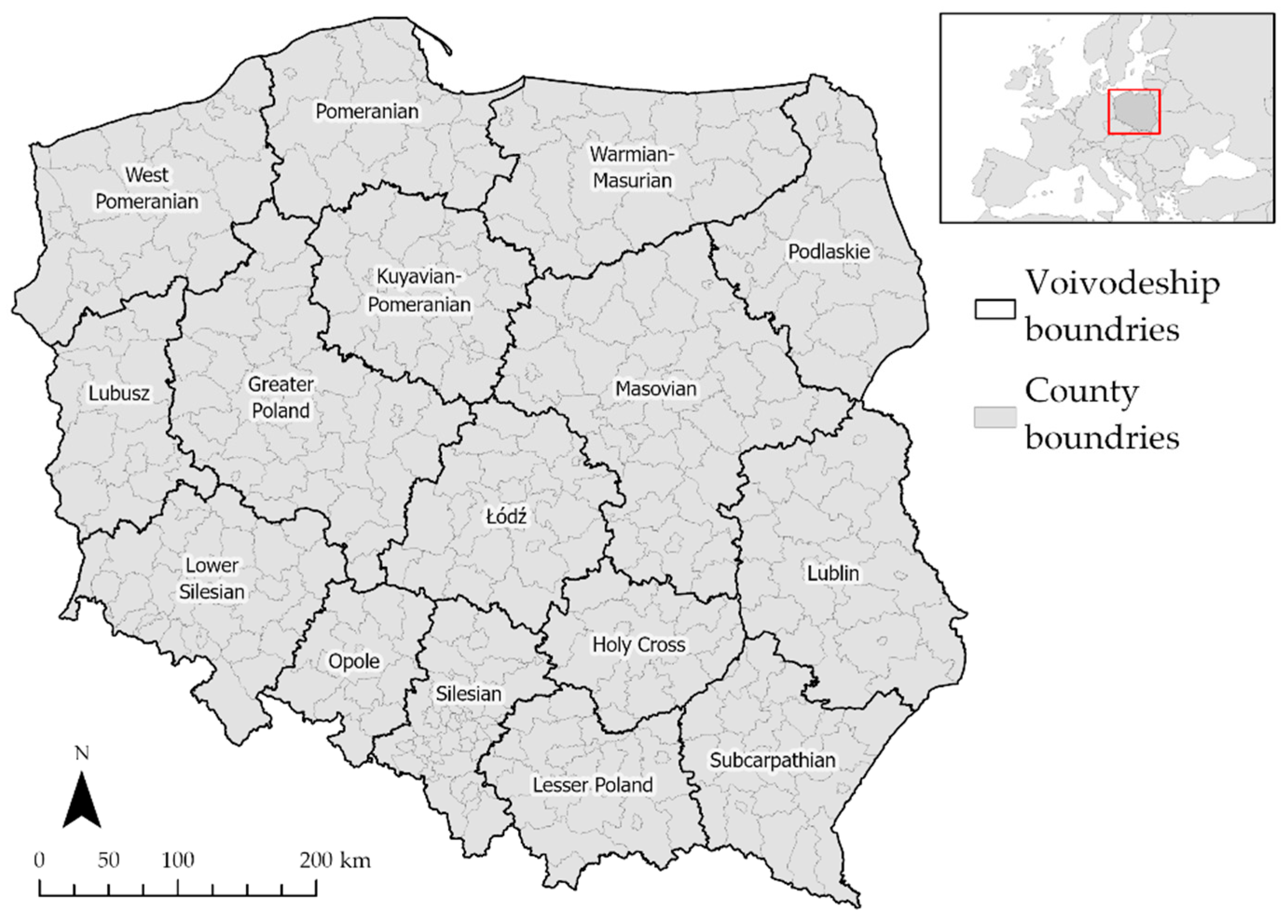
Figure 1. Study area. Source: own elaboration using ArcGIS Pro 2.9 by Esri.
Ijerph 19 11881 g001
Figure 2. Summary of confirmed cases of SARS-CoV-2 in Polish counties. Source: own elaboration using ArcGIS Pro 2.9 by Esri.
Ijerph 19 11881 g002
Figure 3. Spatial distribution of the explanatory variables in counties of Poland. Source: own elaboration using ArcGIS Pro 2.9 by Esri.
Ijerph 19 11881 g003aIjerph 19 11881 g003bIjerph 19 11881 g003cIjerph 19 11881 g003d
Figure 4. Spatial autocorrelation reports. Source: own elaboration using ArcGIS Pro 2.9 by Esri.
Ijerph 19 11881 g004aIjerph 19 11881 g004b
Figure 5. Local R2 estimates for the “Demographic” section. Source: own elaboration using ArcGIS Pro 2.9 by Esri.
Ijerph 19 11881 g005aIjerph 19 11881 g005b
Figure 6. Local R2 estimates for the “Social” section. Source: own elaboration using ArcGIS Pro 2.9 by Esri.
Ijerph 19 11881 g006aIjerph 19 11881 g006b
Figure 7. Local R2 estimates for the “Environmental” section. Source: own elaboration using ArcGIS Pro 2.9 by Esri.
Ijerph 19 11881 g007
Table 1. Selected demographic, social, and environmental factors. Source: own elaboration on the basis of data from Statistics Poland.
SectionFactor (Variable)Symbol
DemographicTotal populationD1
Urban populationD2
Rural populationD3
Population age: under 16D4
Population age: 16–25D5
Population age: 25–55D6
Population age: over 55D7
SocialNumber of beds in general hospitalsS1
Physicians (total working staff) per 10,000 populationS2
Nurses and midwives per 10,000 populationS3
Households benefiting from community social assistance according to the criterion of incomeS4
Families receiving family benefits for childrenS5
Families with assistance on the basis of povertyS6
Benefit payments from the 500+ programS7
EnvironmentalEmission of air pollutants—particulatesE1
Emission of air pollutants—gasesE2
Forest coverE3
Share of parks, greens, and neighborhood green areasE4
Table 2. Summary of the spatial autocorrelation. Source: own elaboration on the basis of ArcGIS Pro 2.9 by Esri.
Variable TypeVariablep-ValueZ-ScoreSpatial PatternConfidence Level
DependentCOVID-19 cases0.005.63Clustered1%
ExplanatoryD1—Total population0.004.00Clustered1%
D2—Urban population0.012.62Clustered1%
D3—Rural population0.00−3.94Dispersed1%
D4—Population age: under 160.005.53Clustered1%
D5—Population age: 16–250.004.86Clustered1%
D6—Population age: 25–550.004.19Clustered1%
D7—Population age: over 550.012.79Clustered1%
S1—Number of beds in general hospitals0.003.46Clustered1%
S2—Physicians (total working staff) per 10,000 population0.00−3.04Dispersed1%
S3—Nurses and midwives per
10,000 population
0.00−4.67Dispersed1%
S4—Households benefiting from community social assistance according to the criterion of income0.002.95Clustered1%
S5—Families receiving family benefits for children0.006.30Clustered1%
S6—Families with assistance on the basis of poverty0.003.29Clustered1%
S7—Benefit payments from the 500+ program0.006.24Clustered1%
E1—Emission of air pollutants—particulates0.022.41Clustered5%
E2—Emission of air pollutants—gases0.032.24Clustered5%
E3—Forest cover0.0010.41Clustered1%
E4—Share of parks, greens,
and neighborhood green areas
0.003.96Clustered1%
Table 3. R2 and statistical description of the variables. Source: own elaboration on the basis of ArcGIS Pro 2.9 by Esri.
VariableR2MeanMinMaxSTD
D1—Total population0.99 **101,006.819,914.01,790,658.0119,730.5
D2—Urban population0.95 **60,613.30.01,790,658.0122,692.5
D3—Rural population0.37 **40,393.40.0264,014.035,060.6
D4—Population age: under 160.98 **16,433.62855.0301,697.019,744.3
D5—Population age: 16–250.97 **9143.92054.0112,725.08220.1
D6—Population age: 25–550.99 **43,570.88382.0797,514.053,035.6
D7—Population age: over 550.98 **31,858.46623.0578,722.039,298.0
S1—Number of beds in general hospitals0.91 **439.00.011,970.0907.7
S2—Physicians (total working staff)
per 10,000 population
0.73 **41.12.0204.930.4
S3—Nurses and midwives
per 10,000 population
0.66 **60.62.4237.437.5
S4—Households benefiting from community social assistance according
to the criterion of income
0.94 **2171.1472.020,186.01698.4
S5—Families receiving family benefits
for children
0.86 **2653.0352.014,260.01739.9
S6—Families with assistance on the basis
of poverty
0.91 **1139.2145.010,765.0885.6
S7—Benefit payments
from the 500+ program
0.97 **80,276,961.115,183,262.01,366,004,134.090,144,295.6
E1—Emission of air pollutants—particulates0.72 *71.30.01924.0143.3
E2—Emission of air pollutants—gases0.70 *522,212.50.032,882,772.02,138,844.5
E3—Forest cover0.02 **26.00.070.413.4
E4—Share of parks, greens,
and neighborhood green areas
0.83 **0.80.020.91.9
Note: **—statistically significant at the p < 0.01 level; *—statistically significant at the p < 0.05 level.
Table 4. Spatial autocorrelation results for GWR residuals. Source: own elaboration on the basis of ArcGIS Pro 2.9 by Esri.
VariableD1D2D3D4D5D6D7S1S2S3S4S5S6S7E1E2E3E4
Residual z-score−1.26−1.280.66−1.95−1.44−1.82−1.93−1.461.35−0.81−0.340.731.33−1.70.750.330.380.01
Spatial
pattern
RRRwDRwDwDRRRRRRwDRRRR
Note: R—random; wD—weak dispersed.
Publisher’s Note: MDPI stays neutral with regard to jurisdictional claims in published maps and institutional affiliations.