
Analysis of Car-Following Behaviors under Different Conditions on the Entrance Section of Cross-River and Cross-Sea Tunnels: A Case Study of Shanghai Yangtze River Tunnel


Abstract
:1. Introduction
2. Methods
2.1. Apparatus
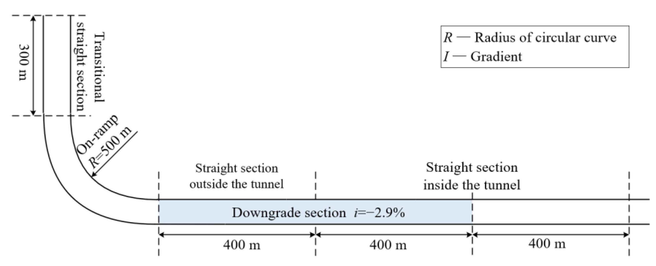
2.2. Scenarios
2.3. Data Collection Procedure
- (1)
- The experiment with different weather and traffic conditions
- (2)
- The experiment with different longitudinal slopes
2.4. Participants
2.5. Car-Following Behavior Variable
- (1)
- Distance headway
- (2)
- Time headway
- (3)
- Acceleration
- (4)
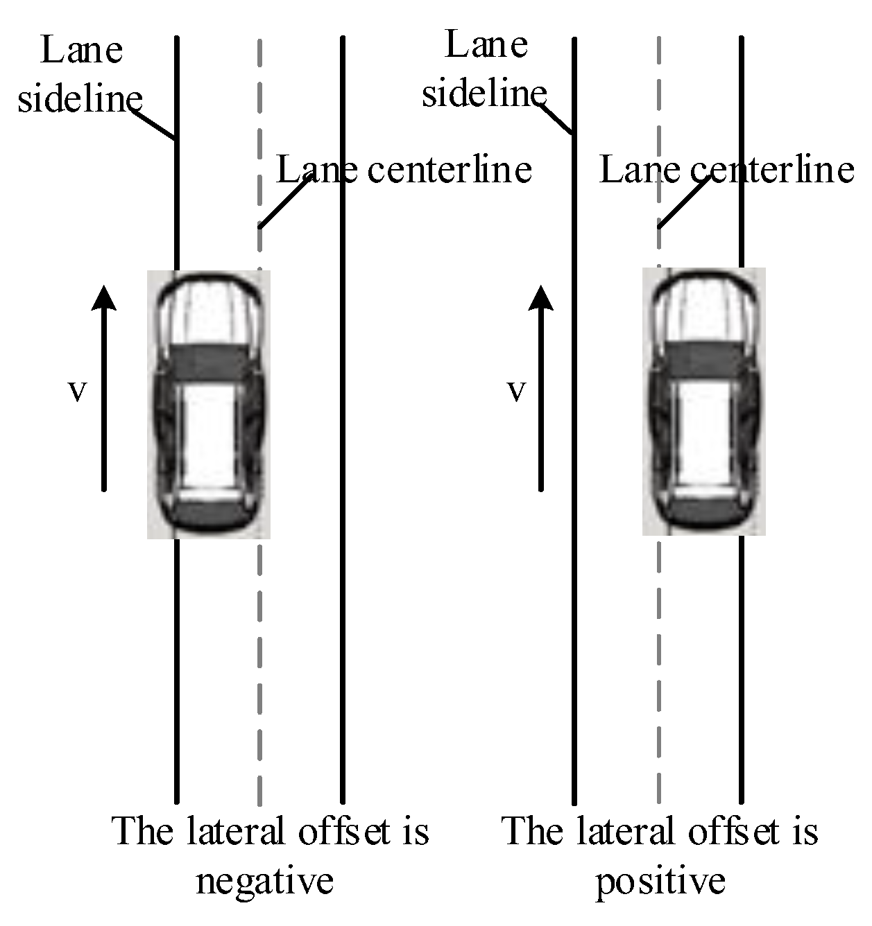
- Lateral offset
- (5)
- Driver’s emergency response
3. Data Analysis and Results
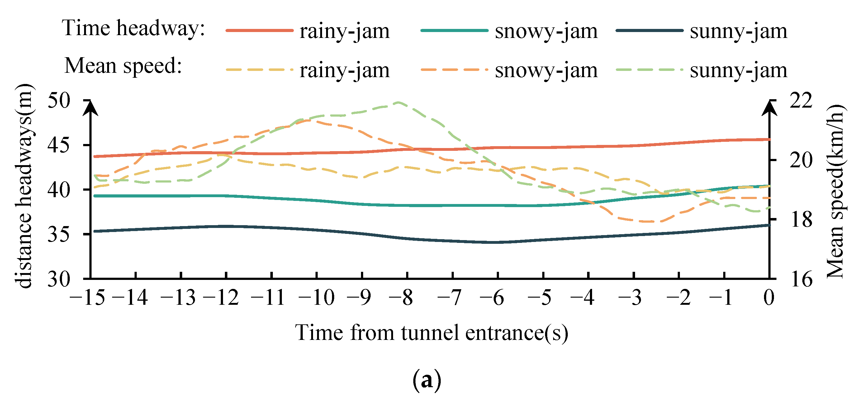
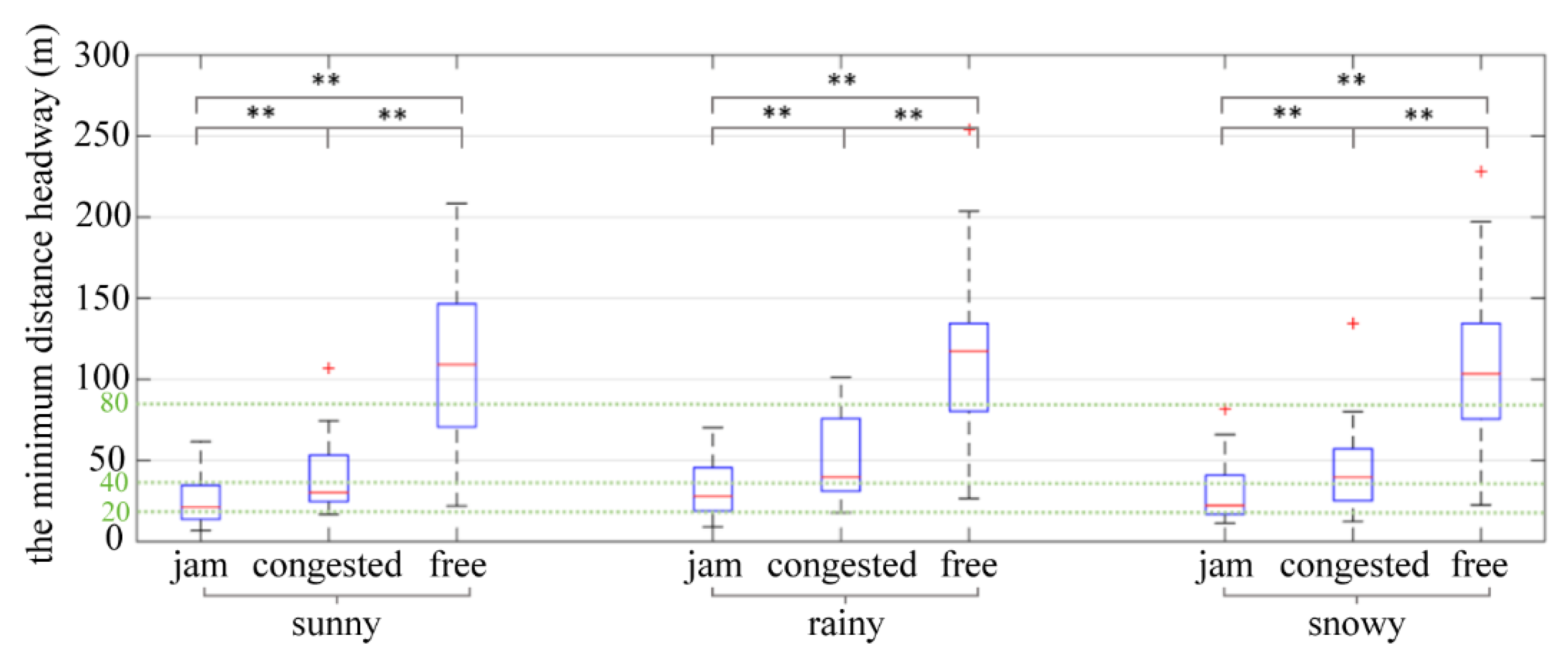
3.1. The Influence of Different Conditions on Distance Headways
3.2. The Influence of Different Conditions on Time Headways
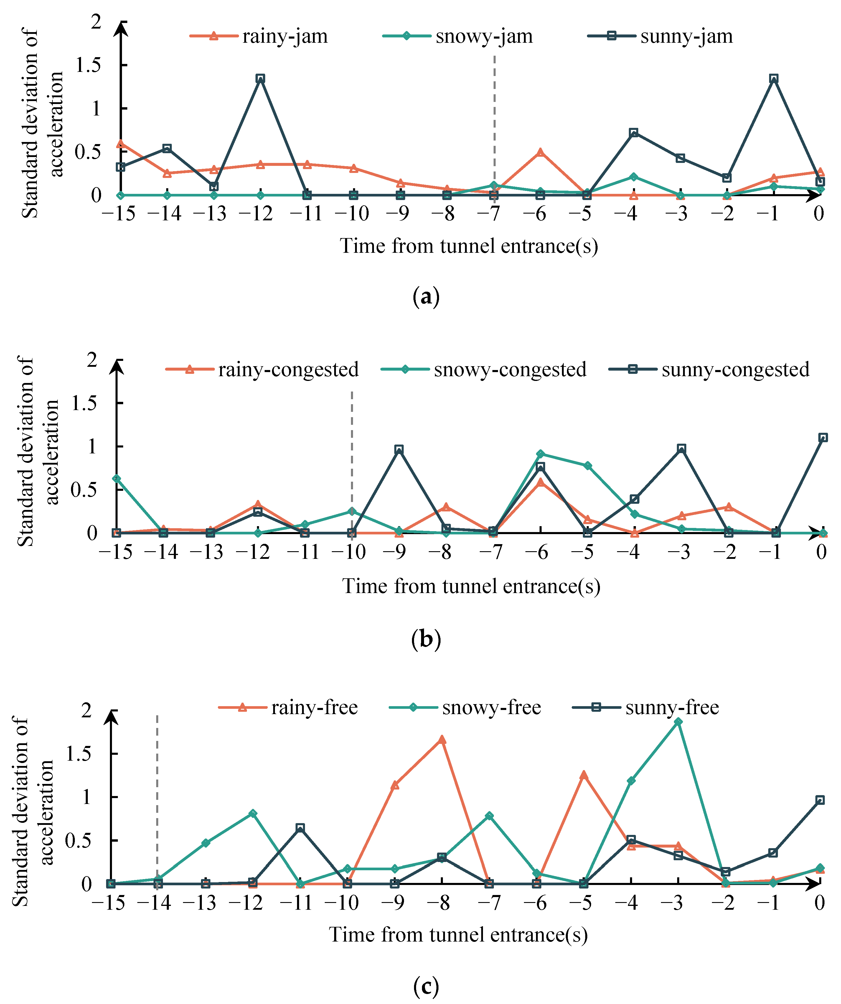
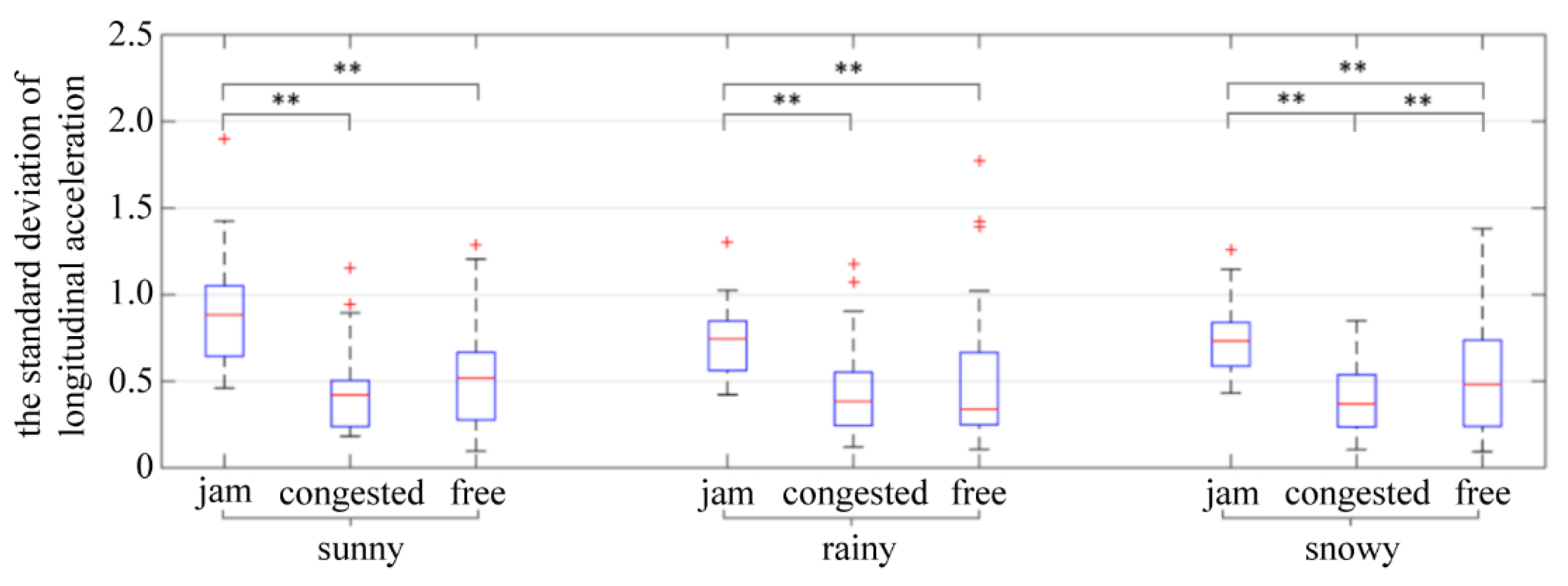
3.3. The Influence of Different Conditions on Drivers’ Acceleration Behavior
3.4. The Influence of Different Conditions on Lateral Offset
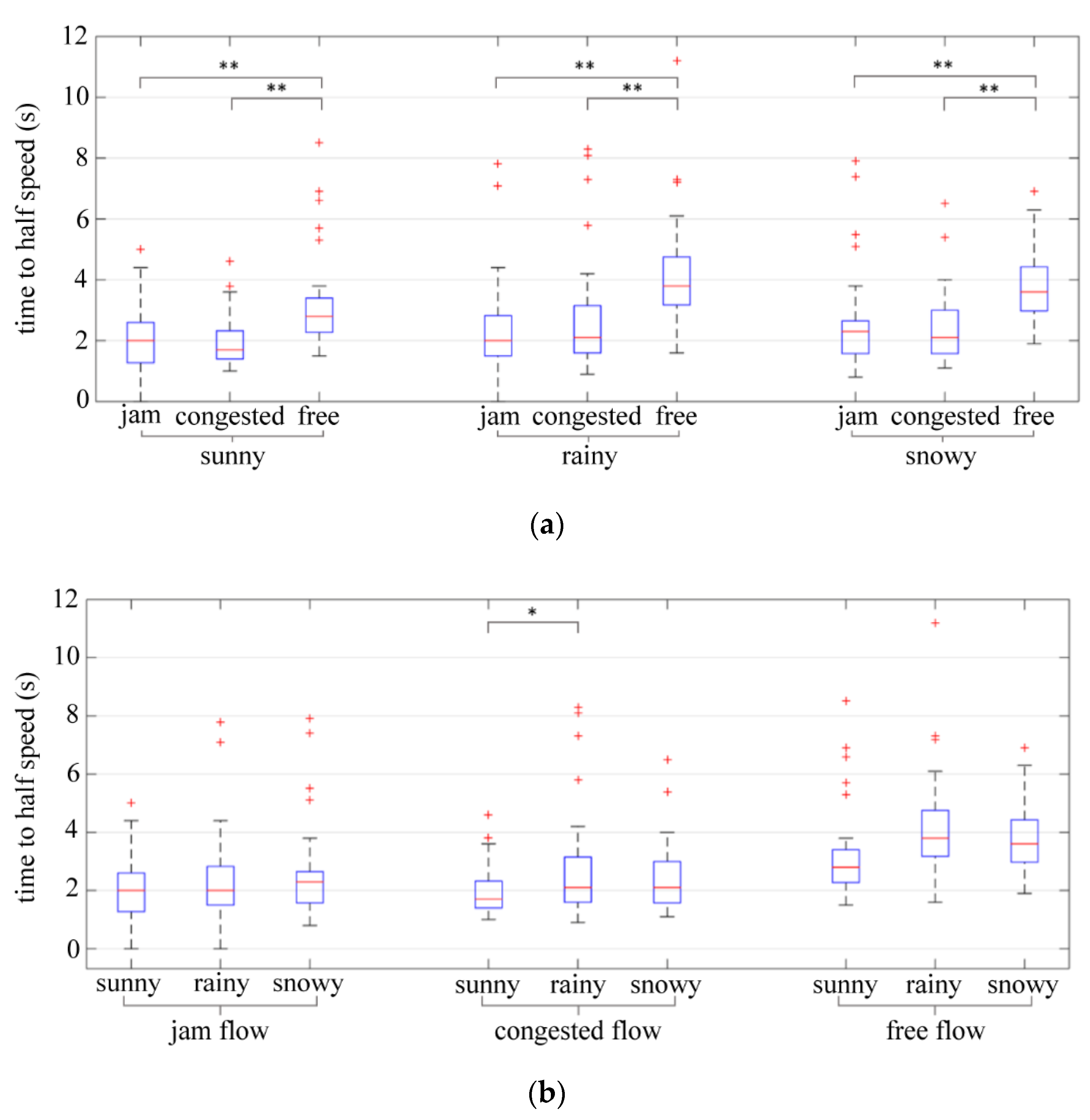
3.5. The Influence of Different Conditions on Driver’s Emergency Response Time
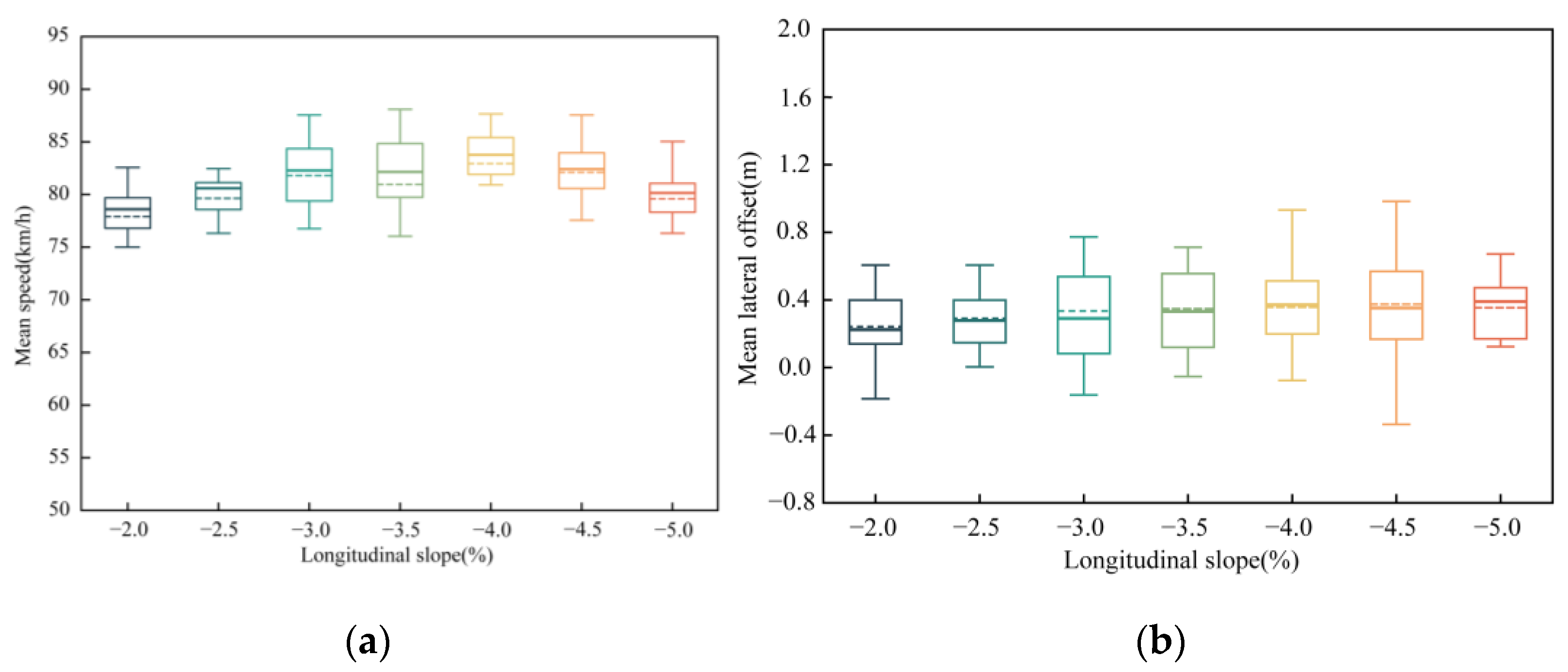
3.6. The Influence of Different Slopes on Driving Behaviors
4. Conclusions
Author Contributions
Funding
Institutional Review Board Statement
Informed Consent Statement
Data Availability Statement
Conflicts of Interest
References
- Chen, S.; Chen, Y.; Xing, Y. Comparison and Analysis of Crash Frequency and Rate in Cross-River Tunnels Using Random-Parameter Models. J. Transp. Saf. Secur. 2020, 14, 280–304. [Google Scholar] [CrossRef]
- Amundsen, F.H.; Ranes, G. Studies on Traffic Accidents in Norwegian Road Tunnels. Tunn. Undergr. Space Technol. 2000, 15, 3–11. [Google Scholar] [CrossRef]
- Yeung, J.S.; Wong, Y.D. Road Traffic Accidents in Singapore Expressway Tunnels. Tunn. Undergr. Space Technol. 2013, 38, 534–541. [Google Scholar] [CrossRef]
- Caliendo, C.; Gugliemo, M.; Guida, M. Comparison and Analysis of Road Tunnel Traffic Accident Frequencies and Rates using Random-Parameter Models. J. Transp. Saf. Secur. 2016, 8, 177–195. [Google Scholar] [CrossRef]
- Shao, X.J.; Chen, F.; Ma, X.X.; Pan, X.D. The Impact of Lighting and Longitudinal Slope on Driver Behavior in Cross-river and cross-sea tunnels: A Simulator Study. Tunn. Undergr. Space Technol. 2022, 122, 104367. [Google Scholar] [CrossRef]
- Akamtsu, M.; Imachou, N.; Sasaki, Y. Simulator Study on Driver’s Behavior While Driving Through a Tunnel in a Rolling Area. Driv. Simul. Conf. 2003, 10, 1–14. [Google Scholar]
- Wang, Y.; Kong, L.Q.; Guo, Z.Y.; Han, C.L. Alignment Design at Tunnel Entrance and Exit Zone Based on Operating Safety. J. Highw. Transp. Res. Dev. 2008, 25, 134–138. [Google Scholar]
- Wan, H.; Du, Z.; Ran, B. Speed Control Method for Highway Tunnel Safety Based on Visual Illusion. Transp. Res. Rec. J. Transp. Res. Board 2015, 2485, 1–7. [Google Scholar] [CrossRef]
- Shi, H.; Tu, Z.H.; Gao, K. Analysis of Car Following Behaviors Under Hazy Weather Conditions Based on High Fidelity Driving Simulator. J. Tongji Univ. 2018, 46, 326–333. [Google Scholar]
- Kang, J.; Ni, R.; Andersen, G.J. Effects of Reduced Visibility from Fog on Car-Following Performance. Transp. Res. Rec. J. Transp. Res. Board 2008, 2069, 9–15. [Google Scholar] [CrossRef]
- Ibrahim, A.T.; Hall, F.L. Effect of Adverse Weather Conditions on Speed-Flow-Occupancy Relationships. J. Transp. Res. Board 1994, 1457, 184–191. [Google Scholar]
- Rosey, F.; Aillerie, I.; Espié, S.; Vienne, F. Driver Behavior in Fog Is Not only A Question of Degraded Visibility—A Simulator Study. Saf. Sci. 2017, 95, 50–61. [Google Scholar] [CrossRef]
- Minderhoud, M.M.; Zuurbier, F. Empirical Data on Driving Behavior in Stop-And-Go Traffic. IEEE Intell. Veh. Symp. 2004, 6, 676–681. [Google Scholar]
- Piao, J.; McDonald, M. Low Speed Car Following Behavior from Floating Vehicle Data. IEEE Intell. Veh. Symp. 2003, 6, 462–467. [Google Scholar]
- Zhao, X.; Ren, G.; Chen, C. Comprehensive Effects of Adverse Weather on Drivers Car-Following Behavior Based on Driving Simulation Technology. J. Chongqing Jiaotong Univ. 2019, 38, 90–95. [Google Scholar]
- The Ministry of Public Security of the People’s Republic of China. Regulations Governing Management of Highways in the People’s Republic of China; The Ministry of Public Security of the People’s Republic of China: Beijing, China, 2009. [Google Scholar]
- Wang, Y.Z.; Hu, J.M.; Li, L.; Zhang, Y. Optimal Coordination of Variable Speed Limit to Eliminate Freeway Wide Moving Jams. Int. J. Mod. Phys. C 2014, 25, 1450038. [Google Scholar] [CrossRef]
- Zhou, W.; Zhang, S.R. Analysis of Distance Headway. J. Southeast Univ. 2003, 19, 378. [Google Scholar]
- Chen, Z.; Wen, H.Y. Modeling car-following model with comprehensive safety field in freeway tunnels. J. Transp. Eng. Part A Syst. 2022, 148, 04022040. [Google Scholar] [CrossRef]
- Feng, Z.X.; Yang, M.M.; Zhang, W.H. Effect of longitudinal slope of urban underpass tunnels on drivers’ heart rate and speed: A study based on a real vehicle experiment. Tunn. Undergr. Space Technol. 2018, 81, 525–533. [Google Scholar] [CrossRef]


| Traffic | Free Flow | Congested Flow | Jam Flow | |
|---|---|---|---|---|
| Weather | ||||
| sunny weather | sunny-free | sunny-congested | sunny-jam | |
| rainy weather | rainy-free | rainy-congested | rainy-jam | |
| snowy weather | snowy-free | snowy-congested | snowy-jam | |
| Weather Condition | Rainfall Coefficient | Snowfall Coefficient | Adhesion Reduction Coefficient | |
|---|---|---|---|---|
| Inside the Tunnel | Outside the Tunnel | |||
| sunny weather | - | - | 1.00 | 1.00 |
| rainy weather | 0.6 | - | 1.00 | 0.60 |
| snowy weather | - | 0.45 | 1.00 | 0.45 |
| Traffic Condition | Speed (km/h) | Number | Significance |
|---|---|---|---|
| congested | 19.27 | 838 | 0.0068 ** |
| jam | 40.85 | 513 |
| Classification | Variable | Unit |
|---|---|---|
| System Variable | Time | s |
| road variable | Road abscissa | m |
| Road angle | ° | |
| Road Id/Lane Id | - | |
| Lane type | - | |
| Intersection Id | - | |
| vehicle variable | Speed/X/Y | km·h−1 |
| Acceleration/X/Y | m·s−2 | |
| Lane gap/Road gap | m | |
| Yaw speed | (°)·s−1 | |
| Yaw acceleration | (°)·s−2 | |
| Car Spacing | m | |
| Speed Difference | km·h−1 | |
| Driver Operation Data | Steering at steering rack | ° |
| Steering wheel speed | (°)·s−1 | |
| Gas pedal | - | |
| Brake pedal force | daN |
| Weather Condition | Variance Homogeneity Test | Mean Test | Post-Hoc | |||
|---|---|---|---|---|---|---|
| ANOVA | Welch ANOVA | Comparison Item | LSD | Games-Howell | ||
| sunny | 0.000 ** | - | 0.000 ** | Jam < Congested | - | 0.005 ** |
| Congested < Free | - | 0.000 ** | ||||
| Jam < Free | - | 0.000 ** | ||||
| rainy | 0.000 ** | - | 0.000 ** | Jam < Congested | - | 0.008 ** |
| Congested < Free | - | 0.000 ** | ||||
| Jam < Free | - | 0.000 ** | ||||
| snowy | 0.000 ** | - | 0.000 ** | Jam < Congested | - | 0.022 ** |
| Congested < Free | - | 0.000 ** | ||||
| Jam < Free | - | 0.000 ** | ||||
| Weather Condition | Variance Homogeneity Test | Mean Test | Post-Hoc | |||
|---|---|---|---|---|---|---|
| ANOVA | Welch ANOVA | Comparison Item | LSD | Games-Howell | ||
| sunny | 0.000 ** | - | 0.023 ** | Jam < Congested | - | 0.315 |
| Congested < Free | - | 0.171 | ||||
| Jam < Free | - | 0.036 ** | ||||
| rainy | 0.000 ** | - | 0.009 ** | Jam < Congested | - | 0.903 |
| Congested < Free | - | 0.007 ** | ||||
| Jam < Free | - | 0.014 ** | ||||
| snowy | 0.000 ** | - | 0.002 ** | Jam < Congested | - | 0.186 |
| Congested < Free | - | 0.177 | ||||
| Jam < Free | - | 0.003 ** | ||||
| Weather Condition | Variance Homogeneity Test | Mean Test | Post-Hoc | |||
|---|---|---|---|---|---|---|
| ANOVA | Welch ANOVA | Comparison Item | LSD | Games-Howell | ||
| sunny | 0.302 | 0.042 ** | - | Jam < Congested | 0.431 | - |
| Congested < Free | 0.014 ** | - | ||||
| Jam < Free | 0.089 * | - | ||||
| rainy | 0.170 | 0.232 | - | - | - | - |
| snowy | 0.186 | 0.349 | - | - | - | - |
| Traffic Condition | Variance Homogeneity Test | Mean Test | Post-Hoc | |||
|---|---|---|---|---|---|---|
| ANOVA | Welch ANOVA | Comparison Item | LSD | Games-Howell | ||
| Jam | 0.502 | 0.090 * | - | sunny < rainy | 0.047 ** | - |
| snowy < rainy | 0.355 | - | ||||
| sunny < snowy | 0.281 | - | ||||
| Congested | 0.237 | 0.346 | - | - | - | - |
| Free | 0.966 | 0.712 | - | - | - | - |
| Weather Condition | Variance Homogeneity Test | Mean Test | Post-Hoc | |||
|---|---|---|---|---|---|---|
| ANOVA | Welch ANOVA | Comparison Item | LSD | Games-Howell | ||
| sunny | 0.000 ** | - | 0.000 ** | Jam < Congested | - | 0.000 ** |
| Congested < Free | 0.035 ** | |||||
| Jam < Free | 0.000 ** | |||||
| rainy | 0.000 ** | - | 0.000 ** | Jam < Congested | - | 0.000 ** |
| Congested < Free | 0.233 | |||||
| Jam < Free | 0.000 ** | |||||
| snowy | 0.000 ** | - | 0.000 ** | Jam < Congested | - | 0.000 ** |
| Congested < Free | 0.031 ** | |||||
| Jam < Free | 0.000 ** | |||||
| Weather Condition | Variance Homogeneity Test | Mean Test | Post-Hoc | |||
|---|---|---|---|---|---|---|
| ANOVA | Welch ANOVA | Comparison Item | LSD | Games-Howell | ||
| sunny | 0.171 | 0.000 ** | - | Jam < Congested | 0.000 ** | - |
| Congested < Free | 0.351 | - | ||||
| Jam < Free | 0.000 ** | - | ||||
| rainy | 0.004 ** | - | 0.000 ** | Jam < Congested | - | 0.000 ** |
| Congested < Free | - | 0.778 | ||||
| Jam < Free | - | 0.030 ** | ||||
| snowy | 0.001 ** | - | 0.000 ** | Jam < Congested | - | 0.000 ** |
| Congested < Free | - | 0.027 ** | ||||
| Jam < Free | - | 0.004 ** | ||||
| Weather Condition | Variance Homogeneity Test | Mean Test | Post-Hoc | |||
|---|---|---|---|---|---|---|
| ANOVA | Welch ANOVA | Comparison Item | LSD | Games-Howell | ||
| sunny | 0.019 ** | - | 0.006 ** | Jam < Congested | - | 0.612 |
| Congested < Free | - | 0.036 ** | ||||
| Jam < Free | - | 0.004 ** | ||||
| rainy | 0.001 ** | - | 0.000 ** | Jam < Congested | - | 0.683 |
| Congested < Free | - | 0.000 ** | ||||
| Jam < Free | - | 0.000 ** | ||||
| snowy | 0.294 | 0.000 ** | - | Jam < Congested | 0.862 | - |
| Congested < Free | 0.000 ** | - | ||||
| Jam < Free | 0.000 ** | - | ||||
| Weather Condition | Variance Homogeneity Test | Mean Test | Post-Hoc | |||
|---|---|---|---|---|---|---|
| ANOVA | Welch ANOVA | Comparison Item | LSD | Games-Howell | ||
| sunny | 0.036 ** | - | 0.002 ** | Jam < Congested | - | 0.913 |
| Congested <Free | - | 0.008 ** | ||||
| Jam < Free | - | 0.002 ** | ||||
| rainy | 0.988 | 0.000 ** | - | Jam < Congested | 0.980 | - |
| Congested <Free | 0.000 ** | - | ||||
| Jam < Free | 0.000 ** | - | ||||
| snowy | 0.443 | 0.001 ** | - | Jam < Congested | 0.663 | - |
| Congested <Free | 0.002 ** | - | ||||
| Jam < Free | 0.001 ** | - | ||||
| Weather Condition | Variance Homogeneity Test | Mean Test | Post-Hoc | |||
|---|---|---|---|---|---|---|
| ANOVA | Welch ANOVA | Comparison Item | LSD | Games-Howell | ||
| sunny | 0.015 ** | - | 0.000 ** | Jam < Congested | - | 0.961 |
| Congested < Free | - | 0.000 ** | ||||
| Jam < Free | - | 0.001 ** | ||||
| rainy | 0.822 | 0.009 ** | - | Jam < Congested | 0.930 | - |
| Congested < Free | 0.009 ** | - | ||||
| Jam < Free | 0.007 ** | - | ||||
| snowy | 0.658 | 0.000 ** | - | Jam < Congested | 0.713 | - |
| Congested < Free | 0.000 ** | - | ||||
| Jam < Free | 0.000 ** | - | ||||
| Traffic Condition | Variance Homogeneity Test | Mean Test | Post-Hoc | |||
|---|---|---|---|---|---|---|
| ANOVA | Welch ANOVA | Comparison Item | LSD | Games-Howell | ||
| Jam | 0.133 | 0.250 | - | - | - | - |
| Congested | 0.012 ** | - | 0.031 ** | sunny < rainy | - | 0.070 * |
| snowy < rainy | - | 0.699 | ||||
| sunny < snowy | - | 0.124 | ||||
| Free | 0.768 | 0.117 | - | - | - | - |
| Variables | SS | df | MS | F Value | p Value | |
|---|---|---|---|---|---|---|
| Speed | Variance between groups | 580.186 | 6 | 96.697 | 8.889 | 1.198 × 10⁻⁸ |
| Intraclass variance | 2284.424 | 210 | 10.878 | |||
| Lateral offset | Variance between groups | 0.744 | 6 | 0.124 | 1.77 | 0.106 |
| Intraclass variance | 14.695 | 210 | 0.069 |
Publisher’s Note: MDPI stays neutral with regard to jurisdictional claims in published maps and institutional affiliations. |
© 2022 by the authors. Licensee MDPI, Basel, Switzerland. This article is an open access article distributed under the terms and conditions of the Creative Commons Attribution (CC BY) license (https://creativecommons.org/licenses/by/4.0/).
Share and Cite
Zhang, T.; Chen, F.; Huang, Y.; Song, M.; Hu, X. Analysis of Car-Following Behaviors under Different Conditions on the Entrance Section of Cross-River and Cross-Sea Tunnels: A Case Study of Shanghai Yangtze River Tunnel. Int. J. Environ. Res. Public Health 2022, 19, 11975. https://doi.org/10.3390/ijerph191911975
Zhang T, Chen F, Huang Y, Song M, Hu X. Analysis of Car-Following Behaviors under Different Conditions on the Entrance Section of Cross-River and Cross-Sea Tunnels: A Case Study of Shanghai Yangtze River Tunnel. International Journal of Environmental Research and Public Health. 2022; 19(19):11975. https://doi.org/10.3390/ijerph191911975
Chicago/Turabian StyleZhang, Ting, Feng Chen, Yadi Huang, Mingtao Song, and Xiao Hu. 2022. "Analysis of Car-Following Behaviors under Different Conditions on the Entrance Section of Cross-River and Cross-Sea Tunnels: A Case Study of Shanghai Yangtze River Tunnel" International Journal of Environmental Research and Public Health 19, no. 19: 11975. https://doi.org/10.3390/ijerph191911975
APA StyleZhang, T., Chen, F., Huang, Y., Song, M., & Hu, X. (2022). Analysis of Car-Following Behaviors under Different Conditions on the Entrance Section of Cross-River and Cross-Sea Tunnels: A Case Study of Shanghai Yangtze River Tunnel. International Journal of Environmental Research and Public Health, 19(19), 11975. https://doi.org/10.3390/ijerph191911975