
Statistical Methods for Assessing the Explained Variation of a Health Outcome by a Mixture of Exposures


Abstract
:1. Introduction
2. Material and Methods
2.1. Estimation of the Total Effects of Exposures
2.2. Decorrelation of the Exposures with Possibly Supplementary Exposure Data
2.3. Confounder Adjustment and the Variation Explained by a Subset of Exposures
2.4. Estimation of the Total Interaction Effects
2.5. Inference on the Explained Variation
- Compute estimator using one of the proposed methods based on data . Denote the estimate by .
- Permute the outcome , to , where is a randomly selected permutation of indices . Compute estimator using the same method based on permuted data . Denote the estimate by .
- Repeat step 2 for times. The estimated p-value is the frequency of , i.e.,
- Compute estimator using one of the proposed methods based on data . Denote the estimate by .
- Permute the covariates , to , where is a random selected permutation of indices . Compute estimator by the same method based on the permuted data . Denote the estimate by .
- Repeat step 2 for times. The estimated p-value is the frequency of , i.e.,
2.6. R Package: TEV
2.7. Simulation Study Design
2.8. Data Analysis Approach
3. Results
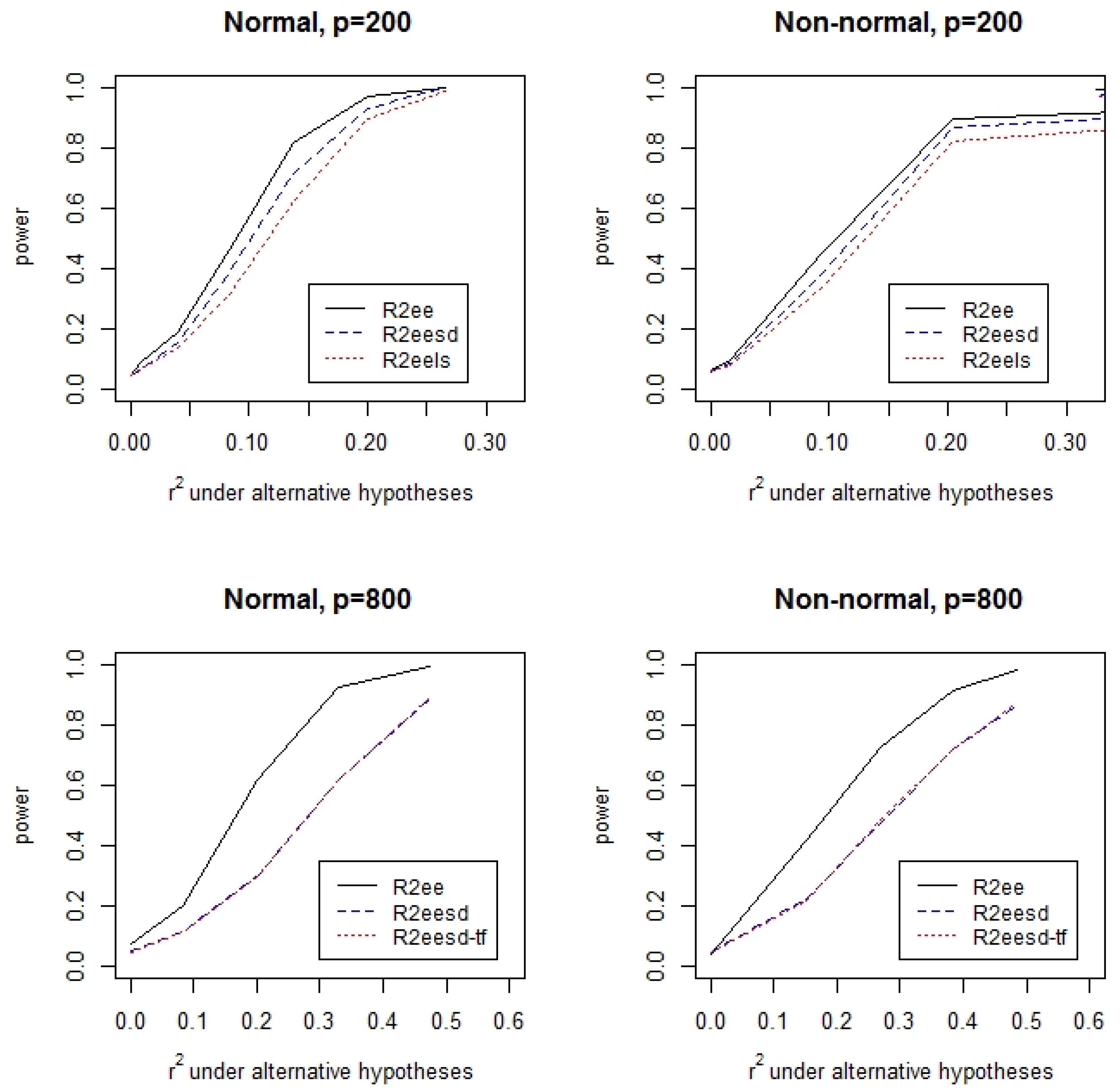
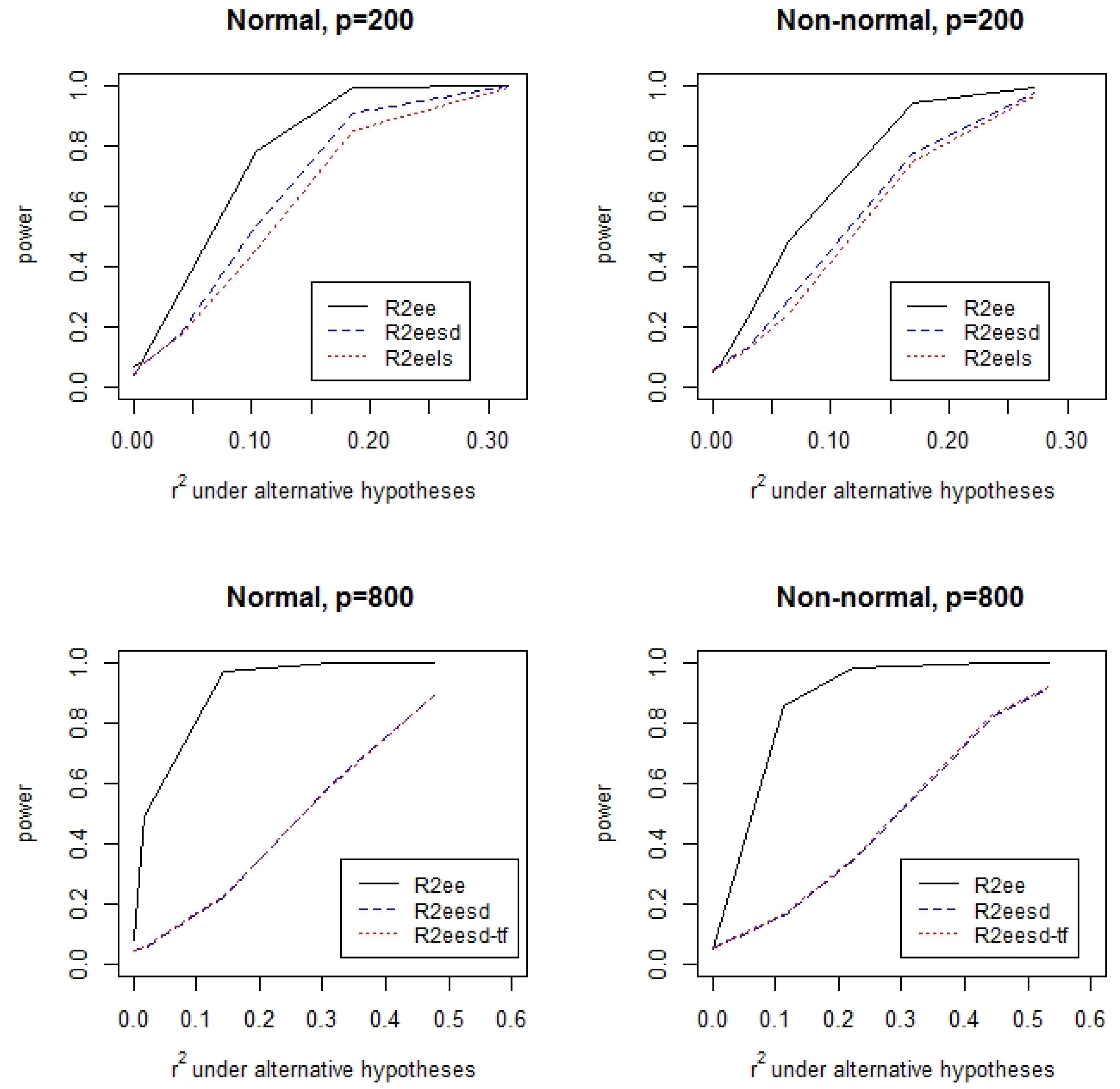
3.1. Simulations
3.2. Data Analysis
4. Discussion
5. Conclusions
Author Contributions
Funding
Institutional Review Board Statement
Informed Consent Statement
Data Availability Statement
Acknowledgments
Conflicts of Interest
Appendix A
References
- Billionnet, C.; Sherrill, D.; Annesi-Maesano, I. Estimating the Health Effects of Exposure to Multi-Pollutant Mixture. Ann. Epidemiol. 2012, 22, 126–141. [Google Scholar] [CrossRef] [PubMed]
- Lazarevic, N.; Barnett, A.G.; Sly, P.D.; Knibbs, L.D. Statistical Methodology in Studies of Prenatal Exposure to Mixtures of Endocrine-Disrupting Chemicals: A Review of Existing Approaches and New Alternatives. Environ. Health Perspect. 2019, 127, 026001. [Google Scholar] [CrossRef] [PubMed]
- Zou, H.; Hastie, T.; Tibshirani, R. Sparse principal component analysis. J. Comput. Graph. Stat. 2006, 15, 265–286. [Google Scholar] [CrossRef] [Green Version]
- Tibshirani, R. Regression Shrinkage and Selection via the Lasso. J. R. Stat. Soc. Ser. B (Methodol.) 1996, 58, 267–288. [Google Scholar] [CrossRef]
- Zou, H.; Hastie, T. Regularization and variable selection via the elastic net. J. R. Stat. Soc. Ser. B 2005, 67, 301–320. [Google Scholar] [CrossRef] [Green Version]
- Helland, I.S. On the structucre of partial least squares regression. Commun. Stat. Simul. Comput. 1988, 18, 581–607. [Google Scholar] [CrossRef]
- Stone, M.; Brooks, R. Continuum regression: Cross-validation sequantially constructed predictionembracing ordinary least square, partial least square and principal component regression. J. R. Stat. Soc. Ser. B 1990, 52, 237–269. [Google Scholar] [CrossRef]
- Garthwaite, P.H. An interpretation of partial least squares. J. Am. Stat. Assoc. 1994, 89, 122–127. [Google Scholar] [CrossRef]
- Chun, H.; Keles, S. Sparse partial least squares regression for simultaneous dimension reduction and variable selection. J. R. Stat. Soc. Ser. B 2010, 72, 3–25. [Google Scholar] [CrossRef] [Green Version]
- Benjamini, Y.; Yu, B. The schuffle estimator for explainable variance in fmri experiments. Ann. Appl. Stat. 2013, 7, 2007–2033. [Google Scholar] [CrossRef] [Green Version]
- Guo, Z.; Wang, W.; Cai, T.T.; Li, H. Optimal estimation of co-heritability in high-dimensional linear models. J. Am. Stat. Assoc. 2018, 114, 358–369. [Google Scholar] [CrossRef]
- Verzelen, N.; Gassiat, E. Adaptive estimation of high-dimensional signal-to-noise ratios. Bernoulli 2018, 24, 3683–3710. [Google Scholar] [CrossRef] [Green Version]
- Cai, T.T.; Guo, Z. Semi-supervised inference for explained variance in high-dimensional regression and its applications. J. R. Stat. Soc. Ser. B 2020, 82, 391–419. [Google Scholar]
- Yang, J.; Benyamin, B.; McEvoy, B.P.; Gordon, S.; Henders, A.; Nyholt, D.; A Madden, P.; Heath, A.C.; Martin, N.; Montgomery, G.; et al. Common SNPs explain a large proportion of the heritability for human height. Nat. Genet. 2010, 42, 565–569. [Google Scholar] [CrossRef] [PubMed] [Green Version]
- Dicker, L.H. Variance estimation in high-dimensional linear models. Biometrika 2014, 101, 269–284. [Google Scholar] [CrossRef]
- Janson, L.; Barber, R.F.; Candès, E. EigenPrism: Inference for high dimensional signal-to-noise ratios. J. R. Stat. Soc. Ser. B Stat. Methodol. 2016, 79, 1037–1065. [Google Scholar] [CrossRef] [Green Version]
- Chen, H.Y. Statistical inference on explained variation in high-dimensional linear model with dense effects. arXiv 2021, arXiv:2201.08723. [Google Scholar]
- Pavuk, M.; Serio, T.C.; Cusack, C.; Cave, M.; Rosenbaum, P.F.; Birnbaum, L. Hypertension in Relation to Dioxins and Polychlorinated Biphenyls from the Anniston Community Health Survey Follow-Up. Environ. Health Perspect. 2019, 127, 127007. [Google Scholar] [CrossRef]
- Everett, C.J.; Mainous, A.G., III; Frithsen, I.L.; Player, M.S.; Matheson, E.M. Association of polychlorinated biphenyls with hypertension in the 1999–2002 National Health and Nutrition Examination Survey. Environ. Res. 2008, 108, 94–97. [Google Scholar] [CrossRef]
- Raffetti, E.; Donato, F.; De Palma, G.; Leonardi, L.; Sileo, C.; Magoni, M. Polychlorinated biphenyls (PCBs) and risk of hypertension: A population-based cohort study in a Northern Italian highly polluted area. Sci. Total Environ. 2020, 714, 136660. [Google Scholar] [CrossRef]
- Goncharov, A.; Pavúk, M.; Foushee, H.R.; Carpenter, D.O. Blood Pressure in Relation to Concentrations of PCB Congeners and Chlorinated Pesticides. Environ. Health Perspect. 2011, 119, 319–325. [Google Scholar] [CrossRef] [PubMed]
- Valera, B.; Ayotte, P.; Poirier, P.; Dewailly, E. Associations between plasma persistent organic pollutant levels and blood pressure in Inuit adults from Nunavik. Environ. Int. 2013, 59, 282–289. [Google Scholar] [CrossRef] [PubMed]
- Bai, Z.D.; Silverstein, J.W. Spectral Analysis of Large Dimensional Random Matrices. Available online: https://link.springer.com/book/10.1007/978-1-4419-0661-8 (accessed on 30 December 2021).
- Schweiger, R.; Kaufman, S.; Laaksonen, R.; Kleber, M.E.; Marz, W.; Eskin, E.; Rosset, S.; Halperin, E. Fats and accurate construction of confidence intervals for heritability. Am. J. Hum. Genet. 2016, 98, 1181–1192. [Google Scholar] [CrossRef] [PubMed] [Green Version]
- van Buuren, S.; Groothuis-Oudshoorn, K. Mice: Multivariate Imputation by Chained Equations inR. J. Stat. Softw. 2011, 45, 1–67. [Google Scholar] [CrossRef] [Green Version]
- Tobin, M.D.; Sheehan, N.; Scurrah, K.J.; Burton, P.R. Adjusting for treatment effects in studies of quantitative traits: Antihypertensive therapy and systolic blood pressure. Stat. Med. 2005, 24, 2911–2935. [Google Scholar] [CrossRef]
- Balakrishnan, P.; Beaty, T.; Young, J.H.; Colantuoni, E.; Matsushita, K. Methods to estimate underlying blood pressure: The Atherosclerosis Risk in Communities (ARIC) Study. PLoS ONE 2017, 12, e0179234. [Google Scholar] [CrossRef]
- Kumar, S.K.; Feldman, M.W.; Rehkopf, D.H.; Tuljapurkar, S. Limitations of GCTA as a solution to the missing heritability problem. Proc. Natl. Acad. Sci. USA 2016, 113, E61–E70. [Google Scholar] [CrossRef] [Green Version]


| Tests | N,I | N,M | N,H | C,I | C,M | C,H | |
|---|---|---|---|---|---|---|---|
| (400, 200) | R2ee | 0.044 | 0.053 | 0.068 | 0.063 | 0.059 | 0.050 |
| R2eesd | 0.046 | 0.059 | 0.040 | 0.056 | 0.049 | 0.055 | |
| R2eels | 0.046 | 0.052 | 0.044 | 0.061 | 0.050 | 0.057 | |
| (400, 800) | R2ee | 0.075 | 0.050 | 0.082 | 0.041 | 0.057 | 0.054 |
| R2eesd | 0.054 | 0.048 | 0.048 | 0.047 | 0.051 | 0.051 | |
| R2eesd-tf | 0.046 | 0.046 | 0.045 | 0.048 | 0.057 | 0.059 |
| Covariates | Model ) | Method | Empirical Variance | Averaged 95% CI | 95% CI Coverage | 95%CI Length | ||
|---|---|---|---|---|---|---|---|---|
| (400, 200) | Independ. | Normal | EigenPrism | 0.000 | 0.0031 | (0.263, 0.503) | 97.4% | 0.240 |
| (0.401) | GCTA | 0.005 | 0.0030 | (0.272, 0.510) | 96.5% | 0.238 | ||
| R2ee | 0.000 | 0.0029 | (0.300, 0.501) | 94.1% | 0.202 | |||
| R2eels | 0.003 | 0.0031 | (0.285, 0.522) | 91.7% | 0.237 | |||
| R2eesd | 0.001 | 0.0029 | (0.298, 0.507) | 94.5% | 0.209 | |||
| EigenPrism | −0.004 | 0.0050 | (0.284, 0.517) | 89.3% | 0.233 | |||
| (0.421) | GCTA | −0.003 | 0.0050 | (0.293, 0.528) | 89.9% | 0.235 | ||
| R2ee | −0.003 | 0.0047 | (0.248, 0.589) | 97.6% | 0.342 | |||
| R2eels | −0.001 | 0.0050 | (0.241, 0.608) | 94.0% | 0.367 | |||
| R2eesd | −0.001 | 0.0048 | (0.253, 0.589) | 97.1% | 0.336 | |||
| Correlated | Normal | EigenPrism | −0.002 | 0.0027 | (0.328, 0.547) | 95.7% | 0.219 | |
| (0.455) | GCTA | −0.017 | 0.0024 | (0.313, 0.547) | 97.6% | 0.234 | ||
| R2ee | −0.020 | 0.0016 | (0.367, 0.506) | 89.3% | 0.139 | |||
| R2eels | −0.002 | 0.0026 | (0.348, 0.560) | 92.3% | 0.212 | |||
| R2eesd | −0.003 | 0.0026 | (0.356, 0.551) | 93.8% | 0.195 | |||
| EigenPrism | 0.017 | 0.0052 | (0.300, 0.527) | 86.3% | 0.228 | |||
| (0.413) | GCTA | −0.003 | 0.0049 | (0.285, 0.520) | 90.5% | 0.236 | ||
| R2ee | −0.002 | 0.0035 | (0.231, 0.593) | 97.8% | 0.362 | |||
| R2eels | 0.020 | 0.0052 | (0.255, 0.617) | 89.7% | 0.362 | |||
| R2eesd | 0.019 | 0.0051 | (0.267, 0.597) | 93.8% | 0.331 | |||
| (400, 800) | Independ. | Normal | EigenPrism | −0.001 | 0.0103 | (0.160, 0.646) | 98.5% | 0.485 |
| (0.403) | R2ee | −0.006 | 0.0097 | (0.207, 0.589) | 94.9% | 0.382 | ||
| R2eesd | 0.021 | 0.0217 | (0.146, 0.726) | 95.5% | 0.580 | |||
| EigenPrism | 0.001 | 0.0129 | (0.183, 0.668) | 97.0% | 0.485 | |||
| (0.423) | R2ee | −0.005 | 0.0129 | (0.182, 0.661) | 96.2% | 0.479 | ||
| R2eesd | 0.013 | 0.0251 | (0.135, 0.770) | 96.0% | 0.635 | |||
| Correlated | Normal | EigenPrism | −0.361 | 0.0036 | (0.000, 0.313) | 13.4% | 0.313 | |
| (0.410) | R2ee | 0.034 | 0.0029 | (0.349, 0.538) | 82.0% | 0.189 | ||
| R2eesd | 0.020 | 0.0217 | (0.151, 0.730) | 94.8% | 0.579 | |||
| EigenPrism | −0.335 | 0.0034 | (0.000, 0.306) | 18.8% | 0.306 | |||
| (0.380) | R2ee | 0.048 | 0.0050 | (0.214,0.645) | 94.9% | 0.431 | ||
| R2eesd | 0.033 | 0.0251 | (0.117,0.748) | 95.8% | 0.631 |
| Tests | N,I | N,I | C,I | C,I | N,H | N,H | C,H | C,H |
|---|---|---|---|---|---|---|---|---|
| 0 | 0.198 | 0 | 0.195 | 0 | 0.212 | 0 | 0.322 | |
| R2ee | 0.015 | 0.065 | 0.055 | 0.050 | 0.105 | 0.005 | 0.075 | 0.005 |
| R2eesd | 0.030 | 0.045 | 0.065 | 0.055 | 0.045 | 0.015 | 0.070 | 0.045 |
| R2eels | 0.035 | 0.025 | 0.060 | 0.060 | 0.055 | 0.006 | 0.040 | 0.040 |
| Continuous Variable | Range | Mean | Standard Deviation |
|---|---|---|---|
| Age (in years) | Min = 20, Max = 85 | 51.82 | 18.59 |
| BMI | Min = 16.07, Max = 62.99 | 28.43 | 5.98 |
| Alcohol drinks/year | Min = 0, Max = 365 | 48.13 | 90.36 |
| Categorical variable | Categories | Counts | Frequencies |
| Gender | Male | 1667 | 0.51 |
| Female | 1595 | 0.49 | |
| Race | Mexican American | 733 | 0.22 |
| Other Hispanic | 132 | 0.04 | |
| Non-Hispanic White | 1722 | 0.53 | |
| Non-Hispanic Black | 573 | 0.18 | |
| Other race | 102 | 0.03 | |
| Education | Less than high school | 1060 | 0.32 |
| High school diploma | 766 | 0.23 | |
| More than high school | 1436 | 0.44 | |
| Poverty/income ratio | Less than 1.3 | 886 | 0.27 |
| Between 1.3 and 3.5 | 1321 | 0.40 | |
| More than 3.5 | 1055 | 0.32 | |
| Smoke status | Never | 1637 | 0.5 |
| Former | 975 | 0.3 | |
| Current | 650 | 0.2 | |
| Taken hormones modifying drugs last month | Yes | 584 | 0.18 |
| No | 2678 | 0.82 | |
| Taken adrenal cortical steroids drugs last month | Yes | 74 | 0.02 |
| No | 3188 | 0.98 | |
| Taken antidiabetic drugs last month | Yes | 304 | 0.09 |
| No | 2958 | 0.91 | |
| Taken immunosuppressant drugs last month | Yes | 16 | 0.005 |
| No | 3246 | 0.995 |
| Outcome | Interaction | Method | Unadjusted | 95% CI | Adjusted * | p-Value |
|---|---|---|---|---|---|---|
| SBP | No | EigenPrism | 0.348 | (0.314, 0.379) | ||
| GCTA | 0.348 | (0.276, 0.417) | ||||
| R2ee | 0.351 | (0.319, 0.382) | 0.036 | 0.0044 | ||
| R2eels | 0.348 | (0.313, 0.383) | 0.033 | 0.0044 | ||
| Yes | EigenPrism | 0.479 | (0.398, 0.544) | |||
| GCTA | 0.349 | (0.297, 0.403) | ||||
| R2ee | 0.349 | (0.306, 0.392) | 0.000 ** | 0.090 | ||
| R2eels | 0.480 | (0.413, 0.548) | 0.132 ** | <0.031 | ||
| DBP | No | EigenPrism | 0.060 | (0.012, 0.105) | ||
| GCTA | 0.073 | (0.046, 0.105) | ||||
| R2ee | 0.073 | (0.021, 0.126) | 0.034 | 0.0045 | ||
| R2eels | 0.061 | (0.013, 0.108) | 0.023 | 0.0044 | ||
| Yes | EigenPrism | 0.275 | (0.158, 0.369) | |||
| GCTA | 0.121 | (0.072, 0.173) | ||||
| R2ee | 0.121 | (0.054, 0.189) | 0.048 ** | <0.031 | ||
| R2eels | 0.277 | (0.179, 0.375) | 0.216 ** | <0.031 |
Publisher’s Note: MDPI stays neutral with regard to jurisdictional claims in published maps and institutional affiliations. |
© 2022 by the authors. Licensee MDPI, Basel, Switzerland. This article is an open access article distributed under the terms and conditions of the Creative Commons Attribution (CC BY) license (https://creativecommons.org/licenses/by/4.0/).
Share and Cite
Chen, H.Y.; Li, H.; Argos, M.; Persky, V.W.; Turyk, M.E. Statistical Methods for Assessing the Explained Variation of a Health Outcome by a Mixture of Exposures. Int. J. Environ. Res. Public Health 2022, 19, 2693. https://doi.org/10.3390/ijerph19052693
Chen HY, Li H, Argos M, Persky VW, Turyk ME. Statistical Methods for Assessing the Explained Variation of a Health Outcome by a Mixture of Exposures. International Journal of Environmental Research and Public Health. 2022; 19(5):2693. https://doi.org/10.3390/ijerph19052693
Chicago/Turabian StyleChen, Hua Yun, Hesen Li, Maria Argos, Victoria W. Persky, and Mary E. Turyk. 2022. "Statistical Methods for Assessing the Explained Variation of a Health Outcome by a Mixture of Exposures" International Journal of Environmental Research and Public Health 19, no. 5: 2693. https://doi.org/10.3390/ijerph19052693