Article

Computational Study of Thermal Comfort and Reduction of CO2 Levels inside a Classroom

by
Guillermo Efren Ovando-Chacon
1,
Abelardo Rodríguez-León
1,*,
Sandy Luz Ovando-Chacon
2,*,
Martín Hernández-Ordoñez
1,
Mario Díaz-González
1 and
Felipe de Jesús Pozos-Texon
1
1
Tecnológico Nacional de México, Instituto Tecnológico de Veracruz, Calzada Miguel Ángel de Quevedo 2779, Veracruz 91860, Mexico
2
Tecnológico Nacional de México, Instituto Tecnológico de Tuxtla Gutiérrez, Carretera Panamericana km 1080, Tuxtla Gutierrez 29000, Mexico
*
Authors to whom correspondence should be addressed.
Int. J. Environ. Res. Public Health 2022, 19(5), 2956; https://doi.org/10.3390/ijerph19052956
Submission received: 20 January 2022 / Revised: 22 February 2022 / Accepted: 1 March 2022 / Published: 3 March 2022

Abstract

:
Due to the current COVID-19 pandemic, guaranteeing thermal comfort and low CO2 levels in classrooms through efficient ventilation has become vitally important. This study presents three-dimensional simulations based on computational fluid dynamics of airflow inside an air-conditioned classroom located in Veracruz, Mexico. The analysis included various positions of an air extractor, Reynolds numbers up to 3.5 × 10⁴, four different concentrations of pollutant sources, and three different times of the day. The simulations produced velocity, air temperature, and CO2 concentrations fields, and we calculated average air temperatures, average CO2 concentrations, and overall ventilation effectiveness. Our results revealed an optimal extractor position and Reynolds number conducive to thermal comfort and low CO2 levels due to an adequate ventilation configuration. At high pollutant concentrations, it is necessary to reduce the number of students in the classroom to achieve safe CO2 levels.

1. Introduction

Over the past twenty years, in the context of climate change associated with the use of energy obtained from fossil fuels, many studies on non-isothermal flows in spaces have addressed the problem of how to achieve thermal comfort while optimizing energy use. However, these studies should also take into account air quality, especially in closed spaces where large numbers of people are present, often involving high CO2 values (above 1000 ppm) as a product of human activity and poor air circulation. Before the SARS-CoV-2 pandemic, millions of students around the world attended classrooms requiring energy-efficient ventilation systems that guaranteed thermal comfort and low levels of pollutants, such as CO2. The above was necessary since comfortable and healthy conditions in closed spaces, such as classrooms, favor the learning process because they prevent inattention or drowsiness. However, the pandemic has made it more imperative than ever to ensure low levels of CO2 since this parameter can serve as an indicator of the risk of contagion among the academic community in schools, universities, and other higher education institutions. The problem is more serious when high CO2 concentrations occur in closed spaces, such as classrooms, where students and teachers are together for long periods [1,2,3,4], putting their health at risk and significantly reducing student achievement [1].
Therefore, during the last decade, several studies indirectly [5,6,7,8,9] or directly [1,10,11,12] focused on the problem of pollutant concentration and thermal comfort in closed spaces. All of the research focusing indirectly on excess CO2 (or other contaminants) approaches the problem by using numerical studies in cavities, namely computational fluid dynamics (CFD) simulations [5,6,7,9,13]. Although these are excellent theoretical works, these studies are characterized by not having a direct application to a problem in a defined space in the real world. Research directly focusing on excess CO2 analyzes existing closed spaces for human use in the real world. Some of these studies represent strictly applied research, such as [10], in which the effect of CO2 sensors was studied to improve the performance of forced convection ventilation systems. On the other hand, studies such as [11,14,15,16,17,18,19,20,21] were conducted in real spaces, such as industrial buildings for welding processes, hospitals, computer laboratories, offices, mosques, kitchens, buildings, dorm rooms, or schools.
Other studies have focused explicitly on excess CO2 in educational spaces [1,2,3,4,12,22,23,24]. Of these, several experimental studies, such as [1,2,3,4], measure CO2 concentrations in academic settings using different methods. A remarkable case is [2]; in addition to controlling contamination by CO2, the authors sought specifically to reduce the transmission of SARS-CoV-2 in the educational environments using experimental measurements to infer the behavior of the fluid in the closed space and established a correlation between ventilation aimed at improving air quality and the decrease in contagions. A detailed study of airflow behavior in a closed space using CFD allows a better understanding of the phenomenon to achieve good air circulation that reduces CO2 and, incidentally, contributes to lowering the SARS-CoV-2 contagion rate. Similarly, ref. [25] conducted a study to understand ozone distribution in closed spaces using CFD simulations in turbulent flow regimes to predict ozone levels in a SARS-CoV-2-disinfected area.
Until now, there are very few CFD studies in schools where thermal comfort is analyzed considering a large number of students; in [26,27], classrooms without air conditioning and with open windows were studied. On the other hand, other CFD studies inside spaces have considered the transport of particles to study the transmission of contagious diseases in schools [28,29] and hospitals [30,31,32,33].
Most of the numerical studies on indoor CO2 concentration published so far have been based on simple geometry and a pollutant source in the walls, and only a few have considered a large number of people inside the space. On the other hand, none of these studies have considered the flux of heat through closed windows of an air-conditioned classroom. Due to the above, it is of great importance to determine how the position of a ceiling extractor affects the thermal comfort conditions and the CO2 values in an air-conditioned classroom with students. The purpose of the present study is to perform numerical simulations in a three-dimensional geometry; to know the effects of extractor position and Reynolds numbers on the ventilation; and to find a configuration that guarantees thermal comfort and low CO2 levels in an air-conditioned classroom for various concentrations of pollutant sources and different heat fluxes. In the analyzed classroom, thirty students and one teacher were considered. In Mexico and especially in places with a hot climate, such as the port of Veracruz, many public schools have poorly designed air-conditioning systems. This causes a deficient removal of CO2, and for this reason, it is necessary to know the specific flow pattern inside the classrooms to find the proper arrangement of the equipment that guarantees better air quality.

2. Methodology

2.1. Physical Model

Figure 1 shows the undergraduate classroom (X002) analyzed in the present study. The classroom is located in building “X” of the Department of Mechanical Engineering of the Tecnológico Nacional de México, Campus Veracruz, located in the port of Veracruz, México, where warm climate prevails. The study considered 30 students and one teacher inside the space. The west wall has two closed windows, one measuring 2.2 m × 2 m and the other 1.5 m × 2 m, through which there are heat gains inside the room, mainly after 11:00 a.m., due to solar radiation. It is important to note that the windows cannot be opened, so they always remain closed. The east wall was considered to be at a constant temperature of 25 °C. The south wall is exposed to the outside and is in front of a tall building that shades it most of the day; meanwhile, the north wall adjoins another classroom. The south and north walls are considered adiabatic. Air-conditioning equipment (440–1150 m3/h) was available in the classroom at the top center of the ceiling and near the south wall. Figure 2a shows a plan view of the classroom, building “X”, and its surroundings. The classroom’s door is in the west wall, which adjoins a common hall that connects with other classrooms and the rest of the building; the door is usually closed during classes. On the other hand, the main doors of the building are typically locked during the day, opening and closing only to allow teachers and students to access or exit the building; as a consequence, the air inside the building, especially in the most crowded classrooms, is very poor. Therefore, it is necessary to propose improvements to reduce CO2 concentration in the classrooms. In the present study, three-dimensional numerical simulations of airflow and energy and mass transport were carried out inside the classroom previously described. The analysis was performed for different Reynolds numbers (Re) in the range of 1000 to 35,000, with CO2 sources (Cs) from 35,000 ppm to 42,500 ppm, generated by the students and the teacher and distributed in the classroom. The heat fluxes imposed through the classroom windows were 95.8 W/m2, 326.6 W/m2, and 147.6 W/m2, which correspond to three different hours of the day: 11:30 a.m., 3:30 p.m., and 6:30 p.m., respectively. An air extractor was installed to reduce CO2 concentration levels inside the room, and the effect of eight different positions of this device, as shown in Figure 2b, was analyzed. The simulations were performed for inlet velocities in the range of 0.21–1.46 m/s, with inlet temperature of 22 °C and CO2 concentration of 340 ppm. Persons were considered inside the room with a heat flux of 75 W. The study considered a production of CO2 per occupant in the range of 9.456 × 10⁻⁶ kg/s to 1.20 2 × 10⁻⁵ kg/s.
The analyzed classroom is located in a recently created building where undergraduate classes took place from January 2019 to 23 March 2020, when classes were interrupted as an official health measure mandated by the federal government of Mexico to reduce the spread of COVID-19. The classrooms located in this building lack an efficient ventilation system. In addition, due to the warm climate in the city of Veracruz, the building and the classrooms are fully air-conditioned. Therefore, the doors and windows remain closed all day. Consequently, CO2 concentrations are high at almost all times. In June 2019, different measurements were taken inside the classroom, observing that during the class that started at 11:00 a.m., CO2 concentration increased rapidly above 10:00 ppm, while pollutant concentrations decreased below 1000 ppm in the class that started at 7:00 p.m. Due to the fact that all the classes have a duration of 1 h, the study was carried out in the middle of the class that started at 11:00 a.m., that is, at 11:30 a.m., and in the middle of the previous class at 7:00 p.m., that is, at 6:30 p.m. On the other hand, the measurements indicated that the maximum heat flux through the closed windows of the classroom occurred during the 3:00 pm class; therefore, the study was carried out in the middle of that class, that is, at 3:30 p.m.
To solve the problem of high concentrations of CO2, the thermal behavior of the air flow and the concentration of the pollutant in the classroom were analyzed through numerical simulations for different conditions of heat transfer through the closed windows, which correspond to three different hours of the day. The simulations provide velocity, temperature, and CO2 concentration fields, average temperatures and CO2 concentrations in the classroom, and overall ventilation effectiveness for air temperature distribution and overall ventilation effectiveness for CO2 removal.

2.2. Governing Equations

Turbulent flow, CO2 distribution, and temperature inside a classroom subject to thermal loads and sources of pollutant are described by Navier–Stokes, mass transport, energy, and turbulence equations. The steady-state approach was used successfully by other researchers to study the concentration of CO2 in indoor spaces [5,6,7,34]. The steady-state governing equations used in this work are:
ρ u i u j x j = p x i + x j μ u i x j + u j x i ρ u i ´ u j ´ ¯ + F i
ρ u i x i = 0
ρ C p u j T x j = x j λ T x j ρ C p u i ´ T ´ ¯
u j C x j = x j D C x j u i ´ C ´ ¯
where ui is the i component of the velocity, xi is the i component of the spatial coordinate, ρ is the density, p is the pressure, µ is the dynamic viscosity, Fi is the i component of the body force, T is the temperature, Cp is the specific heat, λ is the thermal conductivity, C is the concentration, and D is the diffusion coefficient. The properties of the air–CO2 mixture are shown in Table 1.
In Equations (1)–(4), the Reynolds stress tensor, turbulent heat flux, and turbulent mass flow can be approximated by:
ρ u i ´ u j ´ ¯ = μ t u i x j + u j x i + 2 3 ρ K δ ij
ρ u i ´ T ´ ¯ = μ t Pr t T x j
u i ´ C ´ ¯ = μ t Sc t C x j
where Prt is the turbulent Prandtl number, and Sct is the turbulent Schmidt number. On the other hand, the body force can be described as follows:
F i = ρ g δ 2 j β T T T ref + β C C C ref
The coefficients of thermal expansion βT and of concentration βC are calculated by βT = 1/T0 y βC = 1/C0, where T0 = 296 K and C0 = 340 ppm; g is the gravity acceleration. The turbulent kinetic energy K and the turbulent kinetic energy dissipation ε are calculated by:
ρ u i K x i = x i μ + μ t σ K K x i + P K + G K ρ ε
ρ u i ϵ x i = x i μ + μ t σ ε ε x i + C ϵ 1 ϵ K P K + C ϵ 3 G K C ϵ 2 ρ ε 2 K
In the previous equations, PK is the turbulent kinetic energy production rate, GK is the generation or destruction of turbulence due to fluctuations in body forces, and µt is the turbulent viscosity. The coefficients values for the turbulence model are Cε1 = 1.44, Cε2 = 1.92, Cε3 = tanh|u3/u1|, σk = 1.0, and σε = 1.3. PK and GK can be calculated as follow:
P K = μ t u i x j + u j x i u i x j
G K = β T g μ t σ T T x j δ 2 j
μ t = C μ ρ K 2 ε

2.3. Overall Ventilation Effectiveness Equations

In addition to the average air temperature and the average concentration of CO2 in the interior of the space, calculated using the temperature and concentration fields obtained by the governing equations, it is important to quantify how the comfort temperature and the contaminant are distributed in the analyzed space. In this regard, Awbi [35] established that an efficient ventilation system is a result of good air quality and good thermal comfort and proposed Equation (14) to define overall ventilation effectiveness for air temperature distribution and Equation (15) to define the overall ventilation effectiveness for CO2 removal:
E T = T out T in T A T in
E C = C out C in C A C in
In the above equations, Tout and Cout are temperature and CO2 concentration at the outlet, respectively. Tin and Cin are, respectively, temperature and CO2 concentration at the inlet. TA and CA are, respectively, temperature and CO2 concentration averages inside the room.

2.4. Numerical Method

The governing equations are solved using the finite element method [36,37]. The scalar variables are calculated in the main mesh, while the velocity components are calculated in another mesh, which is twice finer than the main mesh. The discretization is carried out by means of an operator separation scheme that decouples the non-linearity of the Navier–Stokes equations. This scheme allows to solve the conservation equations by the following subproblems:
Ω u i x i ψ d Ω = 0
Ω u j u i x j ψ d Ω = Ω P n Ψ x i d Ω
Ω u j T x j ψ d Ω + Ω λ ρ · C p T x j Ψ x j d Ω Ω μ t ρ · Pr t T x j Ψ x i d Ω = Γ T D Ψ d Γ
Ω u j C x j ψ d Ω + Ω D C x j Ψ x j d Ω Ω μ t Sc t C x j Ψ x i d Ω = Γ C D Ψ d Γ
Ω μ + μ t u i x j Ψ x j d Ω = Ω 2 3 ρ K δ ij Ψ d Ω + Ω F i Ψ d Ω + Γ u i D Ψ d Γ
Ω u j K x j ψ d Ω + Ω μ + μ t σ K K x j Ψ x j d Ω = Ω P K ψ d Ω + Ω G K ψ d Ω Ω ρ ϵ ψ d Ω
Ω u j ϵ x j ψ d Ω + Ω μ + μ t σ ε ϵ x j Ψ x j d Ω = Ω ϵ K C ϵ 1 P K + C ϵ 3 G K ψ d Ω Ω ρ ϵ K C ϵ 2 ϵ ψ d Ω
The appropriate mesh size is obtained by a mesh sensitivity study in which the behavior of the average temperature inside the classroom is analyzed for six different mesh sizes with the following node numbers: 255825, 350340, 462348, 550220, 650450, 751825, and 849246. Table 2 shows the behavior of average air temperature convergence for different cases. The maximum difference in the average air temperatures between the two finer meshes is 0.28 °C for case III, 6:30 p.m., Cs = 37,500 ppm, and Re = 15,000. The simulations were carried out by applying mesh refinement towards the walls in order to have greater precision in these regions (see Figure 3). The steady-state simulations were obtained when the consecutive values of each variable were less than 10−6. The spatial discretization was of the order of 0.01 m.

2.5. Validation

To demonstrate precision and validate the obtained calculations, we solved the problem of turbulent natural convection in a square cavity with air. This turbulent natural convection problem was experimentally studied by Ampofo and Karayiannis [38]. In Figure 4a, the average temperature profiles in the transverse central plane of the cavity are compared for Rayleigh numbers of Ra = 1.58 × 10⁹. Additionally, the problem of turbulent flow was solved in a cavity with two differentially heated opposite vertical walls as proposed by Saury et al. [39]. In Figure 4b, the local Nusselt numbers in the hot wall are compared for Ra = 1.2 × 10¹¹.
On the other hand, experimental measurements of the indoor air temperature of the classroom were also made. Table 3 shows comparisons between these values for Case III, 6:30 p.m., Cs = 37,500 ppm, Re = 15,000. The maximum error of the numerical results compared to the experimental results was 2.4%. These comparisons show that the numerical code used in this study can solve turbulent flow problems. The numerical code was developed using the Fortran programming language, in the thermofluid group of the Technological Institute of Veracruz. The numerical code has previously been used to solve various thermofluid problems [40,41,42,43].

3. Results and Discussion

3.1. Velocity Fields

Figure 5 presents velocity fields for two different extractor positions at 3:30 p.m. for Re = 15,000 and Cs = 37,500 ppm. Figure 5a shows the airflow patterns when the extractor is located in the corner formed by the wall with windows and the wall near the air-conditioning supply. In this case, the air-conditioning supply and the exhaust through the extractor are located on the same side. The flow patterns for this configuration show better air distribution inside the classroom, as the airflow circulates from the center of the south wall moving toward the east wall, then proceeds to the north wall, where it changes direction toward the west wall; and when it collides with this last wall, the airflow changes direction again toward the south wall, where it finally rises toward the extractor. Therefore, the air sweep for this case was the most effective since it covers all classroom areas. Figure 5b describes the behavior of the airflow inside the classroom when the extractor is located in the corner formed by the wall that contains the door and the wall opposite to the air-conditioning supply. In this case, the flow dynamics show that the air-conditioning stream is divided into two flows: one of them directed toward the west (hot) wall, which is the most intense, and the other, less intense stream moves toward the east (cold) wall. Subsequently, both streams move toward the north wall; the stream traveling along the east wall has a short trajectory since, when it collides with the north wall, it changes direction, moving toward the extractor in the ceiling. On the other hand, the stream that travels along the west wall has a long trajectory since, when it collides with the north wall, it travels along this entire wall until it reaches the east wall, where it rises toward the extractor. In this case, the air-conditioning supply and the exhaust of the extractor are located on opposite sides. As a result, the air sweep over the hot wall is more intense and has a longer trajectory, transporting a large amount of energy from the window into the classroom.

3.2. Temperatures Fields

To analyze the thermal behavior inside the classroom, Figure 6 describes the temperature fields for two different positions of the extractor at 3:30 p.m., Re = 15,000, and Cs = 37,500 ppm. Figure 6a presents the distribution of the air temperature inside the classroom when the extractor is located in the corner formed by the wall with windows and the wall near the air-conditioning system. A low temperature can be observed in the center of the classroom due to the cold air stream supplied by the air conditioning. The temperature tends to increase toward the side walls, where the windows and the door are located. However, this increase is greater on the west wall due to the heat flux transmitted by the windows, which are struck by the sun’s rays. The best distribution of cold air flow occurs when the extractor is on the same side as the air-conditioning system. On the other hand, the most adverse temperature field occurs when the extractor is located in the corner formed by the wall that contains the door and the wall opposite to the air-conditioning system (Figure 6b); in this case, significant temperature increases are observed even near the eastern wall. In addition, this configuration results in the largest reduction in the size of the cold region in the center of the classroom. In this configuration the extractor is placed on the side of the cold wall and away from the supply of the air-conditioning system.
According to these data, the case where the size of the cold central region is larger occurs when the extractor is located on the same side as the air-conditioning system and near the hot window, which is related to the fact that, in this case, air distribution is the most effective, covering all of the classroom zones. Furthermore, the case where the air temperature inside the classroom is kept less uniform and warmer in the central part occurs when the extractor is located on the opposite side of the air-conditioning system and close to the cold wall, which is related to the fact that, in this case, a sizeable part of the airflow follows a long trajectory along the west (hot) wall, transporting a large amount of energy into the classroom.

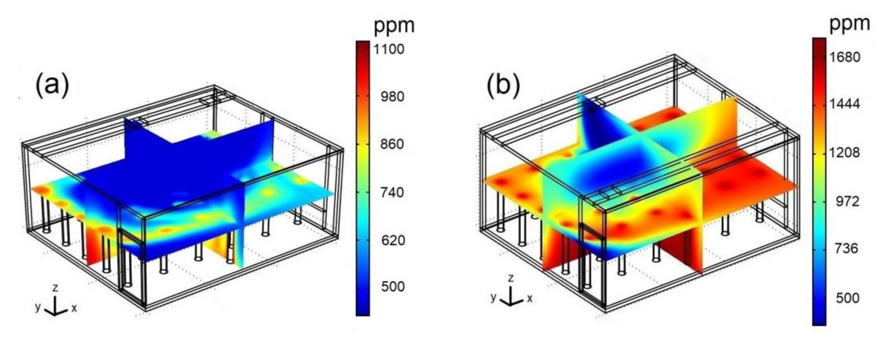
3.3. CO2 Concentration Fields

For a general idea of the spatial distribution of the pollutant inside the classroom, Figure 7 shows CO2 concentration fields for two different positions of the extractor at 3:30 p.m., Re = 15,000, and Cs = 37,500 ppm. The case where most of the classroom’s interior has low CO2 concentrations occurs when the extractor is located in the corner formed by the wall that contains the windows and the wall closest to the supply of the air-conditioning system (see Figure 7a). The worst configuration, with extensive high-CO2 regions, is when the extractor is located in the corner formed by the wall that contains the door and the wall opposite the air-conditioning system as shown in Figure 7b. In this case, significant increases in CO2 concentration are observed throughout the XY plane, while the only low-CO2 concentration region is the top center of the classroom.
In general, when the extractor is placed on the west wall (hot) side, CO2 concentrations decrease considerably, especially when the extractor is placed on the same side as the air-conditioning system (see Figure 7a). On the other hand, CO2 concentrations are very high in most of the classroom area when the extractor is placed on the east wall (cold) side, mainly when the extractor is placed opposite to the air-conditioning system (see Figure 7b).

3.4. Average Air Temperature

In the area of Veracruz, where the analyzed classroom is located, the climate is warm most of the year; accordingly, most people are used to the high-temperature environment. In this study, we considered the comfort temperature between 24.0 °C and 25.5 °C. When the temperature drops below the lower limit, most people start to feel cold. Furthermore, the greater the difference in temperature between indoor areas with air conditioning and outdoors, the greater the possibility of becoming sick due to sudden temperature changes.
Figure 8 shows the average temperatures TA of air inside the classroom for three hours of the day as a function of the Reynolds number with different extractor locations and different concentrations Cs of pollutant sources. Figure 8a,b shows the cases at 11:30 a.m. for Cs = 35,000 ppm and Cs = 42,500 ppm, respectively. The minimum temperature values are TA= 24.19 °C for Cs = 35,000 ppm and TA = 24.52 °C for Cs = 42,500 ppm. The maximum values are TA= 27.82 °C for Cs = 35,000 ppm and TA= 28.44 °C for Cs = 42,500 ppm.
Figure 8c,d shows the cases at 3:30 p.m. for Cs = 35,000 ppm and Cs = 42,500 ppm, respectively. The minimum temperature values are TA = 24.88 °C for Cs = 35,000 ppm and TA = 25.23 °C for Cs = 42,500 ppm. The maximum values are TA= 30.23 °C for Cs = 35,000 ppm and TA = 30.48 °C for Cs = 42,500 ppm.
Figure 8e,f shows the cases at 6:30 p.m. for Cs = 35,000 ppm and Cs = 42,500 ppm, respectively. The minimum temperature values are TA = 24.50 °C for Cs = 35,000 ppm and TA = 25.01 °C for Cs = 42,500 ppm. The maximum values are TA = 29.23 °C for Cs = 35,000 ppm and TA = 29.74 °C for Cs = 42,500 ppm. All these minimum values are within the thermal comfort range and correspond to configuration III and Re = 15,000, while the maximum values occur for configuration IV and Re = 1000.

3.5. Overall Ventilation Effectiveness for Air Temperature Distribution

Since the dynamics of airflow inside the classroom varies in each configuration, changing the spatial distribution of the temperature, it is necessary to evaluate overall ventilation effectiveness for temperature air temperature distribution ET. The higher the parameter value, the more homogeneous the interior temperature since the airflow improves heat removal. To analyze the effect of the Reynolds number on air temperature distribution inside the classroom, Figure 9 shows the ET at different extractor positions and different concentration Cs of pollutant sources at 11:30 a.m., 3:30 p.m., and 6:30 p.m., respectively.
Figure 9a,b shows the cases at 11:30 a.m. for Cs = 35,000 ppm and Cs = 42,500 ppm, respectively. The maximum values of ET, where the most homogeneous air temperature distribution inside the classroom is guaranteed, are ET = 20.78 and 24.43 for Cs = 35,000 and 42,500 ppm, respectively.
At 3:30 p.m., the maximum values are ET = 25.28 (Figure 9c) and 27.68 (Figure 9d) for Cs = 35,000 and 42,500 ppm, respectively. Figure 9e,f shows the cases at 6:30 p.m. for Cs = 35,000 ppm and Cs = 42,500 ppm, respectively. The maximum values of ET are 23.90 and 26.27 for Cs = 35,000 and 42,500 ppm, respectively. For the three times of the day considered, the maximum values occur for configuration III and Re = 15,000, which coincides with the condition where minimum TA values are obtained.
The most favorable cases, where the temperature is within the range of thermal comfort, and the air temperature distribution is more homogeneous, occur for case III, which corresponds to the configuration where the air extractor is located on the same side as the air conditioning system’s air inlet and near the hot window. On the other hand, the configurations with the highest temperatures and the most unfavorable temperature distribution with low ET values occur for case VI, when the extractor is located in the corner furthest from the air inlet of the air-conditioning system and close to the cold inner wall. Furthermore, the path of the air stream since supplied by the air-conditioning system to its exit through the extractor has a substantial effect on air temperature distribution: in all cases, the lowest average air temperature values and the maximum ET values were observed for Re = 15,000. The highest values of average air temperature and the minimum ET values were observed for Re = 1000. At low velocities, air temperature distribution is heterogeneous; however, as the velocity increases, the distribution becomes more homogeneous, reaching an optimal value when Re = 15,000.

3.6. Average CO2 Concentration

In general, safe limits of CO2 concentration are considered to be between 700 ppm and 1000 ppm. In this study, the safe limit of average CO2 concentration CA inside the classroom was considered below 700 ppm, which guarantees a pleasant space where students can carry out their activities. Although analyzing the contagion of a disease requires more complex models that take into account the transport of exhaled droplets, the level of CO2 can be a practical measure in classrooms to reduce the risk of contagion since high levels of CO2 are an indication of agglomerations. Recent publications report that the concentration of CO2 in classrooms can help reduce the risk of transmission of contagious diseases, such as SARS-CoV-2, since low levels of CO2 indicate clean air [2,44,45,46,47].
Figure 10, Figure 11 and Figure 12 show average concentrations of CA pollutant inside the classroom as a function of Reynolds number for different extractor locations and different concentrations Cs of pollutant sources. In general, it can be observed that the configurations where contaminant concentrations are lower occurred for case III, that is, when the air inlet and outlet are on the same side. On the other hand, the most unfavorable configurations occur in case VI, when the air inlet and outlet are on opposite sides. Air velocity has another significant effect on average pollutant concentration inside the classroom, observing in all cases: minimum average CO2 concentrations occurred for Re = 15,000, while the maximum values occurred for Re = 1000. This implies that, at low velocities, the release of CO2 is lower, while as the velocity increases, pollutant removal improves, reaching an optimal value when Re = 15,000. Concerning pollutant sources, we could observe that, as CO2 concentrations from sources increase, the average pollutant concentration value increases, too. Minimum CA values occur with pollutant sources of 35,000 ppm, while maximum values occur with pollutant sources of 42,500 ppm.
The behavior of average concentration at 11:30 a.m. is shown in Figure 10. Figure 10a,b shows the cases for Cs = 35,000 ppm and Cs = 37,500 ppm, respectively. For Cs = 35,000 ppm, the minimum value is CA = 521.77 ppm, while for Cs = 37500 ppm, the minimum value is CA = 614.98 ppm, which occurs for configuration III and Re = 15,000. The safety limit (CA < 700 ppm) is met for both conditions mentioned above, with a low risk of contagion by SARS-CoV-2. The most unfavorable configurations occur for case VI and Re = 1000, with maximum values of CA = 790.82 ppm for Cs = 35,000 ppm and CA = 1318.57 ppm for Cs = 37,500 ppm. On the other hand, Figure 10c,d shows the cases for Cs = 40,000 ppm and Cs = 42,500 ppm, respectively. For Cs = 40,000 ppm, the minimum value is CA = 721.17 ppm, while for Cs = 42,500 ppm, the minimum value is CA = 991.58 ppm, which occurs for configuration III and Re = 15,000. The safety limit is not met for the two conditions mentioned above since CA > 700 ppm. The most adverse conditions occur for case VI and Re = 1000, reaching the maximum values of CA = 2394.91 ppm for Cs = 40,000 ppm and CA = 3778.51 ppm for Cs = 42,500 ppm.
Figure 11 shows the behavior of average concentration at 3:30 p.m. The case for Cs = 35,000 ppm is shown in Figure 11a, with a minimum value of CA = 625.83 ppm, which occurs for configuration III and Re = 15,000; the average contaminant concentration for this condition indicates a low risk of contagion by SARS-CoV-2 since CA < 700 ppm. The highest concentrations of CO2 occur for case VI and Re = 1000, reaching a maximum value of CA = 998.18 ppm. On the other hand, Figure 11b–d shows the cases for Cs = 37,500 ppm, Cs = 40,000 ppm, and Cs = 42,500 ppm, respectively. For Cs = 37,500 ppm, the minimum value is CA = 826.18 ppm; for Cs = 40,000 ppm, the minimum value is CA= 915.15 ppm, and for Cs = 42,500 ppm, the minimum value is CA = 1180.29 ppm, which occur for configuration III and Re = 15,000. For the three conditions mentioned above, the maximum CO2 allowable value is unmet given that CA > 700 ppm. The highest concentrations of the contaminant occur for case VI and Re = 1000, reaching maximum values of CA = 1549.91 ppm for Cs = 37,500 ppm, CA = 2619.13 ppm for Cs = 40,000 ppm, and CA = 3983.77 ppm for Cs = 42,500 ppm.
The behavior of the average concentration at 6:30 p.m. are shown in Figure 12. Figure 12a,b shows the cases for Cs = 35,000 ppm and Cs = 37,500 ppm, respectively. For Cs = 35,000 ppm, the minimum value is CA = 541.17 ppm, while for Cs = 37,500 ppm, the minimum value is CA = 697.07 ppm (case III and Re = 15,000). The maximum allowable CO2 concentration (CA < 700 ppm) is met for these two conditions, representing a low risk of contagion by SARS-CoV-2. The maximum values are CA = 931.09 ppm for Cs = 35,000 ppm and CA = 1467.41 ppm for Cs = 37,500 ppm (case VI and Re = 1000). On the other hand, Figure 12c,d shows the cases for Cs = 40,000 ppm and Cs = 42,500 ppm, respectively. For Cs = 40,000 ppm, the minimum value is CA = 836.91 ppm, while for Cs = 42,500 ppm, the minimum value is CA = 1098.12 ppm (configuration III and Re = 15,000). The maximum allowable pollutant concentration value is unmet in these two conditions since CA > 700 ppm. The maximum values are CA = 2520.95 ppm for Cs = 40,000 ppm and CA = 3927.15 ppm for Cs = 42,500 ppm (case VI and Re = 1000).

3.7. Overall Ventilation Effectiveness for CO2 Removal

To analyze the effect of the Reynolds number on pollutant distribution inside the classroom, Figure 13 describes overall ventilation effectiveness Ec for CO2 removal at different extractor positions and different concentrations Cs of pollutant sources at 11:30 a.m., 3:30 p.m., and 6:30 p.m., respectively. High Ec indicates greater CO2 distribution uniformity.
Figure 13a,b shows the cases at 11:30 a.m. for Cs = 35,000 ppm and Cs = 42,500 ppm, respectively. Maximum Ec values where the most homogeneous pollutant distribution is guaranteed are Ec = 37.75 and 32.50 for Cs = 35,000 and 42,500 ppm, respectively. At 3:30 p.m., the maximum values of Ec are 39.36 (Figure 13c) and 33.43 (Figure 13d) for Cs = 35,000 and 42,500 ppm, respectively. Figure 13e,f shows the cases for Cs = 35,000 ppm and Cs = 42,500 ppm, respectively. The maximum Ec values are 38.21 and 33.11 for Cs = 35,000 and 42,500 ppm, respectively.
For the three hours of the day considered in the study, the most homogeneous pollutant distribution occurs for case III, which corresponds to the configuration where the extractor is located on the same side as the air inlet. On the other hand, the worst CO2 distribution, with low Ec values, occurs for case VI, when the extractor is placed on the opposite side of the air inlet. The flow pattern caused by the air-conditioning system’s injection and the effects of buoyancy near the hot window have noteworthy effects on pollutant distribution: in all cases, maximum values of Ec were observed for Re = 15,000, whereas minimum values occurred for Re = 1000. At low velocities, CO2 distribution is heterogeneous; however, as the velocity increases, the distribution becomes more homogeneous, reaching an optimal value when Re = 15,000.

3.8. Proposal to Reduce the Number of Students in Cases Where the Maximum Allowed Value of CO2 Is Exceeded

Although, in most cases, average pollutant concentration can be reduced to less than 1000 ppm of CO2 by placing the ceiling extractor on the same side as the air-conditioning supply and close to the hot wall, in some configurations, this concentration remains above 700 ppm of CO2. Due to the above, in these cases, we propose a reduction in the number of students (see Figure 14) so that the concentration of the pollutant inside the space remains below the safe limit, thereby helping to avoid the adverse effects of agglomerations in closed areas, for example, the possibility of spreading contagious diseases, such as COVID-19, and any of chance for contamination.
When the CO2 source is 35,000 ppm, average pollutant concentration exceeds 700 ppm at the time of maximum heat flux through the window (3:30 p.m.). In this case, we propose reducing the number of students to 25 to achieve average CO2 concentrations below 700 ppm as shown in Figure 14a. This behavior is achieved in case III, when the extractor is located in the corner formed by the wall containing the windows and the wall near the air-conditioning system. On the other hand, the concentration described above occurs when Re = 15,000.
When CO2 sources are of 40,000 and 42,500 ppm, average pollutant concentration remains above the safe limit since CA > 700 ppm; because of this, reducing the number of students is also proposed for these cases. At 11:30 a.m. (see Figure 14b) and 6:30 p.m. (see Figure 14d), with a pollutant source of 40,000 ppm, the maximum allowed value (CA < 700 ppm) is attained by reducing the number of students to 25; for a pollutant source of 42,500 ppm, the number of students must be reduced to 20. At 3:30 p.m. (see Figure 14c), with pollutant sources of 40,000 and 42,500 ppm, it is also necessary to reduce the number of students to 20 to achieve average concentrations below 700 ppm. The minimum average concentration values occur when Re = 15,000 for case III, when the air inlet and outlet inside the classroom are located on the same side.

4. Conclusions

This study carried out a numerical analysis of thermal comfort and CO2 levels inside an air-conditioned classroom. The analysis considered the effects of a ceiling extractor position and Reynolds number inside the classroom for different concentration conditions of the pollutant sources and three different times of the day. The classroom has two closed windows through which it receives thermal loads due to the heating of the sun’s rays. Based on our results, the following conclusions can be highlighted:
  • The most favorable flow patterns for adequate classroom ventilation were observed when the air-conditioning supply and the extractor exhaust were located on the same side (case III) because the air sweep covered all areas inside the classroom. Moreover, in case III, the classroom remained at thermal comfort temperatures and had the lowest CO2 concentration levels.
  • The worst classroom ventilation arrangement occurred when the air-conditioning supply and the extractor exhaust were located on opposite sides (case VI) because the supplied cold air could not reach all of the regions in the classroom. In addition, in case VI, most of the classroom remained at high temperatures and presented the highest pollutant levels.
  • At all pollutant concentrations and the three hours of the day considered in the study, the lowest average temperatures inside the classroom occurred in case III when Re = 15,000. These average temperature values were within the range of thermal comfort. Maximum average temperatures correspond to case VI and Re = 1000. Average temperatures increased slightly when the concentration of pollutant sources increased.
  • The lowest average CO2 concentrations (i.e., best removal of pollutants) inside the classroom occurred in case III when Re = 15,000 for all concentrations of the pollutant sources and the three hours of the day considered in the study. However, these average concentration values were within the safe range of CO2 levels (<700 ppm) only at 11:30 a.m. with Cs = 35,000 ppm and Cs = 37,500 ppm, at 3:30 p.m. with Cs = 35,000 ppm, and at 6:30 p.m. with Cs = 35,000 ppm and Cs = 37,500 ppm. For the other cases, reducing the number of students to less than 30 is advisable. The highest average CO2 concentrations (i.e., worst removal of pollutants) occurred in case VI and Re = 1000.
  • To comply with the maximum allowable CO2 concentration value (<700 ppm), we propose to reduce the number of students from 30 to 25 at 11:30 a.m. with Cs = 40,000 ppm, at 3:30 p.m. with Cs = 37,500 ppm, and 6:30 p.m. with Cs = 40,000 ppm. On the other hand, at 11:30 a.m. with Cs = 42,500 ppm, at 3:30 p.m. with Cs = 40,000 ppm and Cs = 42,500 ppm, and 6:30 p.m. with Cs = 42,500 ppm, the number of students must be reduced from 30 to 20 students.
  • The proposed strategies can be used to prevent CO2 levels from exceeding the safe value of 700 ppm; in addition, thermal comfort and air quality are guaranteed, and the risk of contagion by COVID-19 in classrooms is reduced.

Author Contributions

Conceptualization, G.E.O.-C. and S.L.O.-C.; methodology, G.E.O.-C., S.L.O.-C. and A.R.-L.; validation, A.R.-L. and M.D.-G.; formal analysis, G.E.O.-C., S.L.O.-C., M.H.-O. and F.d.J.P.-T.; writing—original draft, G.E.O.-C., S.L.O.-C., A.R.-L. and M.D.-G.; writing—review and editing, M.D.-G., M.H.-O. and F.d.J.P.-T. All authors have read and agreed to the published version of the manuscript.

Funding

This research received no external funding.

Institutional Review Board Statement

Not applicable.

Informed Consent Statement

Not applicable.

Data Availability Statement

Not applicable.

Acknowledgments

The authors are grateful for the support provided by Tecnológico Nacional de México-IT Veracruz, Tecnológico Nacional de México-IT Tuxtla Gutiérrez, CONACYT, and PRODEP.

Conflicts of Interest

The authors declare no conflict of interest.

References

  1. Turanjanin, V.; Vučićević, B.; Jovanović, M.; Mirkov, N.; Lazović, I. Indoor CO2 measurements in Serbian schools and ventilation rate calculation. Energy 2014, 77, 290–296. [Google Scholar] [CrossRef]
  2. di Gilio, A.; Palmisani, J.; Pulimeno, M.; Cerino, F.; Cacace, M.; Miani, A.; de Gennaro, G. CO2 concentration monitoring inside educational buildings as a strategic tool to reduce the risk of SARS-CoV-2 airborne transmission. Environ. Res. 2021, 202, 111560. [Google Scholar] [CrossRef]
  3. Rosbach, J.T.M.; Vonk, M.; Duijm, F.; van Ginkel, J.T.; Gehring, U.; Brunekreef, B. A ventilation intervention study in classrooms to improve indoor air quality: The FRESH study. Environ. Health Glob. 2013, 12, 110. [Google Scholar] [CrossRef] [Green Version]
  4. Hussin, M.; Ismail, M.R.; Ahmad, M.S. Air-conditioned university laboratories: Comparing CO2 measurement for centralized and split-unit systems. J. King SaudUni. Eng. Sci. 2017, 29, 191–201. [Google Scholar] [CrossRef] [Green Version]
  5. Younsi, Z.; Koufi, L.; Naji, H. Numerical study of the effects of ventilated cavities outlet location on thermal comfort and air quality. Int. J. Numer. Methods Heat Fluid Flow 2019, 29, 4462–4483. [Google Scholar] [CrossRef]
  6. Serrano-Arellano, J.; Xamán, J.; Alvarez, G. Optimum ventilation based on the ventilation effectiveness for temperature and CO2 distribution in ventilated cavities. Int. J. Heat Mass Transf. 2013, 62, 9–21. [Google Scholar] [CrossRef]
  7. Koufi, L.; Cherif, Y.; Younsi, Z.; Naji, H. Double-diffusive natural convection in a mixture-filled cavity with walls’ opposite temperatures and concentrations. Heat Transf. Eng. 2019, 40, 1268–1285. [Google Scholar] [CrossRef]
  8. Zhang, D.D.; Zhong, H.Y.; Liu, D.; Zhao, F.Y.; Li, Y.; Wang, H.Q. Multi-objective-oriented removal of airborne pollutants from a slot-ventilated enclosure subjected to mechanical and multi component buoyancy flows. Appl. Math. Model. 2018, 60, 333–353. [Google Scholar] [CrossRef]
  9. Said, K.; Ouadha, A.; Sabeur, A. CFD-based analysis of entropy generation in turbulent double diffusive natural convection flow in square cavity. MATEC Web. Conf. 2020, 330, 01023. [Google Scholar] [CrossRef]
  10. Pei, G.; Rim, D.; Schiavon, S.; Vannucci, M. Effect of sensor position on the performance of CO2-based demand controlled ventilation. Energ Build. 2019, 202, 109358. [Google Scholar] [CrossRef] [Green Version]
  11. Jaafar, R.K.; Khalil, E.E.; Abou-Deif, T.M. Numerical investigations of indoor air quality inside Al-Haram mosque in Makkah. Procedia Engineer. 2017, 205, 4179–4186. [Google Scholar] [CrossRef]
  12. Silva, S.; Monteiro, A.; Russo, M.A.; Valente, J.; Alves, C.; Nunes, T.; Pio, C.; Miranda, A.I. Modelling indoor air quality: Validation and sensitivity. Air Qual. Atmos. Health 2017, 10, 643–652. [Google Scholar] [CrossRef]
  13. Chati, D.; Bouabdallah, S.; Ghernaout, B.; Tunçbilek, E.; Arıcı, M.; Driss, Z. Turbulent mixed convective heat transfer in a ventilated enclosure with a cylindrical/cubical heat source: A 3D analysis. Energ. Source Part A 2021, 1–18. [Google Scholar] [CrossRef]
  14. Zhang, D.D.; Cai, Y.; Liu, D.; Zhao, F.Y.; Li, Y. Dual steady flow solutions of heat and pollutant removal from a slot ventilated welding enclosure containing a bottom heating source. Int. J. Heat Mass Transf. 2019, 132, 11–24. [Google Scholar] [CrossRef]
  15. Borro, L.; Mazzei, L.; Raponi, M.; Piscitelli, P.; Miani, A.; Secinaro, A. The role of air conditioning in the diffusion of SARS-CoV-2 in indoor environments: A first computational fluid dynamic model, based on investigations performed at the Vatican State Children’s hospital. Environ. Res. 2021, 193, 110343. [Google Scholar] [CrossRef] [PubMed]
  16. Palanisamy, D.; Ayalur, B.K. Development and testing of condensate assisted pre-cooling unit for improved indoor air quality in a computer laboratory. Build. Environ. 2019, 163, 106321. [Google Scholar] [CrossRef]
  17. Lo, L.J.; Novoselac, A. Localized air-conditioning with occupancy control in an open office. Energy Build. 2010, 42, 1120–1128. [Google Scholar] [CrossRef]
  18. le Benchikh Hocine, A.E.; Poncet, S.; Fellouah, H. CFD modeling of the CO2 capture by range hood in a full-scale kitchen. Build Environ. 2020, 183, 107168. [Google Scholar] [CrossRef]
  19. Lyons, C.J.; Race, J.M.; Adefila, K.; Wetenhall, B.; Aghajani, H.; Aktas, B.; Hopkins, H.F.; Cleaver, P.; Barnett, J. Analytical and computational indoor shelter models for infiltration of carbon dioxide into buildings: Comparison with experimental data. Int. J. Greenh. Gas. Con. 2020, 92, 102849. [Google Scholar] [CrossRef]
  20. Jahanbin, A.; Semprini, G. Numerical study on indoor environmental quality in a room equipped with a combined HRV and radiator system. Sustainability 2020, 12, 10576. [Google Scholar] [CrossRef]
  21. Duill, F.F.; Schulz, F.; Jain, A.; Krieger, L.; van Wachem, B.; Beyrau, F. The impact of large mobile air purifiers on aerosol concentration in classrooms and the reduction of airborne transmission of SARS-CoV-2. Int. J. Environ. Res. Public Health 2021, 18, 11523. [Google Scholar] [CrossRef] [PubMed]
  22. Tahsildoost, M.; Zomorodian, Z.S. Indoor environment quality assessment in classrooms: An integrated approach. J. Build. Phys. 2018, 42, 336–362. [Google Scholar] [CrossRef]
  23. Bogdanovica, S.; Zemitis, J.; Bogdanovics, R. The Effect of CO2 Concentration on Children’s Well-Being during the Process of Learning. Energies 2020, 13, 6099. [Google Scholar] [CrossRef]
  24. Deng, S.; Zou, B.; Lau, J. The adverse associations of classrooms’ indoor air quality and thermal comfort conditions on students’ illness related absenteeism between heating and non-heating seasons—A pilot study. Int. J. Environ. Res. Public Health 2021, 18, 1500. [Google Scholar] [CrossRef]
  25. Tamaddon-Jahromi, H.; Rolland, S.; Jones, J.; Coccarelli, A.; Sazonov, I.; Kershaw, C.; Tizaoui, C.; Holliman, P.; Worsley, D.; Thomas, H.; et al. Modelling ozone disinfection process for creating COVID-19 secure spaces. Int. J. Numer. Methods Heat Fluid Flow 2022, 32, 353–363. [Google Scholar] [CrossRef]
  26. Xia, Y.; Lin, W.; Gao, W.; Liu, T.; Li, Q.; Li, A. Experimental and numerical studies on indoor thermal comfort in fluid flow: A case study on primary school classrooms. Case Stud. Therm. Eng. 2020, 19, 100619. [Google Scholar] [CrossRef]
  27. Wang, Y.; Zhao, F.Y.; Kuckelkorn, J.; Liu, D.; Liu, J.; Zhang, J.L. Classroom energy efficiency and air environment with displacement natural ventilation in a passive public school building. Energy Build. 2014, 70, 258–270. [Google Scholar] [CrossRef]
  28. Arjmandi, H.; Amini, R.; Khani, F.; Fallahpour, M. Minimizing the respiratory pathogen transmission: Numerical study and multi-objective optimization of ventilation systems in a classroom. Therm. Sci. Eng. Prog. 2022, 28, 101052. [Google Scholar] [CrossRef]
  29. Feng, G.; Zhang, Y.; Lan, X. Numerical Study of the Respiratory Aerosols Transportation in Ventilated Classroom. Appl. Mech. Mater. 2012, 204, 4298–4304. [Google Scholar] [CrossRef]
  30. Anghel, L.; Popovici, C.G.; Stătescu, C.; Sascău, R.; Verdeș, M.; Ciocan, V.; Șerban, I.L.; Mărănducă, M.A.; Hudișteanu, S.V.; Țurcanu, F.E. Impact of HVAC-systems on the dispersion of infectious aerosols in a cardiac intensive care unit. Int. J. Environ. Res. Public Health 2020, 17, 6582. [Google Scholar] [CrossRef]
  31. Thatiparti, D.S.; Ghia, U.; Mead, K.R. Assessing effectiveness of ceiling-ventilated mock airborne infection isolation room in preventing Hospital-acquired influenza transmission to health care workers. ASHRAE Trans. 2016, 122, 35–46. [Google Scholar] [PubMed]
  32. Thatiparti, D.S.; Ghia, U.; Mead, K.R. Computational fluid dynamics study on the influence of an alternate ventilation configuration on the possible flow path of infectious cough aerosols in a mock airborne infection isolation room. Sci. Technol. Built. Environ. 2017, 23, 355–366. [Google Scholar] [CrossRef] [PubMed] [Green Version]
  33. Beggs, C.B.; Kerr, K.G.; Noakes, C.J.; Hathway, E.A.; Sleigh, P.A. The ventilation of multiple-bed hospital wards: Review and analysis. Am. J. Infect. Control 2008, 36, 250–259. [Google Scholar] [CrossRef] [PubMed]
  34. Serrano-Arellano, J.; Xamán, J.; Alvarez, G.; Gijón-Rivera, M. Heat and mass transfer by natural convection in square cavity filled with a mixture of Air-CO2. Int. J. Heat Mass Transf. 2013, 64, 725–734. [Google Scholar] [CrossRef]
  35. Awbi, H. Ventilation of Building, 2nd ed.; Spon Press: New York, NY, USA, 2005. [Google Scholar]
  36. Glowinski, R. Numerical Methods for Fluids, Handbook of Numerical Analysis, Part 3; Garlet, P.G., Lions, J.L., Eds.; Elsevier: Amsterdam, The Netherlands, 2003. [Google Scholar]
  37. Brenner, S.C.; Scott, L.R. The Mathematical Theory of Finite Element Methods, 3rd ed.; Springer: New York, NY, USA, 2008. [Google Scholar]
  38. Ampofo, F.; Karayiannis, T.G. Experimental benchmark data for turbulent natural convection in an air filled square cavity. Int. J. Heat Mass Transf. 2003, 46, 3551–3572. [Google Scholar] [CrossRef]
  39. Saury, D.; Rouger, N.; Djanna, F.; Penot, F. Natural convection in an air-filled cavity: Experimental results at large Rayleigh numbers. Int. Commun. Heat Mass Transf. 2011, 38, 679–687. [Google Scholar] [CrossRef]
  40. Ovando-Chacon, G.E.; Ovando-Chacon, S.L.; Rodriguez-Leon, A.; Diaz-Gonzalez, M.; Hernandez-Zarate, J.A.; Servin-Martinez, A. Numerical study of nanofluid irreversibilities in a heat exchanger used with an aqueous medium. Entropy 2020, 22, 86. [Google Scholar] [CrossRef] [Green Version]
  41. Ovando-Chacon, G.E.; Ovando-Chacon, S.L.; Prince-Avelino, J.C.; Rodriguez-Leon, A.; Garcia-Arellano, C. Simulation of thermal decomposition in an open cavity: Entropy analysys. Braz. J. Chem. Eng. 2019, 36, 335–350. [Google Scholar] [CrossRef] [Green Version]
  42. Ovando-Chacon, G.E.; Ovando-Chacon, S.L.; Prince-Avelino, J.C.; Rodriguez-Leon, A.; Garcia-Arellano, C. Numerical optimization of double-diffusive mixed convection in a rectangular enclosure with a reactant fluid. Heat Transf. Res. 2017, 48, 1651–1668. [Google Scholar] [CrossRef]
  43. Ovando-Chacon, G.E.; Ovando-Chacon, S.L.; Prince-Avelino, J.C.; Romo-Medina, M.A. Numerical study of the heater length effect on the heating of a solid circular obstruction centered in an open cavity. Eur. J. Mech. B Fluids 2013, 42, 176–185. [Google Scholar] [CrossRef]
  44. Martinez, I.; Bruse, J.L.; Florez-Tapia, A.M.; Viles, E.; Olaizola, I. ArchABM: An agent-based simulator of human interaction with the built environment. CO2 and viral load analysis for indoor air quality. Build. Environ. 2022, 207, 108495. [Google Scholar] [CrossRef] [PubMed]
  45. Rojas, N.Y.; Rodriguez-Villamizar, L.A. COVID-19 Is in the Air: Why Are We Still Ignoring the Importance of Ventilation? Ing. Investig. 2021, 41, 2–5. [Google Scholar] [CrossRef]
  46. Greenhalgh, T.; Katzourakis, A.; Wyatt, T.D.; Griffin, S. Rapid evidence review to inform safe return to campus in the context of coronavirus disease 2019 (COVID-19). Welcome Open Res. 2021, 6, 1–29. [Google Scholar]
  47. Tint, P.; Urbane, V.; Traumann, A.; Järvis, M. The prevention from infection with COVID-19 of students in auditoriums through carbon dioxide measurements—An evidence from Estonian and Latvian high schools. Saf. Health Work 2022, 13, S137. [Google Scholar] [CrossRef]
Figure 1. Classroom analyzed in building “X” of the Tecnológico Nacional de México, Campus Veracruz, located in the port of Veracruz, Mexico.
Ijerph 19 02956 g001
Figure 2. Plan view: (a) Building “X”. (b) Classroom “X002”. The red boxes indicate the different positions of the air extractor considered in this study.
Ijerph 19 02956 g002
Figure 3. Cross-section of the computational mesh used in the simulations.
Ijerph 19 02956 g003
Figure 4. Validation of numerical results: (a) Comparison between mean temperatures for turbulent convection in an air-filled square cavity problem as reported by Ampofo and Karayiannis [38]. (b) Comparison of local Nusselt numbers along the hot wall for the turbulent convection problem in a differentially heated cavity as reported by Saury et al. [39].
Ijerph 19 02956 g004
Figure 5. Velocity fields for: (a) case III; (b) case VI. Re = 15,000, 3:30 p.m. and Cs = 37,500 ppm.
Ijerph 19 02956 g005
Figure 6. Temperature fields for: (a) case III; (b) case IV. Re = 15,000, 3:30 p.m. and Cs = 37,500 ppm.
Ijerph 19 02956 g006
Figure 7. CO2 concentration fields for: (a) case III; (b) case IV. Re = 15,000, 3:30 p.m. and Cs = 37,500 ppm.
Ijerph 19 02956 g007
Figure 8. Average air temperature in the classroom as a function of Reynolds number at 11:30 a.m. with CO2 sources of (a) 35,000 ppm and (b) 42,500 ppm; at 3:30 p.m. with CO2 sources of (c) 35,000 ppm and (d) 42,500 ppm; and at 6:30 p.m. with CO2 sources of (e) 35,000 ppm and (f) 42,500 ppm.
Ijerph 19 02956 g008
Figure 9. Global ventilation effectiveness for air temperature distribution in the classroom as a function of the Reynolds number at 11:30 a.m. with CO2 sources of (a) 35,000 ppm and (b) 42,500 ppm; at 3:30 p.m. with CO2 sources of (c) 35,000 ppm and (d) 42,500 ppm; and at 6:30 p.m. with CO2 sources of (e) 35,000 ppm and (f) 42,500 ppm.
Ijerph 19 02956 g009
Figure 10. Average concentration of CO2 in the classroom as a function of Reynolds number at 11:30 a.m. with CO2 sources of: (a) 35,000 ppm; (b) 37,500 ppm; (c) 40,000 ppm; (d) 42,500 ppm.
Ijerph 19 02956 g010
Figure 11. Average concentration of CO2 in the classroom as a function of Reynolds number at 3:30 p.m. with CO2 sources of: (a) 35,000 ppm; (b) 37,500 ppm; (c) 40,000 ppm; (d) 42,500 ppm.
Ijerph 19 02956 g011
Figure 12. Average concentration of CO2 in the classroom as a function of Reynolds number at 6:30 p.m. with CO2 sources of: (a) 35,000 ppm; (b) 37,500 ppm; (c) 40,000 ppm; (d) 42,500 ppm.
Ijerph 19 02956 g012
Figure 13. Overall ventilation effectiveness for CO2 removal in the classroom as a function of Reynolds number at 11:30 a.m. with CO2 sources of (a) 35,000 ppm and (b) 42,500 ppm; at 3:30 p.m. with CO2 sources of (c) 35,000 ppm and (d) 42,500 ppm; and at 6:30 p.m. with CO2 sources of (e) 35,000 ppm and (f) 42,500 ppm.
Ijerph 19 02956 g013
Figure 14. Reduction of the number of students to reach safe levels of CO2 concentration (CA < 700 ppm) inside the classroom: (a) case III with Cs = 37500 ppm; (b) case III for 11:30 a.m.; (c) case III for 3:30 p.m.; (d) case III for 6:30 p.m.
Ijerph 19 02956 g014
Table 1. Properties of the air-CO2 mixture.
Cp (J/kg⋅K)ρ (kg/m3)µ (kg/m⋅s)λ (W/m⋅K)D (m2/s)
997.81.1351.891 × 10−52.65 × 10−21.5 × 10−5
Table 2. Sensitivity analysis of the mesh for average air temperature inside the classroom.
Mesh Nodes255825350340462348550220650450751825849246
Case III, 11:30 a.m., Cs = 35,000 ppm, Re = 15,000
Ta (°C)17.0419.8421.8623.3024.1924.3524.49
ΔT (°C)-2.82.021.440.890.160.14
Case III, 11:30 a.m., Cs = 37,500 ppm, Re = 15,000
Ta (°C)18.1221.2623.6425.1624.3324.6424.90
ΔT (°C)-3.142.381.520.830.310.26
Case III, 3:30 p.m., Cs = 35,000 ppm, Re = 15,000
Ta (°C)23.3718.9921.7123.6224.8825.1225.32
ΔT (°C)-4.832.721.912.260.240.20
Case III, 6:30 p.m., Cs = 37,500 ppm, Re = 15,000
Ta (°C)18.9922.3725.4823.4124.7325.0725.35
ΔT (°C) 3.383.112.071.320.340.28
Table 3. Comparisons of air temperatures inside the classroom, experimentally measured and numerically obtained.
Exp.Num.ErrorExp.Num.ErrorExp.Num.ErrorExp.Num.Error
T1 (°C) T2 (°C) T3 (°C) T4 (°C)
X = 5.5 mY = 0.5 m X = 5.5 mY = 2.5 m X = 5.5 mY = 4.5 m X = 4.5 mY = 0.5 m
24.5224.071.8%24.7124.142.3%24.7724.391.5%24.8224.341.9%
T5 (°C) T6 (°C) T7 (°C) T8 (°C)
X = 4.5 mY = 2.5 m X = 4.5 mY = 4.5 m X = 3.0 mY = 0.5 m X = 3.0 mY = 1.5 m
23.1822.851.4%23.4523.051.7%23.6823.152.2%23.3922.991.7%
T9 (°C) T10 (°C) T11 (°C) T12 (°C)
X = 3.0 mY = 3.5 m X = 3.0 mY = 4.5 m X = 1.5 mY = 0.5 m X = 1.5 mY = 2.5 m
22.8422.720.5%23.1423.070.3%22.9323.311.6%23.5423.091.9%
T13 (°C) T14 (°C) T15 (°C) T16 (°C)
X = 1.5 mY = 4.5 m X = 0.5 mY = 0.5 m X = 0.5 mY = 2.5 m X = 0.5 mY = 4.5 m
23.6723.480.8%23.5423.881.423.6124.071.923.5824.112.2%
Publisher’s Note: MDPI stays neutral with regard to jurisdictional claims in published maps and institutional affiliations.

