3.1. GA–BP Algorithm
The BP neural network is a multi-layer feedforward neural network, which is mainly characterized by forward signal transmission and back error propagation [
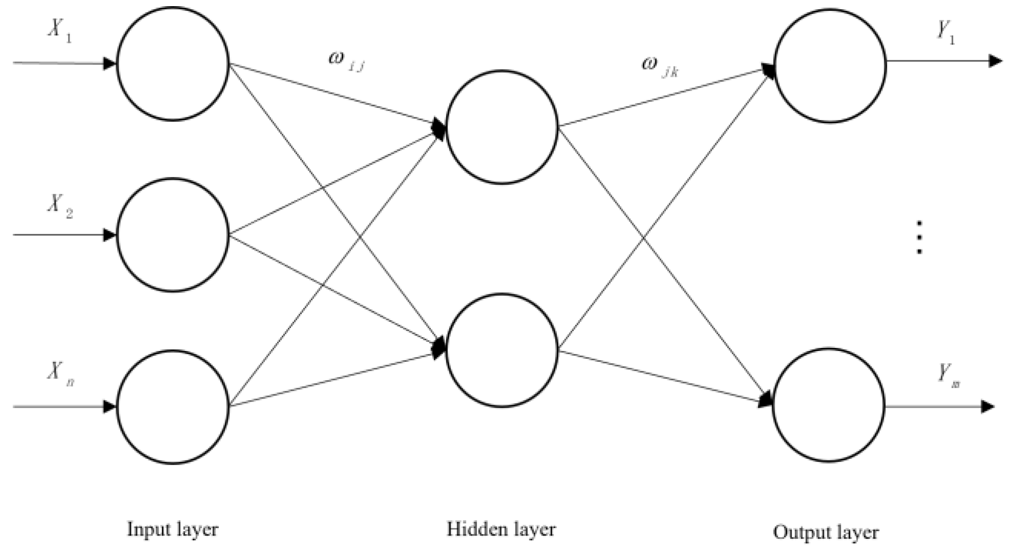
51]. In forward propagation, the input layer is processed layer by layer from the input layer through the hidden layer until the output layer. The state of the neurons in each layer only affects the state of the neurons in the next layer. If the output layer cannot obtain the expected output, it is transferred to the back propagation, and the network weight and threshold are adjusted according to the prediction error so that the predicted output of the BP neural network is constantly approaching the expected output. Setting X1, X2..., Xn as the input values of the BP neural network, Y1, Y2..., Ym are the predicted values of the BP neural network, and Wij and Wjk are the weights of the BP neural network. The BP neural network can be regarded as a nonlinear function. The input and predicted values of the network are the independent and dependent variables of the function, respectively. When the number of input nodes is
n and the number of output nodes is m, the BP neural network expresses the function mapping relationship from
n independent variables to m dependent variables. The topology structure of BP neural network is shown in
Figure 3.
A genetic algorithm is a computational model of the biological evolution process simulating natural selection and the genetic mechanism of Darwinian biological evolution, and it is a method used to search for an optimal solution by simulating the natural evolution process [
52]. It was first proposed by Professor J. Halland from the University of Michigan in the United States. It simulates the phenomena of replication, crossover, and variation occurring in natural selection and heredity. Starting from any initial population, it generates a group of individuals better adapted to the environment through random selection, crossover, and mutation operations. The population is made to evolve to better and better areas in the search space so that there is generation after generation of continuous evolution, and finally a group of individuals most adapted to the environment is converged to in order to obtain the optimal solution to the problem.
Previous studies have shown that in the process of gradient descent optimization, a BP neural network has defects such as slow learning convergence speed, the network structure being difficult to determine, and a local minimum value being easy to fall into in network training, resulting in a decline in application value [
53]. A genetic algorithm is an adaptive global search optimal solution algorithm formed in the process of simulating natural genetic mechanisms and evolution. It has the advantages of parallelism, robustness, and global optimality. It can effectively resolve the risk that the training process of a BP neural network becomes limited to the local optimal and optimize the initial weight and threshold of a BP neural network to improve the stability of the BP neural network [
54]. In this study, GA was combined with a BP neural network, and the initial weight and threshold of the BP neural network were optimized by GA to solve the defects of the BP neural network, such as it being too dependent on experience and having a slow convergence speed, and this was applied to the wettability identification of coal dust.
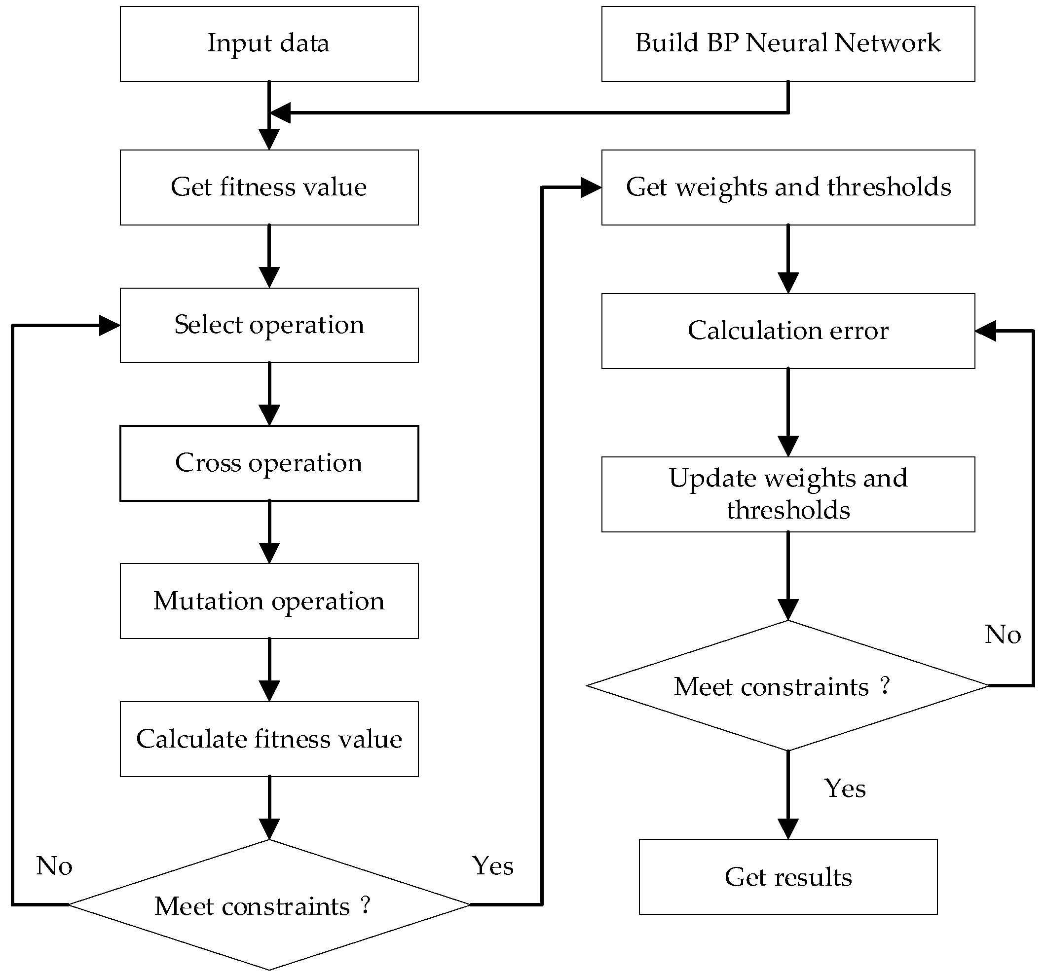
The genetic algorithm optimization of the BP neural network was based on the establishment of a BP neural network structure using a genetic algorithm to optimize the weight and threshold of the neural network, and then the optimized BP neural network was used for analysis and prediction. The training flow chart is shown in
Figure 4.
The process of optimizing the BP neural network based on the genetic algorithm is as follows:
(1) Read data.
(2) Preprocess data as follows:
where
is the lowest value of a data sequence and
is the highest value of the data sequence.
(3) Set the optimal hidden layer node number and select an empirical formula as follows:
where
,
, and
are the numbers of the hidden layer, input layer, and output layer nodes, respectively, and the value of
is typically between 0 and 10.
(4) Perform the initialization, selection, crossover, and mutation of the GA.
The GA used in this study adopted the roulette method for the selection operation, and the selection probability
of individual
is expressed as
where
is the individual fitness,
is the coefficient, and
is the number of individuals in the population.
Real number coding and crossover processing are performed on the individual, and the crossover operation method of the
chromosome,
, and
chromosome,
, at position
is as follows:
where
is a random number in the interval [0, 1].
The mutation operation on gene j of individual
is as follows:
where
is the upper bound of
,
is the lower bound of
,
,
is a random evolutionary number,
is the current number of iterations,
is the maximum number of evolutions, and
is a random number in [0, 1].
(5) Perform real number coding on the population, where the fitness value,
, is the error between the predicted and expected data, expressed as follows:
where
is the number of output nodes of the BP neural network,
is the expected output value of node
of the BP neural network,
is the predicted output value for node
, and
is a coefficient.
(6) Circularly iterate the optimal initial weight value and threshold value.
(7) Construct a BP neural network using the optimal initial weight value and threshold value obtained via circular iteration.
(8) Import training data, input_train, to train a BP neural network.
(9) Transfer the test data, input_test, in the dataset into the trained neural network for testing and perform inverse normalization processing on the prediction data.
(10) Perform an error analysis on the expected and predicted values.
3.2. Establishment of Model
This study was based on the MATLAB R2020a software for experimental research. The training set and testing set were randomly selected, among which thirty sets of training and five sets of testing were used for this model. In the MATLAB neural network toolbox, the newff () function was used to create the BP neural network, the mapminmax () function was used to normalize and de-normalize the data, the train () function was used to train, and the sim () function was used to complete the network simulation. This model was based on the rand () function in MATLAB, which randomly selected thirty samples out of the thirty-five as the training set and the remaining five samples as the test set. The purpose of the training set was to build the model, while the purpose of the validation set was to use each model to record the accuracy of the model in order to find out the model with the best effect. The validation set was automatically generated by newff () function in the MATLAB neural network toolbox to select the parameters corresponding to the model with the best effect, that is, to adjust the model parameters. After obtaining the optimal model through the training set and validation set, the test set was used for the model prediction.
3.2.1. GA–BP Hidden Layer Number Selection
According to Formula (2), the number of hidden layers in this test was between three and fifteen. There was an inverse relationship between the RRMSE value and the model fitting effect, that is, the smaller the RRMSE value, the better the fitting effect. The training process showed that when the number of hidden layer nodes was three, the corresponding root mean square error reached the minimum of 0.016256, so the number of hidden layer nodes in the neural network was determined to be three. The corresponding relationship between the number of hidden layer nodes and the root mean square error is shown in
Table 3.
In this study, 13 influencing factors of coal dust wettability were taken as the input parameters, and the estimated value of the contact angle was taken as the output parameter. Therefore, the input and output parameters of the fitting nonlinear function in the model were thirteen and one, respectively. The structure of the GA–BP model was 13–3–1, namely, there were thirteen nodes in the input layer, three nodes in the hidden layer, and one node in the output layer. There were forty-two common weights (13 × 3 + 3 × 1 = 42) and four threshold values (3 + 1 = 4), so the individual coding length of the neural network was forty-six (42 + 4 = 46).
3.2.2. Parameter Setting of GA–BP Model
Goal represents the minimum error of the training goal; epochs represents the number of training sessions; show represents the display frequency of training iterations; lr represents the learning rate; mc represents the momentum factor; min_grad represents the minimum performance gradient; and max_fail represents the highest number of failures. These were set to 0.00001, 1000, 25, 0.01, 0.01, 10
−6, and 6, respectively, in sequence. The common parameters of the BP neural network and GA–BP, including the minimum error of the training target, training times, learning rate, momentum factor, minimum performance gradient, and maximum failure times, were set as the same. The parameter settings of the GA–BP model are shown in
Table 4, and the diagram of the network training parameters is shown in
Figure 5.


 ,
, 


