
A Survey of the Landscape Visibility Analysis Tools and Technical Improvements
 ,
,
Abstract
:1. Introduction
2. A Review of Approaches to Landscape Visibility Analysis
2.1. Definitions and Generations of Previous Methods
2.2. Technical Comparison
2.3. Strengths and Weaknesses of the Existing Tools
- (1)
- ArcGIS and ArcGIS Pro
- (2)
- Supermap
- (3)
- Depth Space 3D based on Graph Theory’s Depthmap
- (4)
- 3D Isovist of the Grasshopper plug-in DeCodingSpaces and a view analysis of the Grasshopper plug-in Ladybug

| Supported and Related Methods | ESRI Series ArcGIS; GRASSGIS | Supermap | Depth Space 3D | Rhino Grasshopper Plugin DeCodingSpaces | Rhino Grasshopper Plugin Ladybug |
|---|---|---|---|---|---|
| Viewshed [17] | Optimized | Optimized | Simplified | ||
| Isovist [19] | Optimized | Usage | Usage | ||
| VGA [21] | Optimized | Simplified | Optimized | ||
| Voxel [36] | |||||
| Visualscape [22] | Simplified | ||||
| Viewscape [61] | Simplified | ||||
| Viewnets or Line of Sight [57] | Optimized | Optimized | Optimized | ||
| 3D Visibility/Ray Casting [40] | Optimized | Optimized | Optimized | ||
| 3D VGA [44] | Optimized |
| Performance Comparison | ESRI Series ArcGIS; GRASSGIS | Supermap | Depth Space 3D | Rhino Grasshopper Plugin DeCodingSpaces | Rhino Grasshopper Plugin Ladybug |
|---|---|---|---|---|---|
| User Interaction | |||||
| Viewpoint and Analysis Object Selection | Layer selection | Click | Click, Layer selection | Click, Region selection | Click, Region selection |
| Visibility Obstacles | |||||
| Building Obstacles | Good | Good | Good | Good | Good |
| Terrain Obstacles | Good | Good | Good | Good | Good |
| Tree Obstacles | Mediocre | Mediocre | Mediocre | ||
| Data source | |||||
| Building Data | Mediocre | Good | Good | Good | Good |
| Landscape Terrain Data | Good | Good | Good | Mediocre | Good |
| Urban surface Data | Mediocre | Mediocre | Good | Mediocre | Good |
| Open Source | |||||
| API Acquire | Fully opensource | Fully opensource | |||
| Computing Capacity | |||||
| GPU-Based Parallel Processing | Unknown | Usage | Usage | ||
| Parallel Multiple Viewpoints Computing | Mediocre | Mediocre | Good | Mediocre | Good |
| Analysis Object | |||||
| DEM/Raster | Usage | Usage | Usage | Transfer | Transfer |
| Shape/Polygon | Transfer | Transfer | Transfer | Usage | Usage |
| Mesh | Transfer | Usage | Usage | ||
| Brep | Usage | Usage | |||
| Airborne LiDAR | Usage | ||||
| Outcome | |||||
| Visualization | Good | Good | Good | Good | Good |
| Parametric | - | - | - | Measure the list of line of sight | Measure the list of mesh values, measure the distance from VP to the mesh centroid |
| Geometric | Raster | - | Triangular polygon surface | Result Isovist geometry, line of sight | Result triangular Mesh, Mesh centroid |
| User Intervention | Low, Fixed result | Low, Fixed result | Low, Fixed result | Varies with applications | High, Evaluation of outcomes |
| Method Generation | 2–3 *** | 2 ** | 2–3 *** | 2 ** | 3 *** |
3. Visual to Perceptual: Towards Dynamic Landscape Perceptions
3.1. Optimization Route and Conceptual Framework
3.2. Performance Examination Criteria
4. Data and Methods
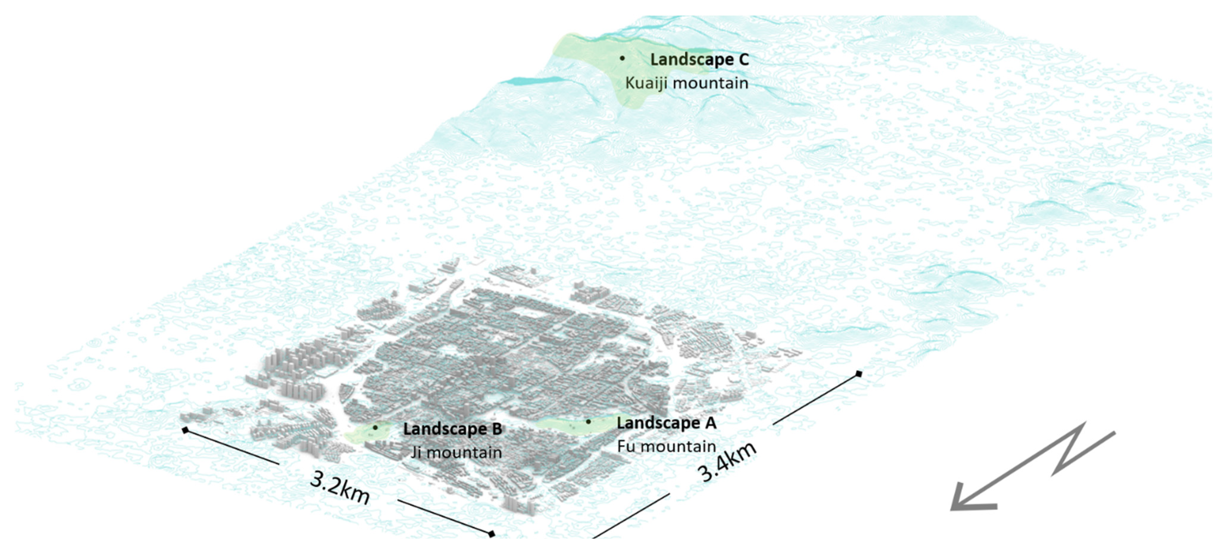
4.1. Study Area
4.2. Data
4.2.1. Spatial Background
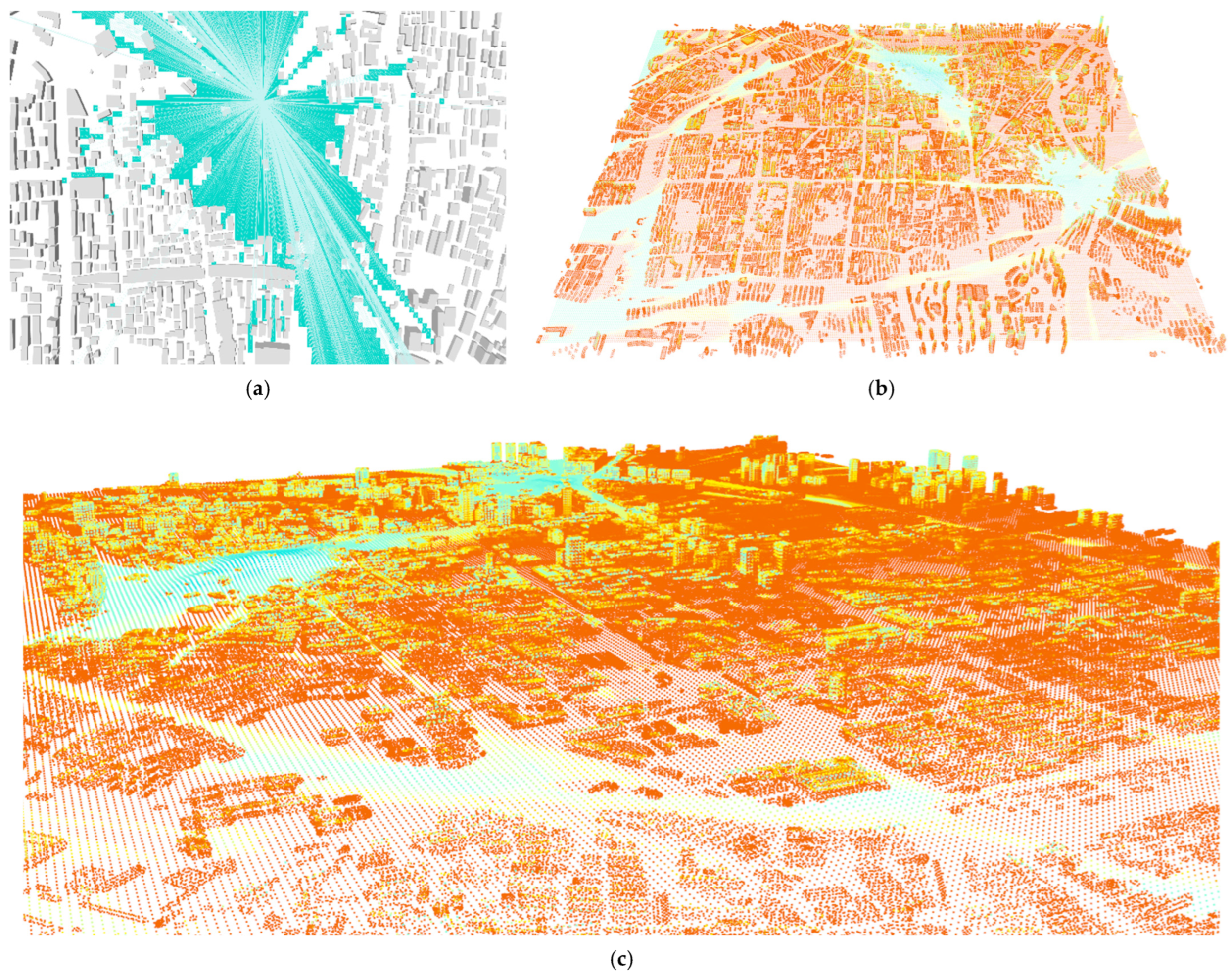
4.2.2. Viewpoint Input Settings
4.2.3. Visibility and Spatial Indices Measurement
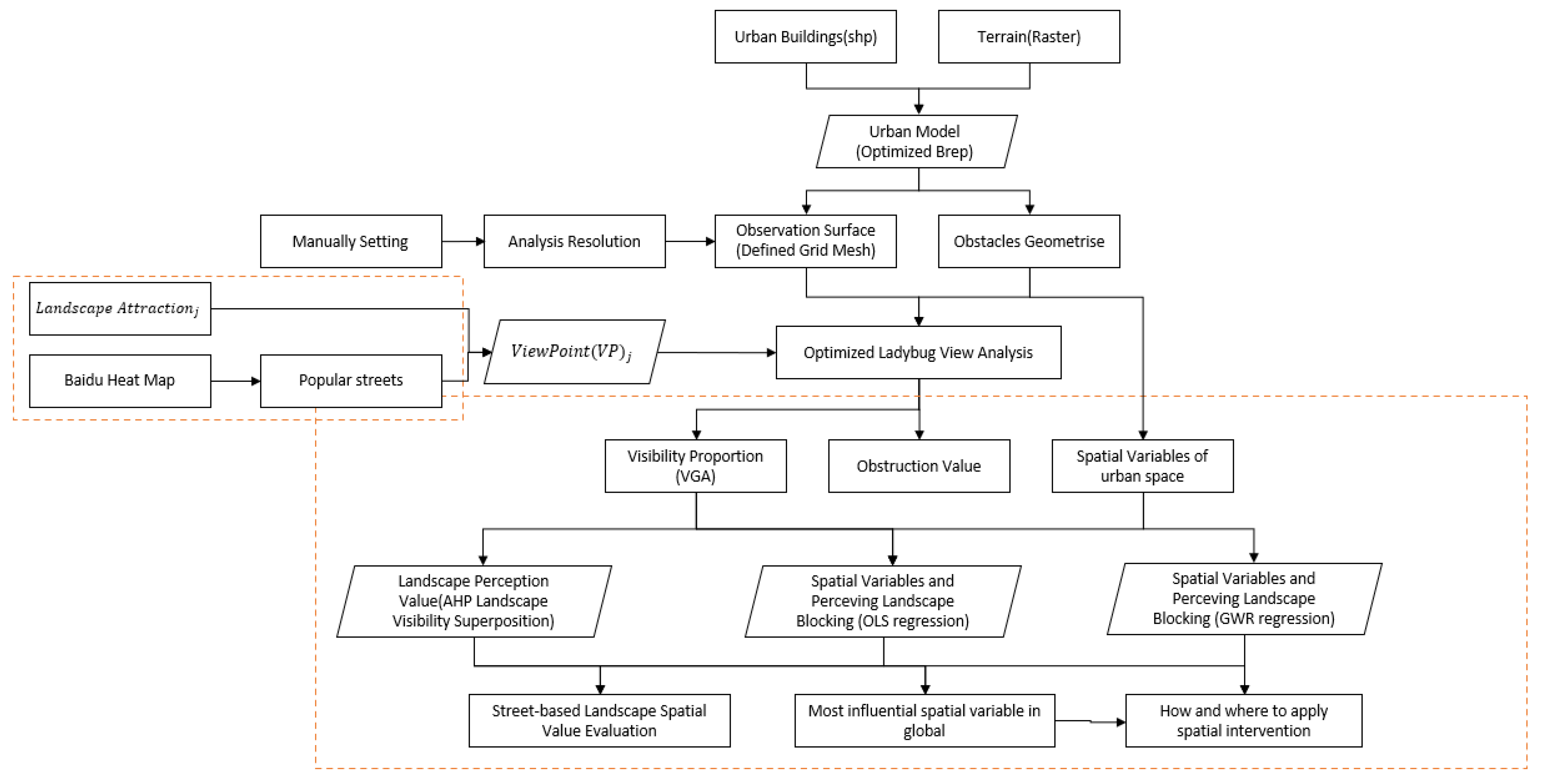
4.3. Visibility-Oriented Interaction Model Architecture
5. Results and Discussions
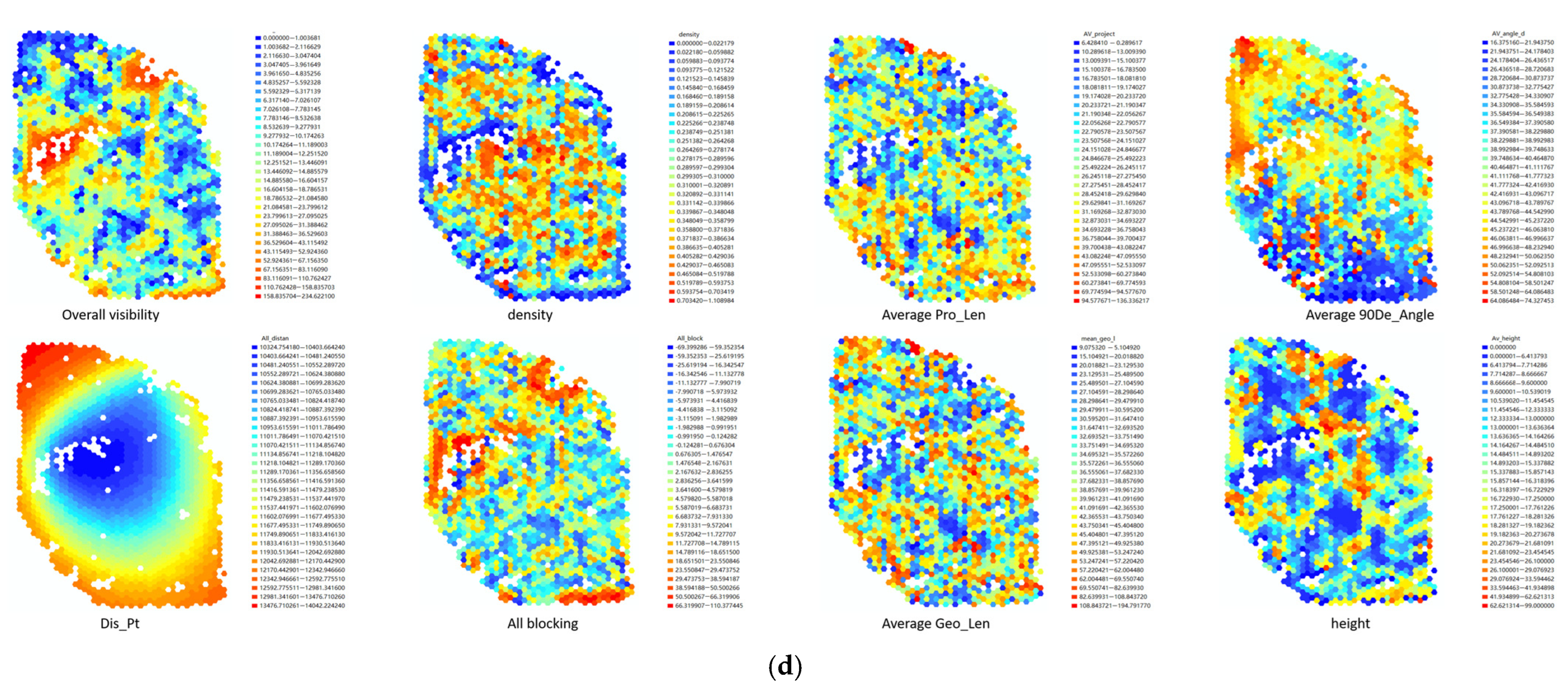
5.1. Landscape Spatial Value Evaluation
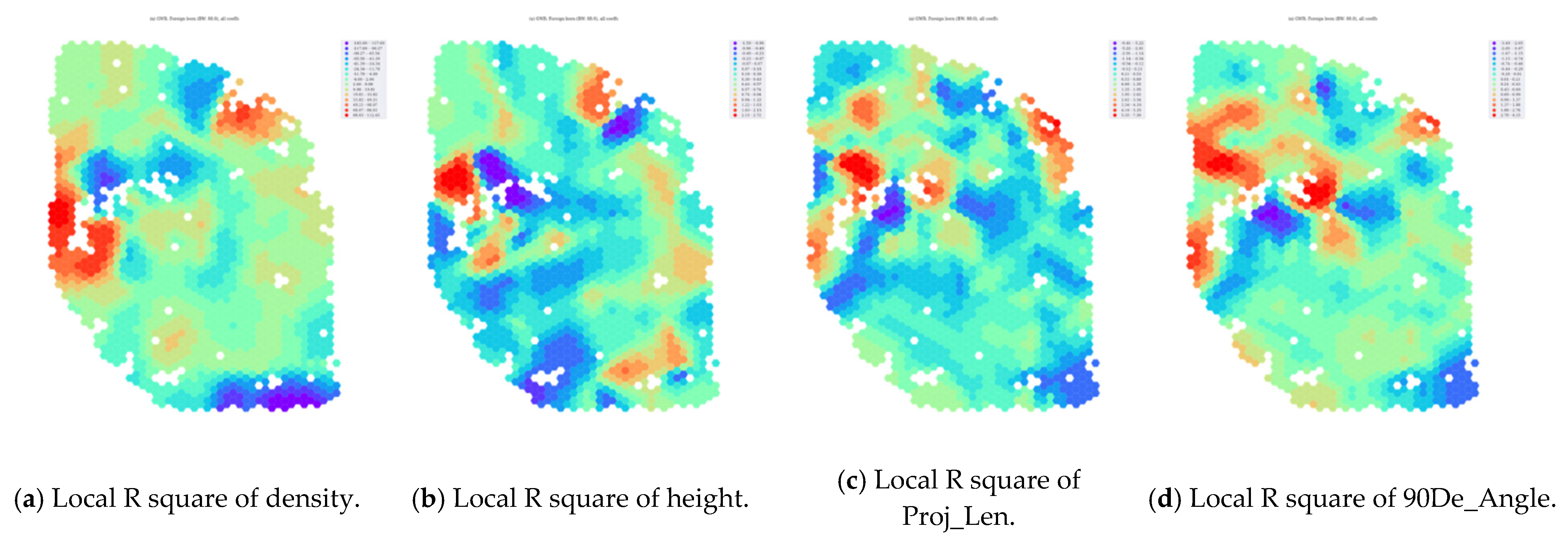
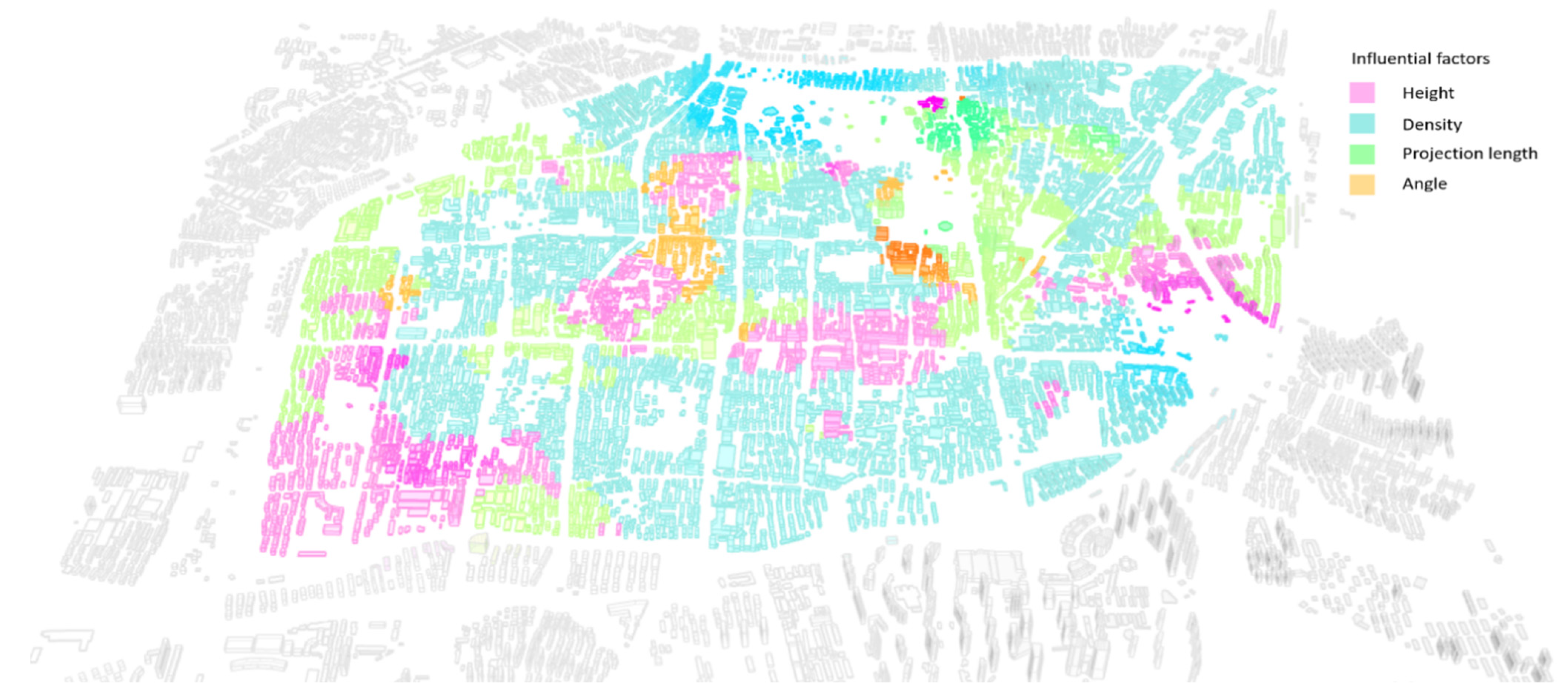
5.2. Influential Obstacles and Interventions
5.3. Test of the Predefined Goals
5.4. Limitations
6. Conclusions
Author Contributions
Funding
Institutional Review Board Statement
Informed Consent Statement
Data Availability Statement
Acknowledgments
Conflicts of Interest
References
- Natapov, A.; Fisher-Gewirtzman, D. Cities as Visuospatial Networks. In Smart City Networks; Rassia, S.T., Pardalos, P.M., Eds.; Springer Optimization and Its Applications; Springer International Publishing: Cham, Switzerland, 2017; Volume 125, pp. 191–205. ISBN 978-3-319-61312-3. [Google Scholar]
- Jacobs, J. The Death and Life of Great American Cities; Vintage Reissue edition (1 December 1992); Vintage: New York, NY, USA; ISBN 978-0-394-42159-9.
- Appleyard, D.; Lynch, K.; Myer, J.R. The View from the Road; MIT Press: Cambridge, MA, USA, 1966. [Google Scholar]
- Lynch, K. The Image of the City, 21st ed.; The MIT Press: Cambridge, MA, USA, 1992; ISBN 978-0-262-62001-7. [Google Scholar]
- O’Sullivan, D.; Turner, A. Visibility graphs and landscape visibility analysis. Int. J. Geogr. Inf. Sci. 2001, 15, 221–237. [Google Scholar] [CrossRef]
- Ewing, R.; Handy, S. Measuring the Unmeasurable: Urban Design Qualities Related to Walkability. J. Urban Des. 2009, 14, 65–84. [Google Scholar] [CrossRef]
- Lynch, K. Managing the Sense of a Region; MIT Press: Cambridge, MA, USA, 1976; ISBN 978-0-262-12072-2. [Google Scholar]
- Hillier, B.; Penn, A.; Hanson, J.; Grajewski, T.; Xu, J. Natural movement: Or, configuration and attraction in urban pedestrian movement. Environ. Plan. B Plan. Des. 1993, 20, 29–66. [Google Scholar] [CrossRef] [Green Version]
- Hillier, B.; Iida, S. Network and Psychological Effects in Urban Movement. In Spatial Information Theory; Cohn, A.G., Mark, D.M., Eds.; Lecture Notes in Computer Science; Springer: Berlin/Heidelberg, Germany, 2005; Volume 3693, pp. 475–490. ISBN 978-3-540-28964-7. [Google Scholar]
- Wu, Z.; Feng, F.; Lu, F.; Yang, T.; Gan, W. Space Design for Urban Resilience. Time Archit. 2020, 84–89. [Google Scholar] [CrossRef]
- Kandel, E.R.; Schwartz, J.H.; Jessell, T.M.; Siegelbaum, S.A.; Hudspeth, A.J. Principles of Neural Science, 5th ed.; McGraw Hill Professional: New York, NY, USA, 2012; ISBN 978-0-07-181001-2. [Google Scholar]
- Inglis, N.C.; Vukomanovic, J.; Costanza, J.; Singh, K.K. From viewsheds to viewscapes: Trends in landscape visibility and visual quality research. Landsc. Urban Plan. 2022, 224, 104424. [Google Scholar] [CrossRef]
- Batty, M.; Torrens, P.M. Modelling complexity: The limits to prediction. Cybergeo 2001. [Google Scholar] [CrossRef]
- Goodman, D.; Goodman, M.K. Alternative Food Networks. In International Encyclopedia of Human Geography; Kitchin, R., Thrift, N., Eds.; Elsevier: Oxford, UK, 2009; Volume 4, pp. 208–220. ISBN 978-0-08-044910-4. [Google Scholar]
- Zhang, J.; Li, Q. Research on the Complex Mechanism of Placeness, Sense of Place, and Satisfaction of Historical and Cultural Blocks in Beijing’s Old City Based on Structural Equation Model. Complexity 2021, 2021, 6673158. [Google Scholar] [CrossRef]
- Kang, N.; Liu, C. Towards landscape visual quality evaluation: Methodologies, technologies, and recommendations. Ecol. Indic. 2022, 142, 109174. [Google Scholar] [CrossRef]
- Tandy, C.R.V. The Isovist Method of Landscape Survey. Methods Landsc. Anal. 1967, 10, 9–10. [Google Scholar]
- Amidon, E.L.; Elsner, G.H. Delineating Landscape View Areas… A Computer Approach; Res Note PSW-RN-180; U.S. Department of Agriculture, Forest Service, Pacific Southwest Forest and Range Experiment Station: Berkeley, CA, USA, 1968; 5p.
- Benedikt, M.L. To take hold of space: Isovists and isovist fields. Environ. Plan. B Plan. Des. 1979, 6, 47–65. [Google Scholar] [CrossRef]
- Batty, M. Exploring Isovist Fields: Space and Shape in Architectural and Urban Morphology. Environ. Plan. B Plan. Des. 2001, 28, 123–150. [Google Scholar] [CrossRef]
- Turner, A.; Doxa, M.; O’Sullivan, D.; Penn, A. From Isovists to Visibility Graphs: A Methodology for the Analysis of Architectural Space. Environ. Plan. B Plan. Des. 2001, 28, 103–121. [Google Scholar] [CrossRef] [Green Version]
- Llobera, M. Extending GIS-based visual analysis: The concept of visualscapes. Int. J. Geogr. Inf. Sci. 2003, 17, 25–48. [Google Scholar] [CrossRef]
- Fisher-Gewirtzman, D.; Burt, M.; Tzamir, Y. A 3-D Visual Method for Comparative Evaluation of Dense Built-up Environments. Environ. Plan. B Plan. Des. 2003, 30, 575–587. [Google Scholar] [CrossRef] [Green Version]
- Yang, P.P.-J.; Putra, S.Y.; Li, W. Viewsphere: A GIS-based 3D visibility analysis for urban design evaluation. Environ. Plan. B Plan. Des. 2007, 34, 971–992. [Google Scholar] [CrossRef] [Green Version]
- Chmielewski, S.; Tompalski, P. Estimating outdoor advertising media visibility with voxel-based approach. Appl. Geogr. 2017, 87, 1–13. [Google Scholar] [CrossRef]
- Michael, R. Travis, VIEWIT: Computation of Seen Areas, Slope, and Aspect for Land-Use Planning; Pacific Southwest Forest and Range Experiment Station; Pacific Southwest Research Station, Forest Service, U.S. Department of Agriculture: Berkeley, CA, USA, 1975; 70p.
- Felleman, J.P. Landscape Visibility Mapping: Theory and Practice; State University of New: New York, NY, USA, 1979; p. 125. [Google Scholar]
- Van den Berg, A.; Van Lith, J.; Roos, J. Toepassing van het computerprogramma MAP2 in het landschapsbouwkundig onderzoek. Landschap 1985, 2, 278–293. [Google Scholar]
- Fisher, P.F. First Experiments in Viewshed Uncertainty: Simulating Fuzzy Viewsheds. Photogramm. Photogramm. Eng. Remote Sens. 1992, 58, 345–352. [Google Scholar]
- Fisher, P. Probable and Fuzzy Models of the Viewshed Operation. In Innovations in GIS; Worboys, M., Ed.; Taylor & Francis: Abingdon, UK, 1994; pp. 161–175. [Google Scholar]
- Ogburn, D.E. Assessing the level of visibility of cultural objects in past landscapes. J. Archaeol. Sci. 2006, 33, 405–413. [Google Scholar] [CrossRef]
- Pyysalo, U.; Oksanen, J.; Sarjakoski, T. Viewshed analysis and visualization of landscape voxel models. In Proceedings of the 24th International Cartographic Conference, Santiago, Chile, 15–21 November 2009; p. 11. [Google Scholar]
- Hagstrom, S.; Messinger, D. Line-of-sight analysis using voxelized discrete lidar. In Proceedings of the Laser Radar Technology and Applications XVI, Orlando, FL, USA, 27–29 April 2011; Turner, M.D., Kamerman, G.W., Eds.; pp. 80370B–80370B-11. [Google Scholar] [CrossRef]
- Morello, E.; Ratti, C. A digital image of the city: 3D isovists in Lynch’s urban analysis. Environ. Plan. B Plan. Des. 2009, 36, 837–853. [Google Scholar] [CrossRef] [Green Version]
- Fishergewirtzman, D. 3D Models as a Platform for Urban Analysis and Studies on Human Perception of Space. Usage Usability Util. 3D City Model. 2012, 01001. [Google Scholar] [CrossRef] [Green Version]
- Fisher-Gewirtzman, D.; Shashkov, A.; Doytsher, Y. Voxel based volumetric visibility analysis of urban environments. Surv. Rev. 2013, 45, 451–461. [Google Scholar] [CrossRef]
- Chmielewski, S. Towards Managing Visual Pollution: A 3D Isovist and Voxel Approach to Advertisement Billboard Visual Impact Assessment. ISPRS Int. J. Geo-Inform. 2021, 10, 656. [Google Scholar] [CrossRef]
- Kim, G.; Kim, A.; Kim, Y. A new 3D space syntax metric based on 3D isovist capture in urban space using remote sensing technology. Comput. Environ. Urban Syst. 2019, 74, 74–87. [Google Scholar] [CrossRef]
- Zhao, Y.; Wu, B.; Wu, J.; Shu, S.; Liang, H.; Liu, M.; Badenko, V.; Fedotov, A.; Yao, S.; Yu, B. Mapping 3D visibility in an urban street environment from mobile LiDAR point clouds. GISci. Remote Sens. 2020, 57, 797–812. [Google Scholar] [CrossRef]
- Koltsova, A.; Tuncer, B.; Schmitt, G. Visibility Analysis for 3D Urban Environments. In Proceedings of the 31st International Conference on Education and Research in Computer Aided Architectural Design in Europe (ECAADe), Delft, The Netherlands, 18–20 September 2013; Volume 2. [Google Scholar]
- Suleiman, W.; Joliveau, T.; Favier, E. A New Algorithm for 3D Isovist. In Proceedings of the 15th International Symposium on Spatial Data Handling Geospatial Dynamics, Geosimulation and Exploratory Visualization, Bonn, Germany, 22–24 August 2012; pp. 157–173. [Google Scholar]
- Feng, W.; Gang, W.; Deji, P.; Yuan, L.; Liuzhong, Y.; Hongbo, W. A parallel algorithm for viewshed analysis in three-dimensional Digital Earth. Comput. Geosci. 2015, 75, 57–65. [Google Scholar] [CrossRef]
- Chang, D.; Park, J. Quantifying the Visual Experience of Three-dimensional Built Environments. J. Asian Arch. Build. Eng. 2018, 17, 117–124. [Google Scholar] [CrossRef] [Green Version]
- Varoudis, T.; Swenson, A.G.; Kirkton, S.D.; Waters, J.S. Exploring nest structures of acorn dwelling ants with X-ray microtomography and surface-based three-dimensional visibility graph analysis. Philos. Trans. R. Soc. B Biol. Sci. 2018, 373, 20170237. [Google Scholar] [CrossRef] [Green Version]
- Morais, F.; Vaz, J.; Viana, D.; Carvalho, I.C.; Ruivo, C.; Paixão, C.; Tejada, A.; Gomes, T. 3D Space Syntax Analysis—Case Study “Casa Da Música”. In Proceedings of the 11th Space Syntax Symposium, Lisbon, Portugal, 3–7 July 2017. [Google Scholar]
- Ascensão, A.; Costa, L.; Fernandes, C.; Morais, F.; Ruivo, C. 3D Space Syntax Analysis: Attributes to Be Applied in Landscape Architecture Projects. Urban Sci. 2019, 3, 20. [Google Scholar] [CrossRef] [Green Version]
- Domingo-Santos, J.M.; de Villarán, R.F.; Rapp-Arrarás, R.F.; de Provens, E.C.-P. The visual exposure in forest and rural landscapes: An algorithm and a GIS tool. Landsc. Urban Plan. 2011, 101, 52–58. [Google Scholar] [CrossRef]
- Leduc, T.; Kontovourkis, O. Towards a Mixed Approach Combining Visibility and Mobility Studies to Analyze the Eleftheria Square; Societa Editrice Esculapio: Nicosia, Cyprus, 2012; pp. 67–77. ISBN 978-88-7488-546-6. [Google Scholar]
- Fisher-Gewirtzman, D. Integrating ‘weighted views’ to quantitative 3D visibility analysis as a predictive tool for perception of space. Environ. Plan. B Urban Anal. City Sci. 2018, 45, 345–366. [Google Scholar] [CrossRef]
- Putra, S.Y.; Yang, P. Analysing Mental Geography of Residential Environment in Singapore Using GIS-Based 3D Visibility Analysis. In Proceedings of the International Conference ‘Doing, Thinking, Feeling Home: The Mental Geography of Residential Environments’, Delft, The Netherlands, 14–15 October 2005. [Google Scholar]
- Tara, A.; Belesky, P.; Ninsalam, Y. Towards Managing Visual Impacts on Public Spaces: A Quantitative Approach to Studying Visual Complexity and Enclosure Using Visual Bowl and Fractal Dimension. J. Digit. Landsc. Archit. 2019, 4, 21–32. [Google Scholar] [CrossRef]
- Cervilla, A.R.; Tabik, S.; Vías, J.; Mérida, M.; Romero, L.F. Total 3D-viewshed Map: Quantifying the Visible Volume in Digital Elevation Models. Trans. GIS 2016, 21, 591–607. [Google Scholar] [CrossRef]
- Burrough, P.A. Principles of geographical information systems for land resources assessment. Geocarto Int. 1986, 1, 54. [Google Scholar] [CrossRef]
- Ruzickova, K.; Ruzicka, J.; Bitta, J. A new GIS-compatible methodology for visibility analysis in digital surface models of earth sites. Geosci. Front. 2021, 12, 101109. [Google Scholar] [CrossRef]
- Stucky, J.L.D. On applying viewshed analysis for determining least-cost paths on Digital Elevation Models. Int. J. Geogr. Inf. Sci. 1998, 12, 891–905. [Google Scholar] [CrossRef]
- Kim, Y.-H.; Rana, S.; Wise, S. Exploring multiple viewshed analysis using terrain features and optimisation techniques. Comput. Geosci. 2004, 30, 1019–1032. [Google Scholar] [CrossRef] [Green Version]
- Van Dyke, R.M.; Bocinsky, R.K.; Windes, T.C.; Robinson, T.J. Great Houses, Shrines, and High Places: Intervisibility in the Chacoan World. Am. Antiq. 2016, 81, 205–230. [Google Scholar] [CrossRef] [Green Version]
- Li, H.; Yang, M.; Kim, J.H.; Zhang, C.; Liu, R.; Huang, P.; Liang, D.; Zhang, X.; Li, X.; Ying, L. SuperMAP: Deep ultrafast MR relaxometry with joint spatiotemporal undersampling. Magn. Reson. Med. 2023, 89, 64–76. [Google Scholar] [CrossRef]
- Koenig, R.; Miao, Y.; Aichinger, A.; Knecht, K.; Konieva, K. Integrating urban analysis, generative design, and evolutionary optimization for solving urban design problems. Environ. Plan. B Urban Anal. City Sci. 2020, 47, 997–1013. [Google Scholar] [CrossRef]
- Koenig, R.; Miao, Y.; Schneider, S.; Vesely, O.; Buš, P.; Bielik, M.; Abdulmawla, A.; Dennemark, M.; Fuchkina, E.; Aichinger, A.; et al. DeCodingSpaces Toolbox for Grasshopper: Computational Analysis and Generation of STREET NETWORK, PLOTS and BUILDINGS; Computational Planning Group (CPlan) Software Package, Internet Webpage. Available online: http://decodingspaces-toolbox.org/ (accessed on 17 July 2019).
- Vukomanovic, J.; Singh, K.K.; Petrasova, A.; Vogler, J.B. Not seeing the forest for the trees: Modeling exurban viewscapes with LiDAR. Landsc. Urban Plan. 2018, 170, 169–176. [Google Scholar] [CrossRef]
- Puspitasari, A.W.; Kwon, J. Comparison of Spatial Layout of Tall Buildings Clustered in Circular, Rectangular, and Linear Geographical Areas and Impact on Skyline. Buildings 2020, 10, 64. [Google Scholar] [CrossRef]
- Yin, L. Street level urban design qualities for walkability: Combining 2D and 3D GIS measures. Comput. Environ. Urban Syst. 2017, 64, 288–296. [Google Scholar] [CrossRef]
- Shen, Y.; Zhuo, J.; Wu, Z. Precise Urban Design-Toward Socially Sustainable Urban Form. Time Archit. 2021, 26–33. [Google Scholar] [CrossRef]
- Wu, Z.; Qiao, R.; Zhao, S.; Liu, X.; Gao, S.; Liu, Z.; Ao, X.; Zhou, S.; Wang, Z.; Jiang, Q. Nonlinear forces in urban thermal environment using Bayesian optimization-based ensemble learning. Sci. Total Environ. 2022, 838, 156348. [Google Scholar] [CrossRef]
- Turner, M.G.; Gardner, R.H.; O’Neill, R.V. Landscape Ecology in Theory and Practice: Pattern and Process; Springer: New York, NY, USA, 2001; ISBN 978-0-387-95122-5. [Google Scholar]
- Meentemeyer, R.K.; Haas, S.E.; Václavík, T. Landscape Epidemiology of Emerging Infectious Diseases in Natural and Human-Altered Ecosystems. Annu. Rev. Phytopathol. 2012, 50, 379–402. [Google Scholar] [CrossRef] [Green Version]
- Dai, L.; Derudder, B.; Liu, X.; Ye, L.; Duan, X. Simulating infrastructure networks in the Yangtze River Delta (China) using generative urban network models. Belgeo 2016. [Google Scholar] [CrossRef] [Green Version]
- Porfyriou, H. Urban Heritage Conservation of China’s Historic Water Towns and the Role of Professor Ruan Yisan: Nanxun, Tongli, and Wuzhen. Heritage 2019, 2, 149. [Google Scholar] [CrossRef] [Green Version]
- Wu, Z. Five Current Themes of Protection and Renewal of Famous Cities. China Anc. City 2022, 36, 1–2. [Google Scholar] [CrossRef]
- Zhou, S.; Liu, Z.; Wang, M.; Gan, W.; Zhao, Z.; Wu, Z. Impacts of building configurations on urban stormwater management at a block scale using XGBoost. Sustain. Cities Soc. 2022, 87, 104235. [Google Scholar] [CrossRef]
- Shaoxing Celebrates Third Ancient City Protection Day. Available online: http://www.ezhejiang.gov.cn/shaoxing/2021-07/19/c_667127.htm (accessed on 23 November 2022).
- Historical City Creates Low Skyline to Highlight Cultural Heritage. Available online: http://www.ezhejiang.gov.cn/shaoxing/2021-02/02/c_586821.htm (accessed on 23 November 2022).

| Visibility Method | Authors | 2D or 3D | Measuring the Visible Building Surface | Measuring the Volume of Obstacles | Responsiveness of Analysis–Design Interaction | Superposition of Multiple Analysis Objects | Embodiment of Complex Urban Saturations in the Case Test |
|---|---|---|---|---|---|---|---|
| 2D Visibility | Amidon and Elsner [18]; Travis et al. [26] | 2D | No | No | No | No | No |
| 2D Isovist | Tandy [17]; Benedikt [19]; Batty [20]; Turner et al. [21] | 2D | No | No | No | No | No |
| 2D VGA | O’Sullivan and Turner [5]; Turner et al. [21] | 2D | No | No | No | Not Tested | No |
| 2D Viewshed | Felleman [27]; Van den Berg, Van Lith, and Roos [28] | 2D | No | No | No | No | No |
| Fuzzy and Cumulative Viewshed | Fisher [29,30]; Ogburn [31] | 2D | No | No | No | Not Tested | No |
| Visualscape | Llobera [22] | 2D | No | No | No | Not Tested | No |
| Viewsphere | Yang, Putra, and Li [24] | 3D | No | No | No | Not Tested | No |
| Viewshed on Voxel model | Pyysalo, Oksanen, and Sarjakoski [32] | 3D | No | No | No | No | No |
| LoSe and Voxelized Scene | Hagstrom and Messinger [33] | 3D | Not Tested | No | No | Not Tested | No |
| 3D Isovist | Morello and Ratti [34] | 3D | Not Tested | No | No | Not Tested | Yes |
| 3D Isovist—Advanced Spatial Openness Index | Fisher-Gewirtzman [35,36] | 3D | Yes | No | Not Tested | Not Tested | No |
| 3D Isovist (Voxel Method) | Chmielewski [37] | 3D | Yes | Not Tested | Not Tested | Not Tested | No |
| 3D Isovist—Optimized by Remote Sensing and LiDAR | Kim, Kim, and Kim [38]; Zhao et al. [39] | 3D | Yes | No | Not Tested | Not Tested | No |
| 3D Visibility (Ray Casting) | Koltsova, Tuncer, and Schmitt [40] | 3D | Yes | No | Not Tested | Not Tested | No |
| 3D Vector Visibility | Suleiman, Joliveau, and Favier [41] | 3D | Yes | No | Not Tested | Not Tested | No |
| 3D Viewshed (Vertex Shader) | Feng et al. [42] | 3D | Yes | No | Not Tested | No | No |
| 3D Visibility (Voxel Method) | Chmielewski and Tompalski [25] | 3D | Yes | Not Tested | Not Tested | Not Tested | No |
| 3D Visibility (with Visual Experience) | Chang and Park [43] | 3D | Yes | No | Not Tested | Not Tested | Yes |
| 3D VGA | Varoudis et al. [44] | 3D | Yes | No | Not Tested | Not Tested | No |
| 3D Space Syntax | Morais et al. [45]; Ascensão et al. [46] | 3D | Not Tested | No | Not Tested | Not Tested | Yes |
| Typical Research | Tools/Software | Input Data Categories | Analysis Resolution Space | Study Object Types | Study Area | Basic Evaluation Rules | Validation |
|---|---|---|---|---|---|---|---|
| Morais et al. [45] | Depth Space 3D | Buildings, Landform | 10 m | Measured all buildings and ground surfaces | Casa da Música, approximately 0.8 km2 | Using the visualization to show the different kinds of space densities | Open CV to trace space dynamic |
| Ascensão et al. [46] | Depth Space 3D | Buildings, Landforms, Vegetation | Not mentioned | Measured all buildings, trees, and ground surfaces | Maia Park, approximately 0.2 km2 | Percentage of the visible pixels of the total pixels; seasonal changes in vegetation on visibility | - |
| Morello and Ratti [34] | 3D Isovist, Optimized in ArcGIS | Buildings | Not mentioned | Measured all building geometries | Milan Trade Fair, 1 km2 | Using the line-of-sight method to evaluate Kevin Lynch’s 5 attributes through movement | - |
| Suleiman, Joliveau, and Favier [41] | ArcGIS and MATLAB | Buildings | Not mentioned | Measured the visibility of the building facade from a vantage point | 500 m radius area | Compute more open space indices in a 3D environment, such as openness, enclosure, and scale | Compared with the images of the 3D environment |
| Rodriguez Cervilla et al. [52] | ArcGIS | Landform | 10 m | Measured the 3D viewshed of terrain from a vantage point | The coastal area of the city of Malaga, 400 km2 | to quantify the Visible volume for a large number of observers in a digital elevation model | - |
| Yin [63] | ArcGIS and ArcScene | Buildings | Not mentioned | Line-of-sight analysis for the building skyline | Downtown Buffalo, 1 m long street | Measure the street-level urban design qualities | - |
| Chmielewski and Tompalski [25] | Voxel-based method | Buildings, Trees, and Terrain | 10 m | Measured the visibility with voxels box through a large number of observation points | 8.8 ha area | Measure the volume of the voxel box to optimize the location of the OA board | - |
| Chmielewski [37] | Voxel-based 3D Isovist method and ArcGIS pro | Buildings, Trees, and Terrain | 0.25 m | Measured the volume of the voxel bounding box (i.e., 3D VGA), the shading of trees was also taken into account | Lublin City (Poland), 1 km radius area | Measure the volume of the voxel bounding box to evaluate the landscape openness | - |
| Koltsova, Tuncer, and Schmitt [40] | Grasshopper, Ray casting method | Buildings, Terrain, Road network | Not mentioned | Measured the visibility of the building facade | Not mentioned, two street block | Combined visibility and accessibility to analyze the visual change through movement | - |
| Tara, Belesky, and Ninsalam [51] | ArcGIS, Grasshopper | Buildings | 4–90 m | Line-of-sight analysis for the building skyline and measured the height and distance of the sight | Unlimited public locations in Melbourne | Measure the urban quality through the sky ratio and fractal dimension | - |
| Puspitasari and Kwon [62] | Grasshopper Ladybug | Buildings, Landform | 5 m | Only studied tower blocks with a height higher than 100 m | 1–4 km2 (1.7 km2 in Lujiazui District) | Percentage of the visible surface area | - |
| Indices | Mathematical Expressions | Diagram | Indices | Mathematical Expressions | Diagram |
|---|---|---|---|---|---|
| 1 Density | The density of buildings within a 100 m radius of the selected building unit |  | 4 Angle deviation with 90 (90De_Angle) | 90 degrees minus the angle between the long side of each building form’s envelope rectangle and the view direction |  |
| 2 Height | The relative height of the building unit above ground level |  | 5 Geometries projection length (Proj_Len) | The actual projection length of the long side of the building’s envelope rectangle relative to the viewpoint |  |
| 3 Geometries length (Geo_Len) | The perimeter of the base of each building unit | 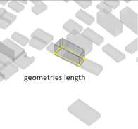 | 6 Distance from landscape focus point (Dis_Pt) | The linear distance of each building to the landscape focus point |  |
| 7 Visibility | The visible score on its surface, and the calculation was computed using Ladybug Grasshopper | 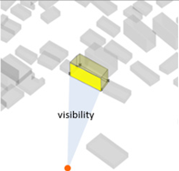 | 8 Visibility blocking | Detected the visibility interference of this building to the buildings behind its surrounding view direction [43] | 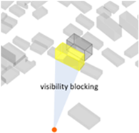 |
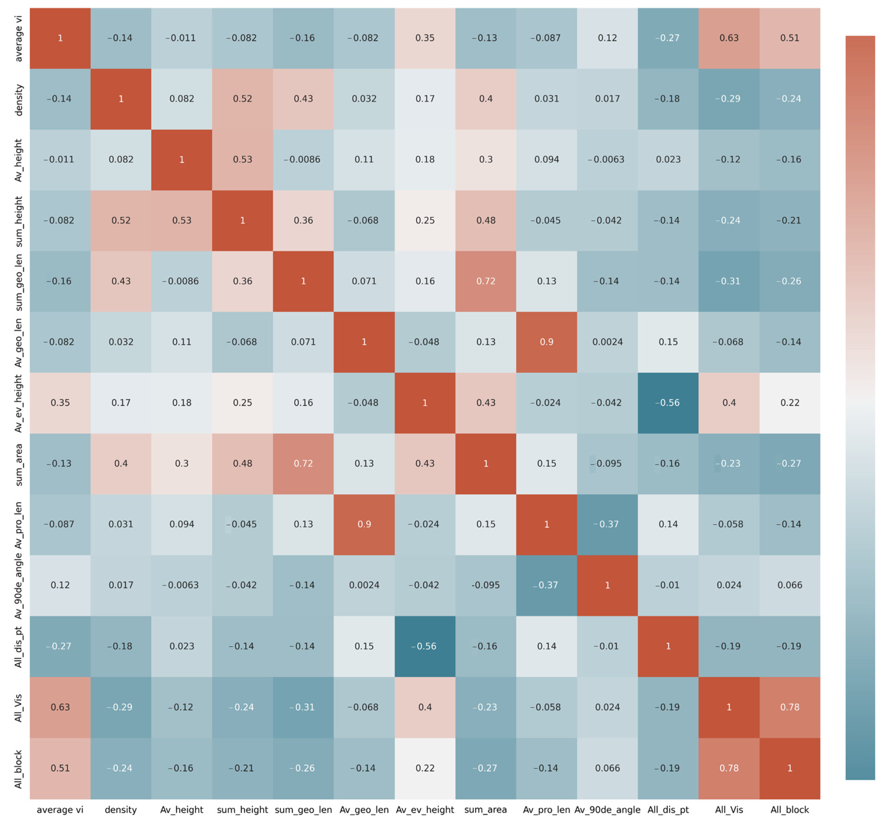
| Variable | VIF | |
|---|---|---|
| 0 | density | 8.026 |
| 1 | Av_height | 6.884 |
| 2 | sum_height | 8.098 |
| 3 | sum_area | 9.961 |
| 4 | Av_ev_height | 16.627 |
| 5 | Av_pro_len | 4.775 |
| 6 | Av_90de_angle | 7.04 |
| 7 | All_dis_pt | 4.071 |
| 8 | All_Vis | 6.856 |
| 9 | All_block | 3.032 |
| Variable | coef | SE | t | p-Value | 0.025 | 0.975 |
|---|---|---|---|---|---|---|
| Density | −21.185 | 2.914 | −7.269 | 0.000 *** | −26.902 | −15.467 |
| Height | 0.338 | 0.055 | 6.185 | 0.000 *** | 0.230 | 0.445 |
| Proj_Len | 0.737 | 0.173 | 4.259 | 0.000 *** | 0.397 | 1.076 |
| 90De_Angle | 0.283 | 0.100 | 2.842 | 0.000 *** | 0.088 | 0.479 |
| OLS Method | GWR Method | ||||||||
|---|---|---|---|---|---|---|---|---|---|
| Variable | Est. | SE | t (Est/SE) | p-Value | Mean | STD | Min. | Median | Max. |
| Density | −20.602 | 2.635 | 7.819 | 0.000 | 0.419 | 30.793 | −145.002 | 3.181 | 112.448 |
| Height | 0.263 | 0.049 | 5.360 | 0.000 | 0.280 | 0.448 | −1.591 | 0.238 | 2.725 |
| Proj_Len | 0.736 | 0.150 | 4.915 | 0.000 | 0.499 | 1.273 | −6.411 | 0.328 | 7.297 |
| 90De_Angle | 0.310 | 0.088 | 3.521 | 0.000 | 0.166 | 0.741 | −3.485 | 0.117 | 4.150 |
Disclaimer/Publisher’s Note: The statements, opinions and data contained in all publications are solely those of the individual author(s) and contributor(s) and not of MDPI and/or the editor(s). MDPI and/or the editor(s) disclaim responsibility for any injury to people or property resulting from any ideas, methods, instructions or products referred to in the content. |
© 2023 by the authors. Licensee MDPI, Basel, Switzerland. This article is an open access article distributed under the terms and conditions of the Creative Commons Attribution (CC BY) license (https://creativecommons.org/licenses/by/4.0/).
Share and Cite
Wu, Z.; Wang, Y.; Gan, W.; Zou, Y.; Dong, W.; Zhou, S.; Wang, M. A Survey of the Landscape Visibility Analysis Tools and Technical Improvements. Int. J. Environ. Res. Public Health 2023, 20, 1788. https://doi.org/10.3390/ijerph20031788
Wu Z, Wang Y, Gan W, Zou Y, Dong W, Zhou S, Wang M. A Survey of the Landscape Visibility Analysis Tools and Technical Improvements. International Journal of Environmental Research and Public Health. 2023; 20(3):1788. https://doi.org/10.3390/ijerph20031788
Chicago/Turabian StyleWu, Zhiqiang, Yuankai Wang, Wei Gan, Yixuan Zou, Wen Dong, Shiqi Zhou, and Mo Wang. 2023. "A Survey of the Landscape Visibility Analysis Tools and Technical Improvements" International Journal of Environmental Research and Public Health 20, no. 3: 1788. https://doi.org/10.3390/ijerph20031788