
Developing a Prediction Model of Demolition-Waste Generation-Rate via Principal Component Analysis


Abstract
:1. Introduction
2. Methods and Materials
2.1. Data Collection and Preprocessing
2.2. Applied Machine-Learning Algorithms
2.2.1. Principal Component Analysis
2.2.2. Linear Regression
2.2.3. K-Nearest Neighbor
2.2.4. Decision Tree
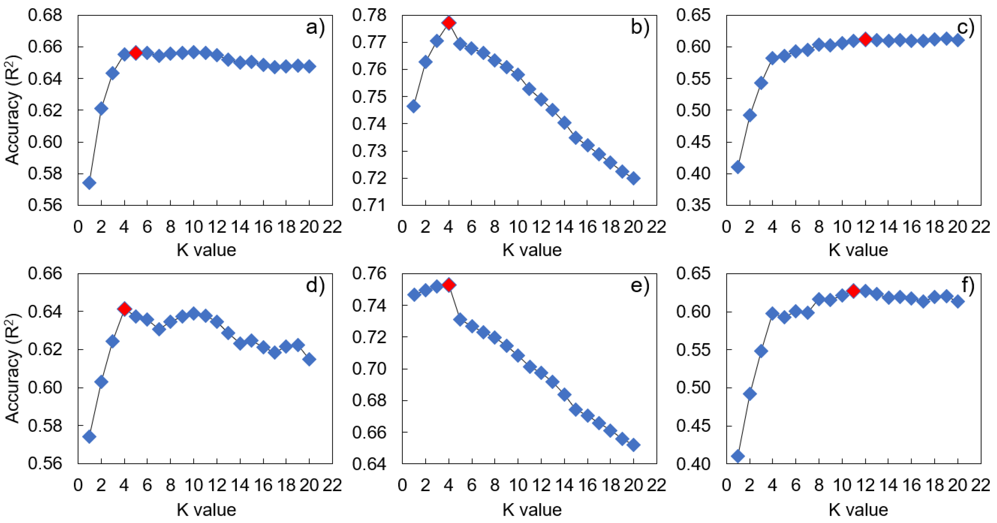
2.3. Hyperparameter Tuning
2.4. Model Validation and Evaluation
3. Results
3.1. Principal Component Analysis
3.2. Input Variable Selection
3.3. Model Performance
3.4. Optimal Model Performance
3.5. Importance of Input Variables in the Optimal Model
4. Discussion and Recommendations
5. Conclusions
Author Contributions
Funding
Institutional Review Board Statement
Informed Consent Statement
Data Availability Statement
Conflicts of Interest
Abbreviations
References
- Zamani Joharestani, M.; Cao, C.; Ni, X.; Bashir, B.; Talebiesfandarani, S. PM2. 5 prediction based on random forest, XGBoost, and deep learning using multisource remote sensing data. Atmosphere 2019, 10, 373. [Google Scholar] [CrossRef]
- Ye, Z.; Yang, J.; Zhong, N.; Tu, X.; Jia, J.; Wang, J. Tackling environmental challenges in pollution controls using artificial intelligence: A review. Sci. Total Environ. 2020, 699, 134279. [Google Scholar] [CrossRef]
- Lu, W.; Lou, J.; Webster, C.; Xue, F.; Bao, Z.; Chi, B. Estimating construction waste generation in the Greater Bay Area, China using machine learning. Waste Manag. 2021, 134, 78–88. [Google Scholar] [CrossRef] [PubMed]
- World Health Organization. Hidden Cities: Unmasking and Overcoming Health Inequities in Urban Settings; World Health Organization: Geneva, Switzerland, 2010. [Google Scholar]
- Leão, S.; Bishop, I.; Evans, D. Spatial-temporal model for demand and allocation of waste landfills in growing urban regions. Comput. Environ. Urban Syst. 2004, 28, 353–385. [Google Scholar] [CrossRef]
- Adeyemi, A.S.; Olorunfemi, J.F.; Adewoye, T.O. Waste Scavenging in third world cities: A case study in Ilorin, Nigeria. Environmentalist 2001, 21, 93–96. [Google Scholar] [CrossRef]
- Esin, T.; Cosgun, N. A study conducted to reduce construction waste generation in Turkey. Build. Environ. 2007, 42, 1667–1674. [Google Scholar] [CrossRef]
- Kontokosta, C.E.; Hong, B.; Johnson, N.E.; Starobin, D. Using machine learning and small area estimation to predict building-level municipal solid waste generation in cities. Comput. Environ. Urban Syst. 2018, 70, 151–162. [Google Scholar] [CrossRef]
- Lu, W.; Yuan, H. Exploring critical success factors for waste management in construction projects of China. Resour. Conserv. Recycl. 2010, 55, 201–208. [Google Scholar] [CrossRef]
- Coelho, A.; de Brito, J. Influence of construction and demolition waste management on the environmental impact of buildings. Waste Manag. 2012, 32, 532–541. [Google Scholar] [CrossRef]
- Lu, W.; Tam, V. Construction waste management policies and their effectiveness in Hong Kong: A longitudinal review. Renew. Sustain. Energy Rev. 2013, 23, 214–223. [Google Scholar] [CrossRef]
- Kulatunga, U.; Amaratunga, D.; Haigh, R.; Rameezdeen, R. Attitudes and perceptions of construction workforce on construction waste in Sri Lanka. Manag. Environ. Qual. Int. J. 2006, 17, 57–72. [Google Scholar] [CrossRef]
- Song, Y.; Wang, Y.; Liu, F.; Zhang, Y. Development of a hybrid model to predict construction and demolition waste: China as a case study. Waste Manag. 2017, 59, 350–361. [Google Scholar] [CrossRef]
- Wu, H.; Zuo, J.; Zillante, G.; Wang, J.; Yuan, H. Status quo and future directions of construction and demolition waste research: A critical review. J. Cleaner Prod. 2019, 240, 118163. [Google Scholar] [CrossRef]
- López-Ruiz, L.A.; Roca-Ramón, X.; Gassó-Domingo, S. The circular economy in the construction and demolition waste sector— A review and an integrative model approach. J. Clean. Prod. 2020, 248, 119238. [Google Scholar] [CrossRef]
- Butera, S.; Christensen, T.H.; Astrup, T.F. Composition and leaching of construction and demolition waste: Inorganic elements and organic compounds. J. Hazard. Mater. 2014, 276, 302–311. [Google Scholar] [CrossRef] [PubMed]
- Lu, W.; Yuan, H.; Li, J.; Hao, J.J.; Mi, X.; Ding, Z. An empirical investigation of construction and demolition waste generation rates in Shenzhen City, South China. Waste Manag. 2011, 31, 680–687. [Google Scholar] [CrossRef] [PubMed]
- Ma, Z.; Shen, J.; Wang, C.; Wu, H. Characterization of Sustainable Mortar Containing High-Quality Recycled Manufactured Sand Crushed from Recycled Coarse Aggregate. Cem. Concr. Compos. 2022, 132, 104629. [Google Scholar] [CrossRef]
- Wu, H.; Xu, J.; Yang, D.; Ma, Z. Utilizing thermal activation treatment to improve the properties of waste cementitious powder and its newmade cementitious materials. J. Clean. Prod. 2021, 322, 129074. [Google Scholar] [CrossRef]
- Abdallah, M.; Talib, M.A.; Feroz, S.; Nasir, Q.; Abdalla, H.; Mahfood, B. Artificial intelligence applications in solid waste management: A systematic research review. Waste Manag. 2020, 109, 231–246. [Google Scholar] [CrossRef]
- Abbasi, M.; Abduli, M.A.; Omidvar, B.; Baghvand, A. Forecasting municipal solid waste generation by hybrid support vector machine and partial least square model. Int. J. Environ. Res. 2013, 7, 27–38. [Google Scholar]
- Abbasi, M.; Abduli, M.A.; Omidvar, B.; Baghvand, A. Results uncertainty of support vector machine and hybrid of wavelet transform-support vector machine models for solid waste generation forecasting. Environ. Prog. Sustain. Energy. 2014, 33, 220–228. [Google Scholar] [CrossRef]
- Soni, U.; Roy, A.; Verma, A.; Jain, V. Forecasting municipal solid waste generation using artificial intelligence models—A case study in India. SN Appl. Sci. 2019, 1, 162. [Google Scholar] [CrossRef]
- Cha, G.W.; Moon, H.J.; Kim, Y.C. A hybrid machine-learning model for predicting the waste generation rate of building demolition projects. J. Cleaner Prod. 2022, 375, 134096. [Google Scholar] [CrossRef]
- Cochran, K.; Townsend, T.; Reinhart, D.; Heck, H. Estimation of regional building-related C&D debris generation and composition: Case study for Florida, US. Waste Manag. 2007, 7, 921–931. [Google Scholar] [CrossRef]
- Kartam, N.; Al-Mutairi, N.; Al-Ghusain, I.; Al-Humoud, J. Environmental management of construction and demolition waste in Kuwait. Waste Manag. 2004, 24, 1049–1059. [Google Scholar] [CrossRef] [PubMed]
- Martínez-Lage, I.; Martínez-Abella, F.; Vázquez-Herrero, C.; Pérez-Ordóñez, J.L. Estimation of the annual production and composition of C&D Debris in Galicia (Spain). Waste Manag. 2010, 30, 636–645. [Google Scholar] [CrossRef]
- Nguyen, X.C.; Nguyen, T.T.H.; La, D.D.; Kumar, G.; Rene, E.R.; Nguyen, D.D.; Chang, S.W.; Chung, W.J.; Nguyen, X.H.; Nguyen, V.K. Development of machine learning-based models to forecast solid waste generation in residential areas: A case study from Vietnam. Resour. Conserv. Recycl. 2021, 167, 105381. [Google Scholar] [CrossRef]
- Abbasi, M.; El Hanandeh, A. Forecasting municipal solid waste generation using artificial intelligence modelling approaches. Waste Manag. 2016, 56, 13–22. [Google Scholar] [CrossRef]
- Çamdevýren, H.; Demýr, N.; Kanik, A.; Keskýn, S. Use of principal component scores in multiple linear regression models for prediction of Chlorophyll-a in reservoirs. Ecol. Model. 2005, 181, 581–589. [Google Scholar] [CrossRef]
- Noori, R.; Abdoli, M.A.; Ameri-Ghasrodashti, A.; Jalili-Ghazizadea, M. Prediction of municipal solid waste generation with combination of support vector machine and principal component analysis: A case study of Mashhad. Env. Progress Sustain. Energy. 2008, 28, 249–258. [Google Scholar] [CrossRef]
- Noori, R.; Karbassi, A.; Salman Sabahi, M.S. Evaluation of PCA and gamma test techniques on ANN operation for weekly solid waste prediction. J. Environ. Manag. 2010, 91, 767–771. [Google Scholar] [CrossRef] [PubMed]
- Khikmah, L.; Wijayanto, H.; Syafitri, U.D. Iop In modeling governance KB with CATPCA to overcome multicollinearity in the logistic regression. In Proceedings of the 3rd International Conference on Mathematics, Science and Education (ICMSE), Semarang, Indonesia, 3–4 September 2016. [Google Scholar]
- Saukani, N.; Ismail, N.A. Identifying the Components of Social Capital by Categorical Principal Component Analysis (CATPCA). Soc. Indic. Res. 2019, 141, 631–655. [Google Scholar] [CrossRef]
- Abdi, H. The method of least squares. In Encyclopedia of Measurement and Statistics; SAGE Publishing: Thousand Oaks, CA, USA, 2007. [Google Scholar]
- Azadi, S.; Karimi-Jashni, A. Verifying the performance of artificial neural network and multiple linear regression in predicting the mean seasonal municipal solid waste generation rate: A case study of Fars province, Iran. Waste Manag. 2016, 48, 14–23. [Google Scholar] [CrossRef]
- Cha, G.W.; Choi, S.H.; Hong, W.H.; Park, C.W. Development of machine learning model for prediction of demolition waste generation rate of buildings in redevelopment areas. Int. J. Environ. Res. Public Health 2023, 20, 107. [Google Scholar] [CrossRef]
- Chhay, L.; Reyad, M.A.H.; Suy, R.; Islam, M.R.; Mian, M.M. Municipal solid waste generation in China: Influencing factor analysis and multi-model forecasting. J. Mater. Cycles Waste Manag. 2018, 20, 1761–1770. [Google Scholar] [CrossRef]
- Fu, H.Z.; Li, Z.S.; Wang, R.H. Estimating municipal solid waste generation by different activities and various resident groups in five provinces of China. Waste Manag. 2015, 41, 3–11. [Google Scholar] [CrossRef]
- Golbaz, S.; Nabizadeh, R.; Sajadi, H.S. Comparative study of predicting hospital solid waste generation using multiple linear regression and artificial intelligence. J. Environ. Health Sci. Eng. 2019, 17, 41–51. [Google Scholar] [CrossRef]
- Kumar, A.; Samadder, S.R. An empirical model for prediction of household solid waste generation rate–A case study of Dhanbad, India. Waste Manag. 2017, 68, 3–15. [Google Scholar] [CrossRef] [PubMed]
- Guo, G.; Wang, H.; Bell, D.A.; Bi, Y.; Greer, K. KNN Model-Based Approach in Classification. In Lecture Notes in Computer Science; Springer: Berlin/Heidelberg, Germany, 2003; Volume 2888, pp. 986–996. [Google Scholar] [CrossRef]
- Safavian, S.R.; Landgrebe, D. A survey of decision tree classifier methodology. IEEE Trans. Syst. Man Cybern. 1991, 21, 660–674. [Google Scholar] [CrossRef]
- Hastie, T.J.; Tibshirani, R.J.; Friedman, J.H. The Elements of Statistical Learning: Data Mining, Inference, and Prediction; Springer: New York, NY, USA, 2009. [Google Scholar]
- Cha, G.W.; Kim, Y.C.; Moon, H.J.; Hong, W.H. New approach for forecasting demolition waste generation using chi-squared automatic interaction detection (CHAID) method. J. Cleaner Prod. 2017, 168, 375–385. [Google Scholar] [CrossRef]
- Kuritcyn, P.; Anding, K.; Linß, E.; Latyev, S.M. Increasing the safety in recycling of construction and demolition waste by using supervised machine learning. J. Phys. Conf. Ser. 2015, 588, 012035. [Google Scholar] [CrossRef]
- Huang, X.; Xu, X. Legal regulation perspective of eco-efficiency construction waste reduction and utilization. Urban Dev. Stud. 2011, 9, 90–94. [Google Scholar]
- Kannangara, M.; Dua, R.; Ahmadi, L.; Bensebaa, F. Modeling and prediction of regional municipal solid waste generation and diversion in Canada using machine learning approaches. Waste Manag. 2018, 74, 3–15. [Google Scholar] [CrossRef]
- Shawi, R.E.; Maher, M.; Sakr, S. Automated machine learning: State-of-the-art and open challenges. arXiv 2019, arXiv:1906.02287. [Google Scholar] [CrossRef]
- Cha, G.W.; Moon, H.J.; Kim, Y.M.; Hong, W.H.; Hwang, J.H.; Park, W.J.; Kim, Y.C. Development of a prediction model for demolition waste generation using a random forest algorithm based on small datasets. Int. J. Environ. Res. Public Health 2020, 17, 6997. [Google Scholar] [CrossRef]
- Cha, G.W.; Moon, H.J.; Kim, Y.C. Comparison of random forest and gradient boosting machine models for predicting demolition waste based on small datasets and categorical variables. Int. J. Environ. Res. Public Health 2021, 18, 8530. [Google Scholar] [CrossRef]
- Cheng, H.; Garrick, D.J.; Fernando, R.L. Efficient strategies for leave-one-out cross validation for genomic best linear unbiased prediction. J. Anim. Sci. Biotechnol. 2017, 8, 38. [Google Scholar] [CrossRef]
- Shao, Z.; Er, M.J. Efficient leave-one-out cross-validation-based regularized extreme learning machine. Neurocomputing. 2016, 194, 260–270. [Google Scholar] [CrossRef]
- Cheng, J.; Dekkers, J.C.; Fernando, R.L. Cross-validation of best linear unbiased predictions of breeding values using an efficient leave-one-out strategy. J. Anim. Breed. Genet. 2021, 138, 519–527. [Google Scholar] [CrossRef] [PubMed]
- Wong, T.T. Performance evaluation of classification algorithms by k-fold and leave-one-out cross validation. Pattern Recognit. 2015, 48, 2839–2846. [Google Scholar] [CrossRef]
- Sun, N.C.S.; Chungpaibulpatana, S. Development of an appropriate model for forecasting municipal solid waste generation in Bangkok. Energy Procedia 2017, 138, 907–912. [Google Scholar] [CrossRef]
- Shi, Y.; Wang, Y.; Yue, Y.; Zhao, J.; Maraseni, T.; Qian, G. Unbalanced Status and Multidimensional Influences of Municipal Solid Waste Management in Africa. Chemosphere 2021, 281, 130884. [Google Scholar] [CrossRef] [PubMed]


| Category | Number of Buildings | Total Demolition Waste Generation (kg) | DWGR (kg·m−2) | GFA (m2) | |||
|---|---|---|---|---|---|---|---|
| Min | Mean | Max | |||||
| Location | Project A | 81 | 6,072,522 | 534.8 | 741.6 | 1137.3 | 8301.0 |
| Project B | 79 | 18,194,868 | 795.2 | 1238.9 | 1729.1 | 13,627.3 | |
| Usage | Residential | 135 | 17,875,051 | 534.8 | 938.0 | 1629.4 | 16,994.4 |
| Mixed-use (residential & commercial) | 25 | 6,392,340 | 750.9 | 1253.0 | 1729.1 | 4933.8 | |
| Structure | Reinforced Concrete | 35 | 12,573,029 | 795.2 | 1430.4 | 1637.0 | 8652.1 |
| Concrete block | 81 | 6,360,974 | 534.8 | 854.6 | 1180.5 | 7539.8 | |
| Concrete brick | 15 | 3,050,583 | 717.0 | 1452.1 | 1729.1 | 2500.4 | |
| Wood | 29 | 2,282,804 | 590.5 | 755.4 | 883.0 | 3236.0 | |
| Wall type | Brick | 32 | 4,727,204 | 590.5 | 995.9 | 1729.1 | 4556.0 |
| Block | 121 | 18,975,282 | 534.8 | 1000.8 | 1637.0 | 16,579.0 | |
| Soil | 7 | 564,904 | 668.0 | 711.8 | 759.8 | 4556.0 | |
| Roof type | Slab | 37 | 9,062,146 | 717.0 | 1228.3 | 1729.1 | 7003.5 |
| Slab and roofing tile | 33 | 6,939,655 | 931.0 | 1213.2 | 1637.0 | 5080.8 | |
| Slab & slate | 3 | 963,912 | 813.5 | 1310.3 | 1614.8 | 719.6 | |
| Slate | 13 | 841,899 | 534.8 | 599.7 | 681.8 | 1384.9 | |
| Roofing tile | 74 | 6,459,779 | 580.0 | 820.8 | 1576.5 | 7739.5 | |
| Machine-Learning Algorithms | Hyperparameters | ||||
|---|---|---|---|---|---|
| Title | Tested Values | Selected | |||
| KNN | Euclidean | distance | K neighbors | Range (1, 20) | 5 |
| Manhattan | 4 | ||||
| Chebyshev | 12 | ||||
| Euclidean | uniform | 4 | |||
| Manhattan | 4 | ||||
| Chebyshev | 11 | ||||
| LR | Ridge | alpha | Range (0.0001, 1000) | 0.5 | |
| Lasso | 0.8 | ||||
| Elastic net | 0.6 | ||||
| DT | Min samples leaf | Range (1, 10) | 2 | ||
| Split criteria | Range (1, 10) | 1 | |||
| Max depth | Range (1, 15) | 4 | |||
| Variables | Loading of Variables | ||||||||||||
|---|---|---|---|---|---|---|---|---|---|---|---|---|---|
| PC 1 | PC 2 | PC 3 | PC 4 | PC 5 | PC 6 | PC 7 | PC 8 | PC 9 | PC 10 | PC 11 | PC 12 | PC 13 | |
| Location_project A | 0.29 | −0.28 | 0.00 | −0.29 | −0.04 | 0.05 | 0.02 | 0.17 | 0.36 | −0.26 | 0.13 | −0.08 | 0.02 |
| Location_project B | −0.29 | 0.28 | 0.00 | 0.29 | 0.04 | −0.05 | −0.02 | −0.17 | −0.36 | 0.26 | −0.13 | 0.08 | −0.02 |
| Floor area | 0.31 | −0.10 | 0.32 | 0.22 | −0.01 | −0.11 | −0.03 | −0.11 | −0.22 | −0.20 | −0.19 | −0.45 | −0.63 |
| Usage_residential | −0.30 | −0.15 | 0.17 | 0.01 | −0.27 | −0.24 | 0.39 | 0.21 | −0.02 | −0.11 | −0.11 | 0.04 | 0.00 |
| Usage_residential & commercial | 0.30 | 0.15 | −0.17 | −0.01 | 0.27 | 0.24 | −0.39 | −0.21 | 0.02 | 0.11 | 0.11 | −0.04 | 0.00 |
| Structure_concrete block | −0.24 | −0.24 | −0.43 | −0.02 | 0.10 | 0.06 | −0.12 | 0.18 | 0.11 | 0.10 | −0.22 | 0.11 | −0.43 |
| Structure_concrete brick | 0.21 | 0.27 | −0.33 | −0.07 | −0.13 | −0.07 | 0.06 | 0.16 | −0.51 | −0.45 | 0.05 | −0.19 | 0.29 |
| Structure_reinforced concrete | 0.28 | −0.19 | 0.36 | 0.22 | 0.06 | −0.10 | 0.03 | −0.07 | 0.12 | 0.30 | −0.27 | −0.12 | 0.49 |
| Structure_wood | −0.14 | 0.31 | 0.42 | −0.15 | −0.10 | 0.09 | 0.08 | −0.28 | 0.11 | −0.11 | 0.53 | 0.14 | −0.19 |
| Wall type_block | −0.13 | −0.44 | −0.01 | 0.17 | 0.16 | −0.17 | −0.15 | −0.09 | −0.21 | −0.10 | 0.36 | 0.02 | 0.09 |
| Wall type_brick | 0.17 | 0.39 | −0.16 | −0.15 | −0.01 | −0.01 | 0.38 | −0.17 | 0.26 | 0.07 | −0.32 | −0.02 | −0.10 |
| Wall type_soil | −0.07 | 0.18 | 0.33 | −0.06 | −0.32 | 0.38 | −0.44 | 0.52 | −0.08 | 0.07 | −0.15 | 0.00 | 0.00 |
| Roof type_roofing tile | −0.27 | 0.16 | 0.18 | −0.18 | 0.41 | −0.26 | −0.24 | 0.00 | 0.12 | −0.32 | −0.24 | −0.06 | 0.09 |
| Roof type_slab | 0.29 | 0.14 | −0.13 | 0.16 | −0.17 | −0.36 | 0.03 | 0.34 | 0.05 | 0.40 | 0.36 | 0.01 | −0.15 |
| Roof type_slab/roofing tile | 0.06 | −0.33 | 0.00 | −0.41 | −0.29 | 0.29 | 0.10 | −0.35 | −0.36 | 0.19 | −0.11 | 0.07 | −0.01 |
| Roof type_slab/slate | 0.09 | −0.03 | 0.14 | 0.15 | 0.54 | 0.48 | 0.48 | 0.34 | −0.18 | −0.02 | 0.09 | 0.11 | −0.05 |
| Roof type_slate | −0.10 | −0.02 | −0.18 | 0.61 | −0.32 | 0.37 | 0.02 | −0.18 | 0.31 | −0.31 | 0.01 | −0.07 | 0.09 |
| Number of floors | 0.36 | −0.02 | 0.10 | 0.15 | −0.06 | −0.14 | −0.10 | −0.03 | −0.08 | −0.27 | −0.20 | 0.82 | −0.10 |
| Model | Input Variables | |
|---|---|---|
| Non-hybrid | LR | location, usage, structure, wall type, roof type, number of floors, floor area |
| LR (ridge) | ||
| LR (lasso) | ||
| LR (elastic net) | ||
| KNN (Euclidean distance) | ||
| KNN (Manhattan distance) | ||
| KNN (Chebyshev distance) | ||
| KNN (Euclidean uniform) | ||
| KNN (Manhattan uniform) | ||
| KNN (Chebyshev uniform) | ||
| DT | ||
| Hybrid | LR | PC 1, 2, 3, 4, 6, 8, 9, 10, 11, 13 |
| LR (ridge) | PC 1, 2, 3, 4, 6, 8, 9, 10, 11, 13 | |
| LR (lasso) | PC 1, 2, 3, 4, 6, 8, 9, 10, 11, 13, location, number of floors | |
| LR (elastic net) | PC 1, 2, 3, 4, 6, 8, 9, 10, 11, 13, location, number of floors | |
| KNN (Euclidean distance) | PC 1, 2, location, structure, wall type, floor area | |
| KNN (Manhattan distance) | PC 1, 2, 4, location, wall type, structure, floor area | |
| KNN (Chebyshev distance) | PC 1, 2, 4, wall type, structure | |
| KNN (Euclidean uniform) | PC 1, 2, 4, structure, wall type, floor area, number of floors | |
| KNN (Manhattan uniform) | PC 1, 2, 4, location, wall type, structure, floor area, number of floors | |
| KNN (Chebyshev uniform) | PC 1,2,4, location, structure, wall type, floor area | |
| DT | PC 1, 2, 5, 10, 13 | |
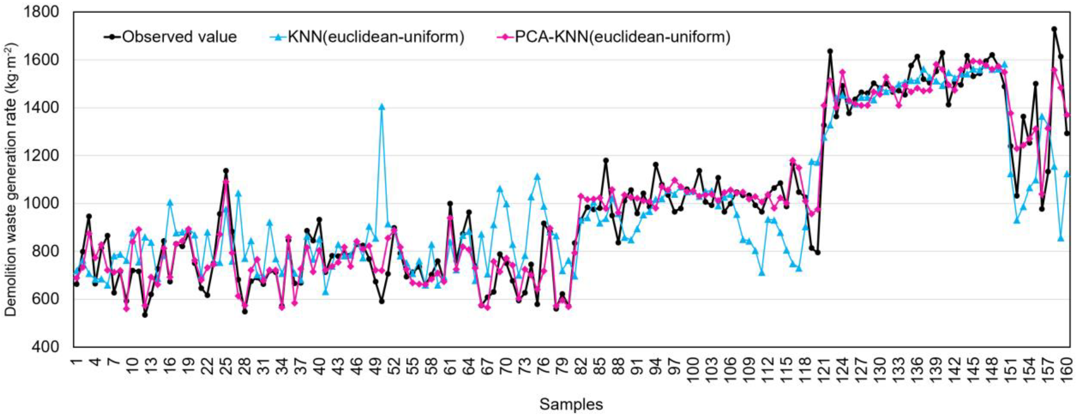
| Model Type | Input Variables | Pearson’s Correlation |
|---|---|---|
| KNN (Euclidean uniform) | number of floors | 0.782 |
| floor area | 0.747 | |
| usage | 0.359 | |
| structure | 0.172 | |
| roof type | 0.107 | |
| wall type | −0.130 | |
| location | −0.782 | |
| PCA−KNN (Euclidean uniform) | PC1 | 0.783 |
| number of floors | 0.782 | |
| floor area | 0.747 | |
| structure | 0.172 | |
| PC4 | −0.117 | |
| wall type | −0.130 | |
| PC2 | −0.377 |
Disclaimer/Publisher’s Note: The statements, opinions and data contained in all publications are solely those of the individual author(s) and contributor(s) and not of MDPI and/or the editor(s). MDPI and/or the editor(s) disclaim responsibility for any injury to people or property resulting from any ideas, methods, instructions or products referred to in the content. |
© 2023 by the authors. Licensee MDPI, Basel, Switzerland. This article is an open access article distributed under the terms and conditions of the Creative Commons Attribution (CC BY) license (https://creativecommons.org/licenses/by/4.0/).
Share and Cite
Cha, G.-W.; Choi, S.-H.; Hong, W.-H.; Park, C.-W. Developing a Prediction Model of Demolition-Waste Generation-Rate via Principal Component Analysis. Int. J. Environ. Res. Public Health 2023, 20, 3159. https://doi.org/10.3390/ijerph20043159
Cha G-W, Choi S-H, Hong W-H, Park C-W. Developing a Prediction Model of Demolition-Waste Generation-Rate via Principal Component Analysis. International Journal of Environmental Research and Public Health. 2023; 20(4):3159. https://doi.org/10.3390/ijerph20043159
Chicago/Turabian StyleCha, Gi-Wook, Se-Hyu Choi, Won-Hwa Hong, and Choon-Wook Park. 2023. "Developing a Prediction Model of Demolition-Waste Generation-Rate via Principal Component Analysis" International Journal of Environmental Research and Public Health 20, no. 4: 3159. https://doi.org/10.3390/ijerph20043159
APA StyleCha, G.-W., Choi, S.-H., Hong, W.-H., & Park, C.-W. (2023). Developing a Prediction Model of Demolition-Waste Generation-Rate via Principal Component Analysis. International Journal of Environmental Research and Public Health, 20(4), 3159. https://doi.org/10.3390/ijerph20043159