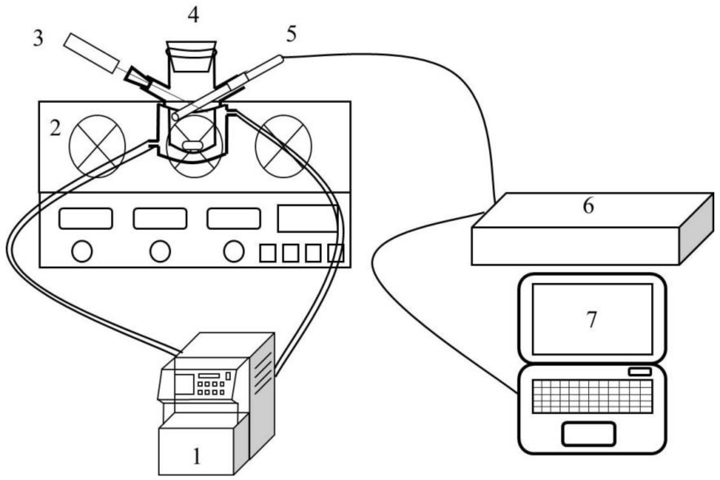
Figure 1.
Metastable zone determination experimental flow chart (1: cooling circulating water machine, 2: digital magnetic stirrer, 3: digital thermometer, 4: crystallizer, 5: FBRM probe, 6: FBRM workstation, 7: computer).
Figure 1.
Metastable zone determination experimental flow chart (1: cooling circulating water machine, 2: digital magnetic stirrer, 3: digital thermometer, 4: crystallizer, 5: FBRM probe, 6: FBRM workstation, 7: computer).
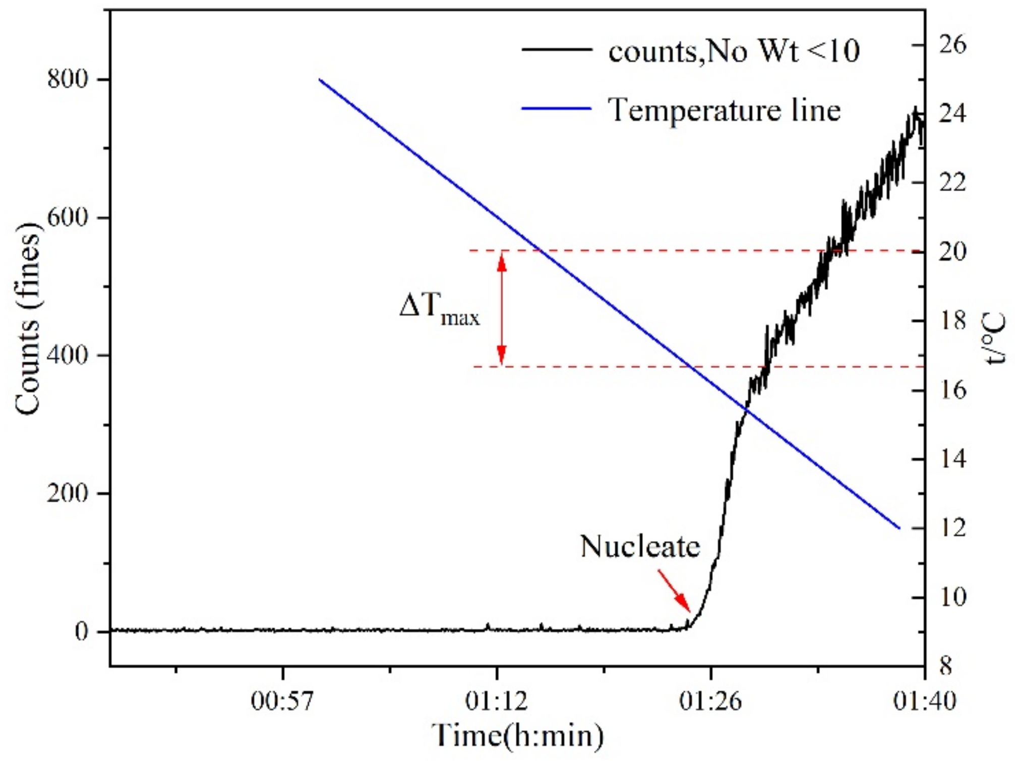
Figure 2.
Schematic diagram of measuring the metastable zone by the Focused Beam Reflectance Meter (FBRM) (taking the saturation temperature of 293.15 K, stirring rate of 300 rpm, ethanol mass fraction of 0.6, and cooling rate of 20 K/h as an example).
Figure 2.
Schematic diagram of measuring the metastable zone by the Focused Beam Reflectance Meter (FBRM) (taking the saturation temperature of 293.15 K, stirring rate of 300 rpm, ethanol mass fraction of 0.6, and cooling rate of 20 K/h as an example).
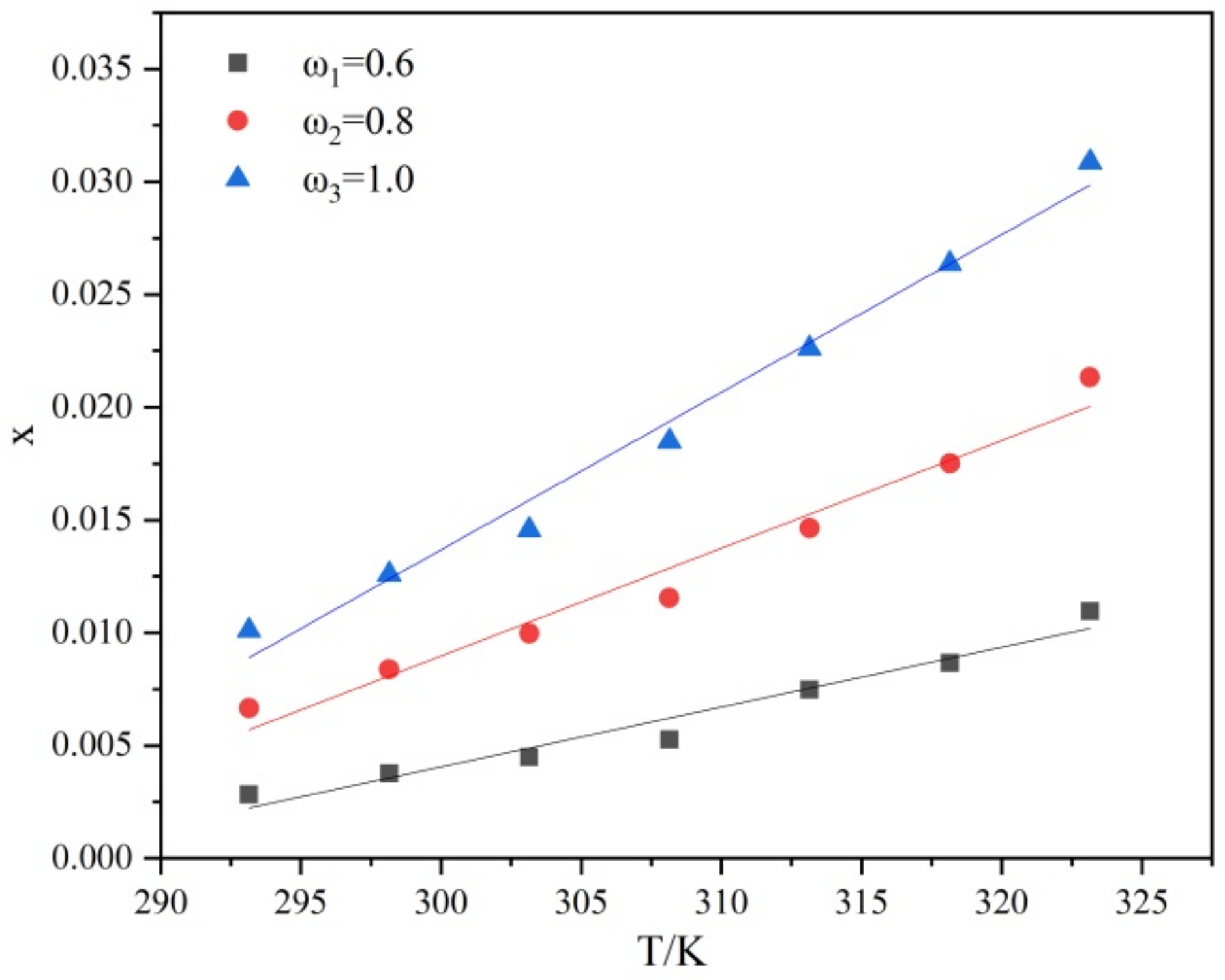
Figure 3.
Relationship between solubility and temperature of PMBA under different ethanol mass fractions.
Figure 3.
Relationship between solubility and temperature of PMBA under different ethanol mass fractions.
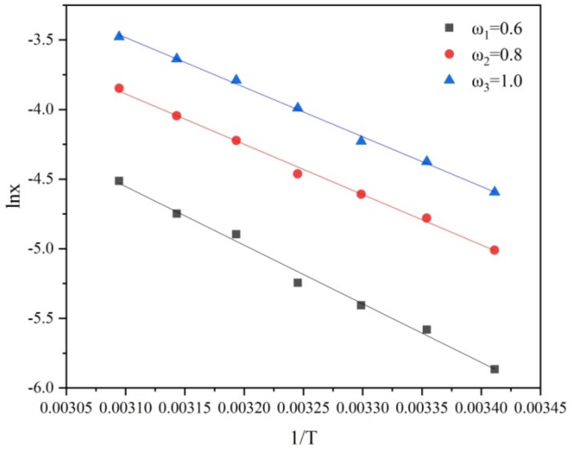
Figure 4.
Solubility of PMBA at different ethanol mass fractions fitted by the Van’t Hoff equation.
Figure 4.
Solubility of PMBA at different ethanol mass fractions fitted by the Van’t Hoff equation.
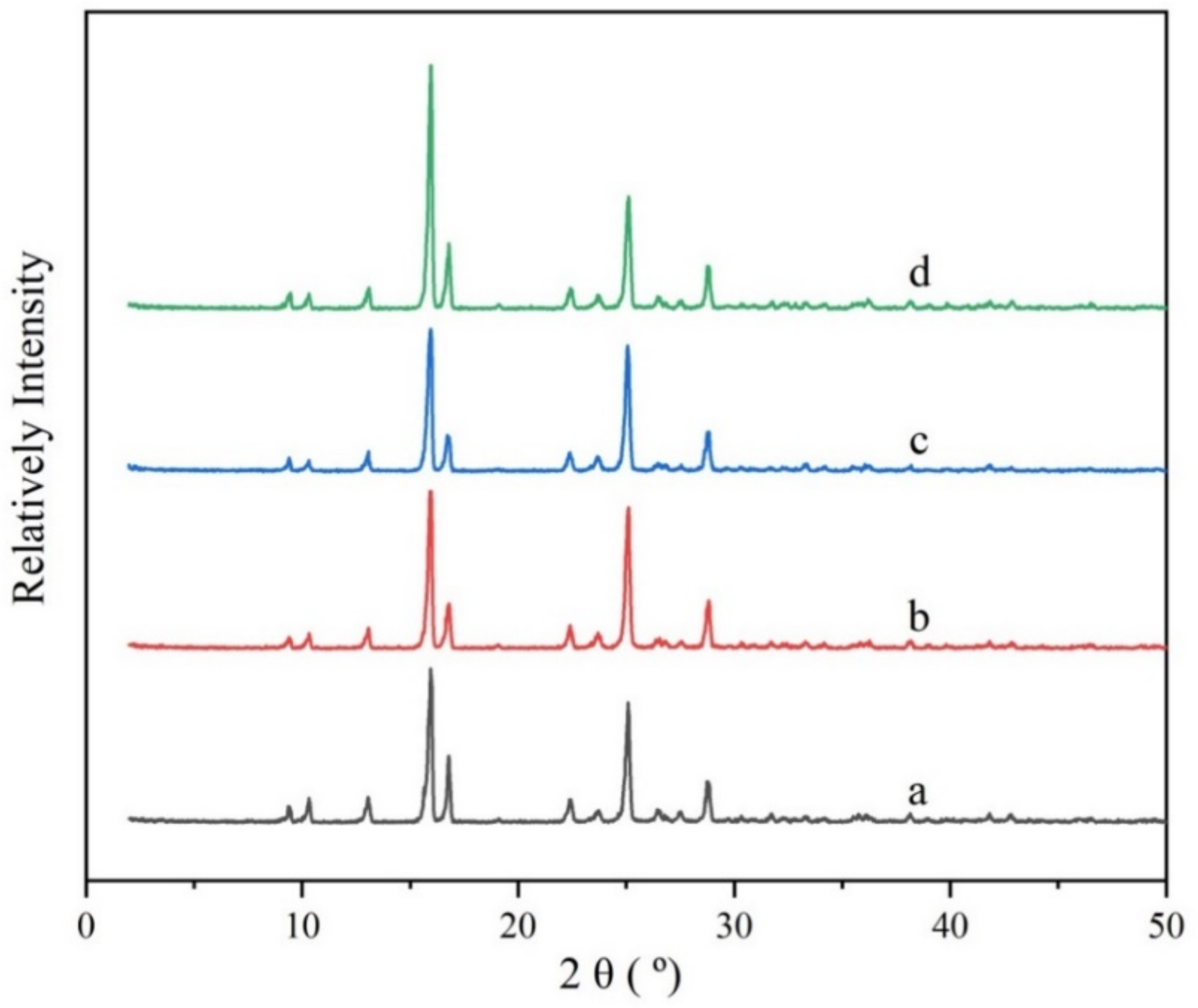
Figure 5.
X-ray powder diffraction patterns of the PMBA solid samples. (a) is the raw material; (b–d) stands for the PXRD patterns of the samples obtained from solvent with ethanol mass fractions of 0.6, 0.8, and 1.0, respectively.
Figure 5.
X-ray powder diffraction patterns of the PMBA solid samples. (a) is the raw material; (b–d) stands for the PXRD patterns of the samples obtained from solvent with ethanol mass fractions of 0.6, 0.8, and 1.0, respectively.
Figure 6.
Relationship between MSZW and cooling rate at different saturation temperatures fitted by Nývlt’s model: (a) ethanol mass fraction of 0.6, (b) ethanol mass fraction of 0.8, and (c) ethanol mass fraction of 1.0.
Figure 6.
Relationship between MSZW and cooling rate at different saturation temperatures fitted by Nývlt’s model: (a) ethanol mass fraction of 0.6, (b) ethanol mass fraction of 0.8, and (c) ethanol mass fraction of 1.0.
Figure 7.
Relationship between MSZW and cooling rate at different saturation temperatures fitted by the Sangwal model: (a) ethanol mass fraction of 0.6, (b) ethanol mass fraction of 0.8, and (c) ethanol mass fraction of 1.0.
Figure 7.
Relationship between MSZW and cooling rate at different saturation temperatures fitted by the Sangwal model: (a) ethanol mass fraction of 0.6, (b) ethanol mass fraction of 0.8, and (c) ethanol mass fraction of 1.0.
Figure 8.
Crystal morphology of PMBA at ethanol mass fraction of (a) 0.6, (b) 0.8, and (c) 1.0 (saturation temperature 293.15 K, cooling rate 20 K/h, the scale in all figures is 20 µm).
Figure 8.
Crystal morphology of PMBA at ethanol mass fraction of (a) 0.6, (b) 0.8, and (c) 1.0 (saturation temperature 293.15 K, cooling rate 20 K/h, the scale in all figures is 20 µm).
Figure 9.
Relationship between MSZW and cooling rate at different fitted by the modified Sangwal model: (a) ethanol mass fraction of 0.6, (b) ethanol mass fraction of 0.8, and (c) ethanol mass fraction of 1.0.
Figure 9.
Relationship between MSZW and cooling rate at different fitted by the modified Sangwal model: (a) ethanol mass fraction of 0.6, (b) ethanol mass fraction of 0.8, and (c) ethanol mass fraction of 1.0.
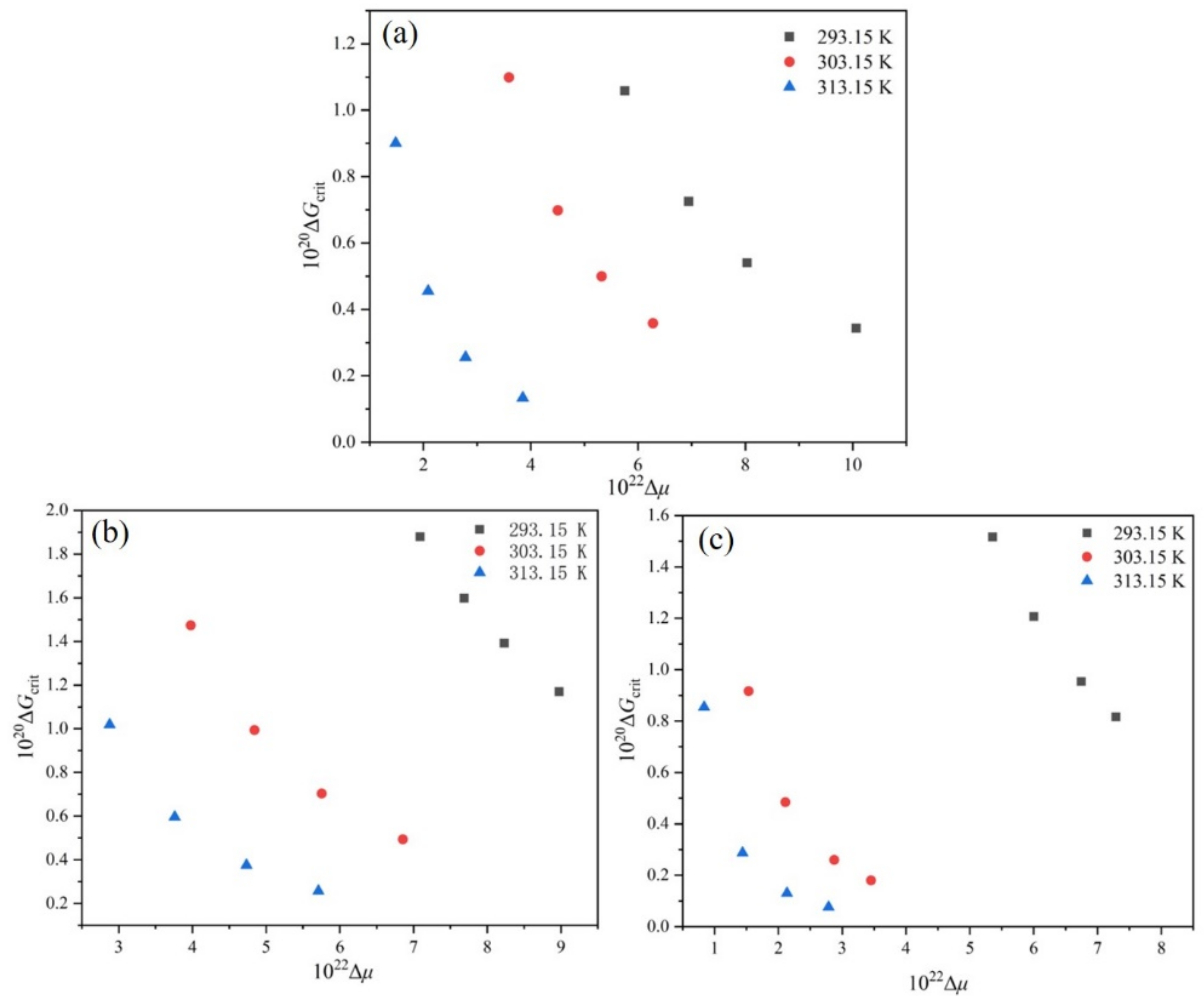
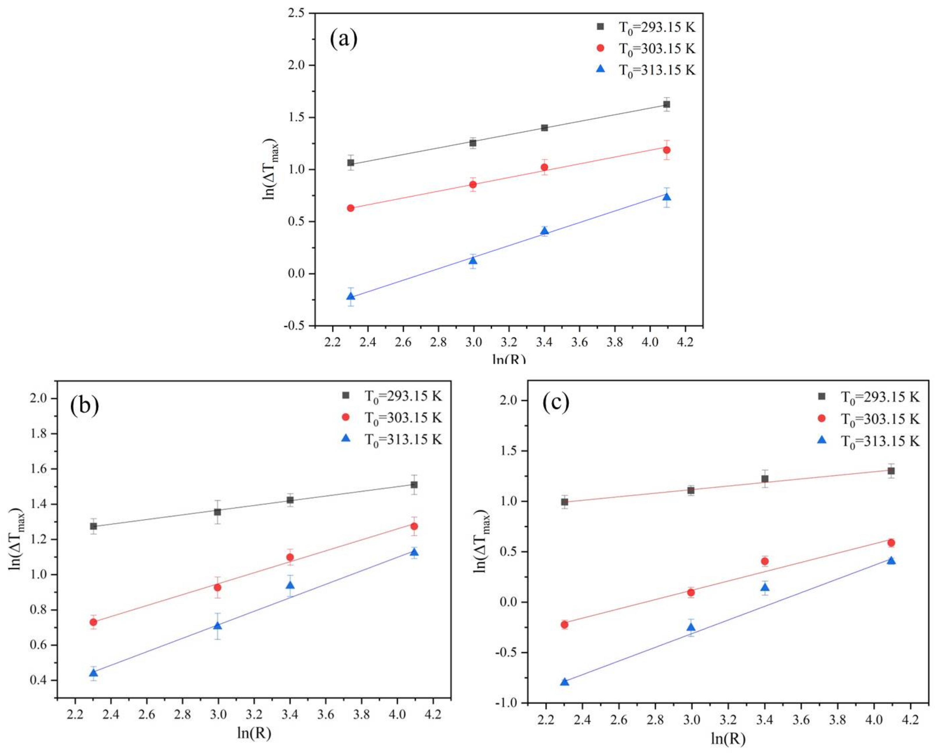
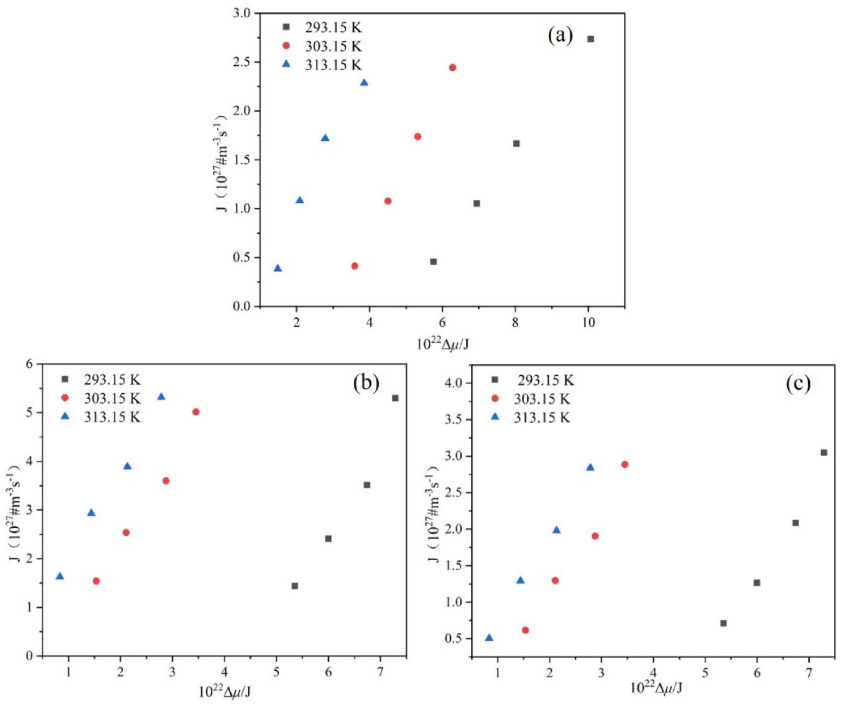
Figure 10.
Relation between and at different : (a) ethanol mass fraction of 0.6, (b) ethanol mass fraction of 0.8, (c) ethanol mass fraction of 1.0.
Figure 10.
Relation between and at different : (a) ethanol mass fraction of 0.6, (b) ethanol mass fraction of 0.8, (c) ethanol mass fraction of 1.0.
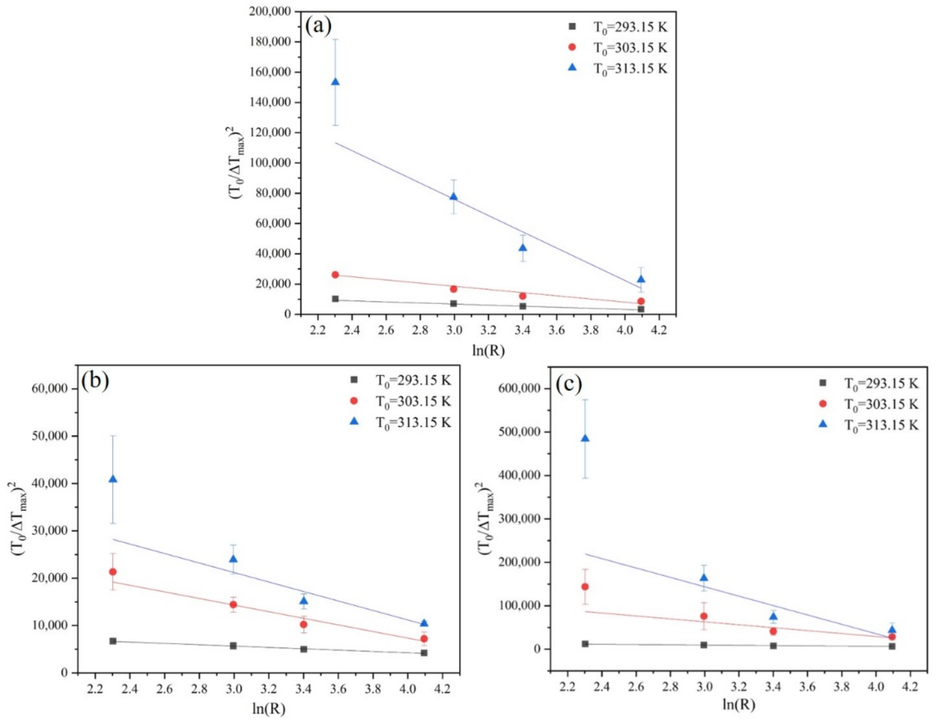
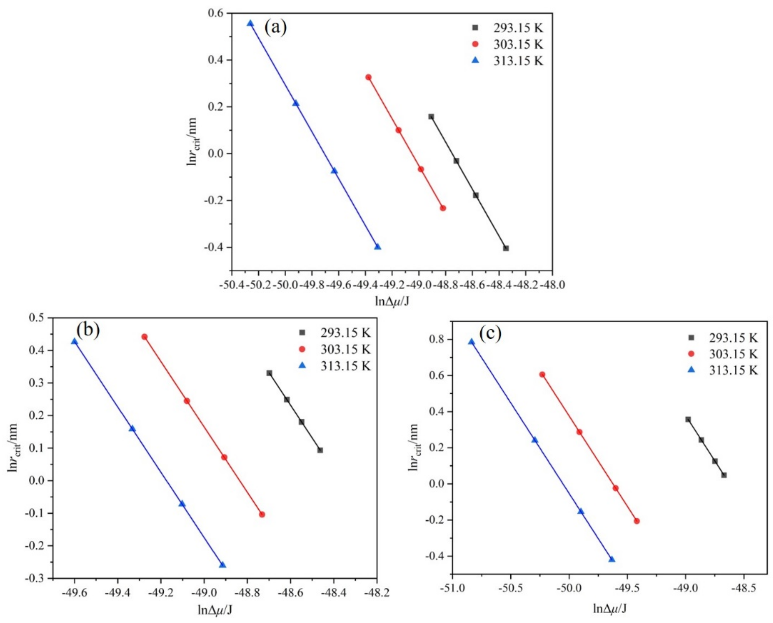
Figure 11.
Relationship between and at different : (a) ethanol mass fraction of 0.6, (b) ethanol mass fraction of 0.8, (c) ethanol mass fraction of 1.0.
Figure 11.
Relationship between and at different : (a) ethanol mass fraction of 0.6, (b) ethanol mass fraction of 0.8, (c) ethanol mass fraction of 1.0.
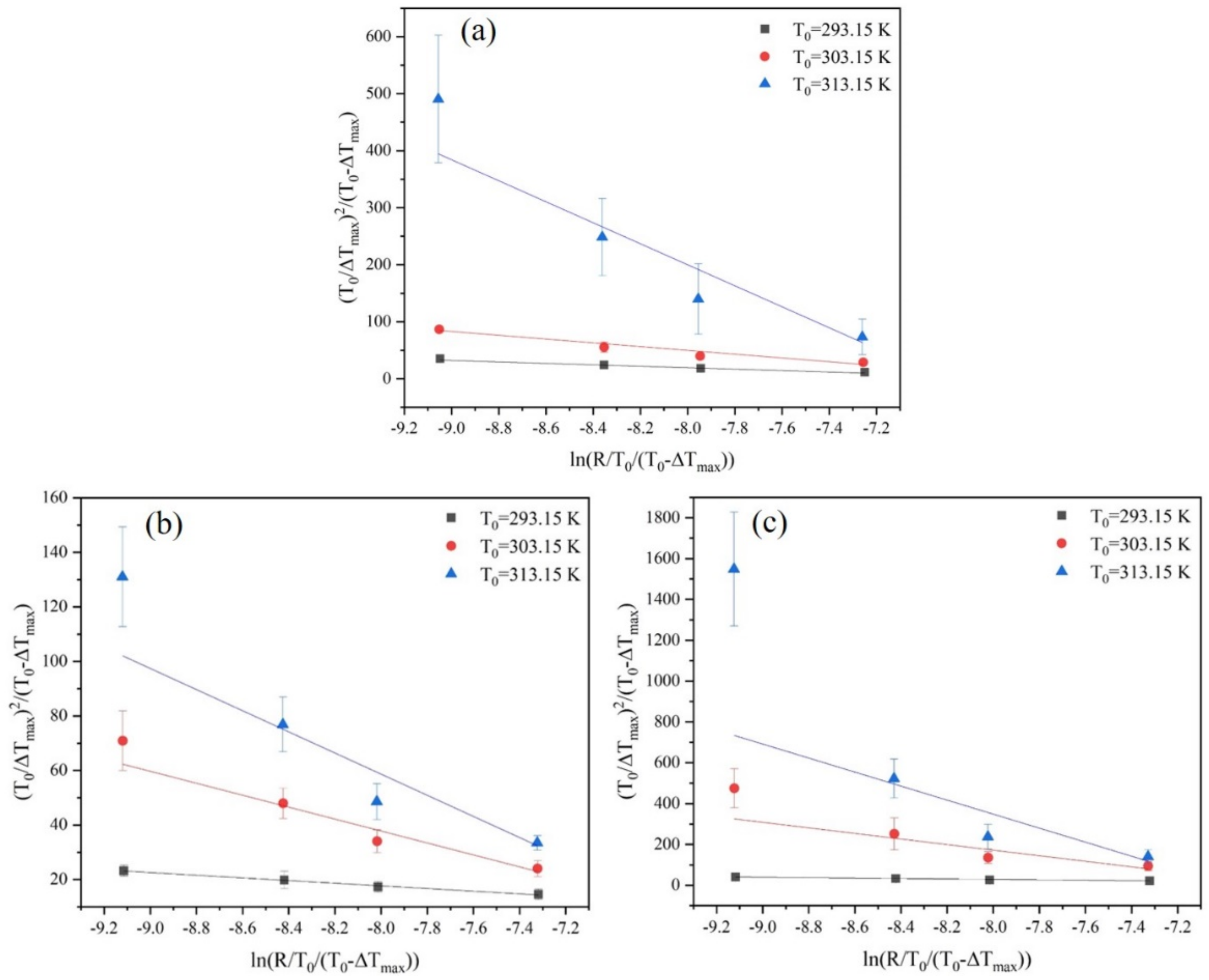
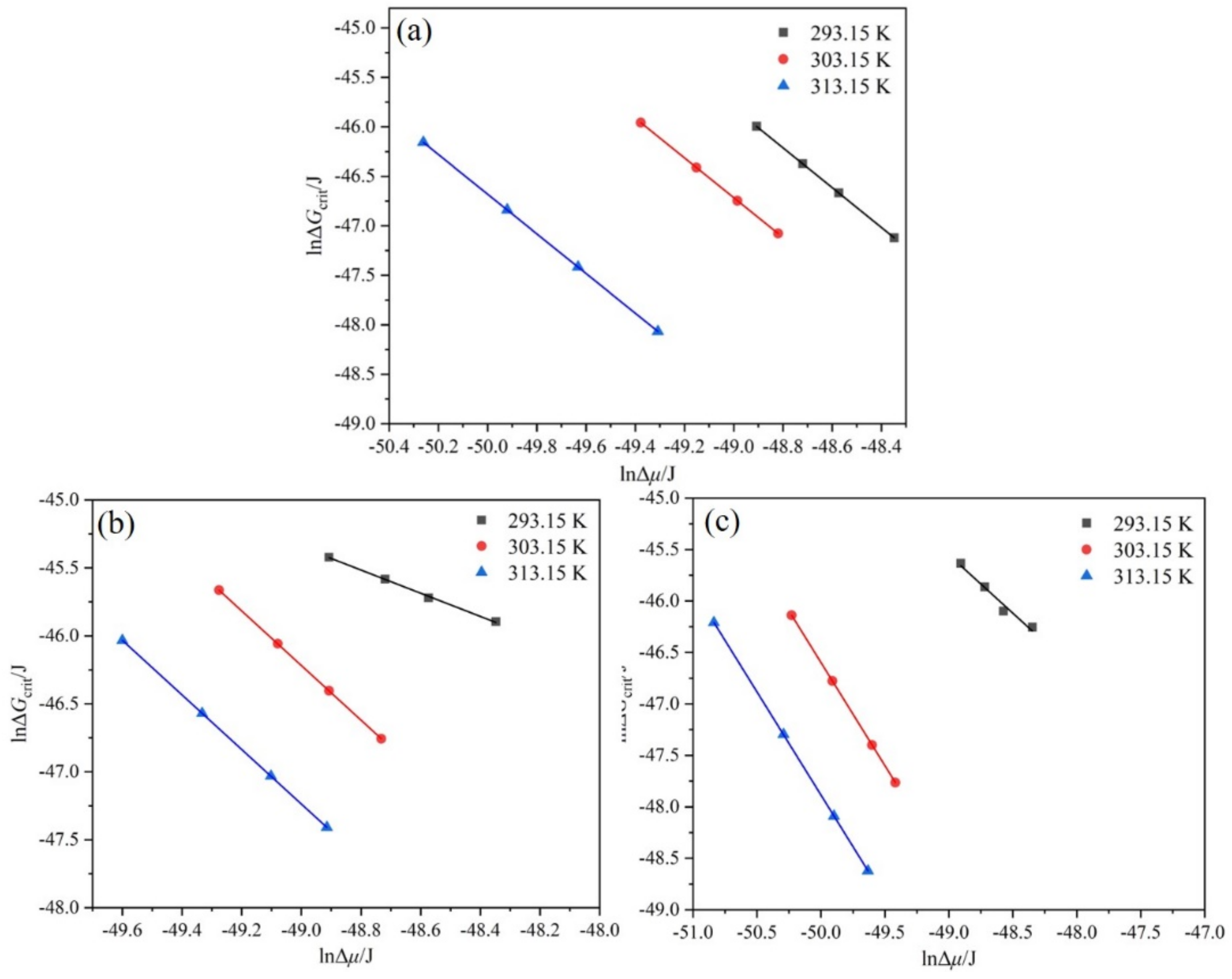
Figure 12.
Relationship between and at different : (a) ethanol mass fraction of 0.6, (b) ethanol mass fraction of 0.8, (c) ethanol mass fraction of 1.0.
Figure 12.
Relationship between and at different : (a) ethanol mass fraction of 0.6, (b) ethanol mass fraction of 0.8, (c) ethanol mass fraction of 1.0.
Figure 13.
Relationship between and at different : (a) ethanol mass fraction of 0.6, (b) ethanol mass fraction of 0.8, (c) ethanol mass fraction of 1.0.
Figure 13.
Relationship between and at different : (a) ethanol mass fraction of 0.6, (b) ethanol mass fraction of 0.8, (c) ethanol mass fraction of 1.0.
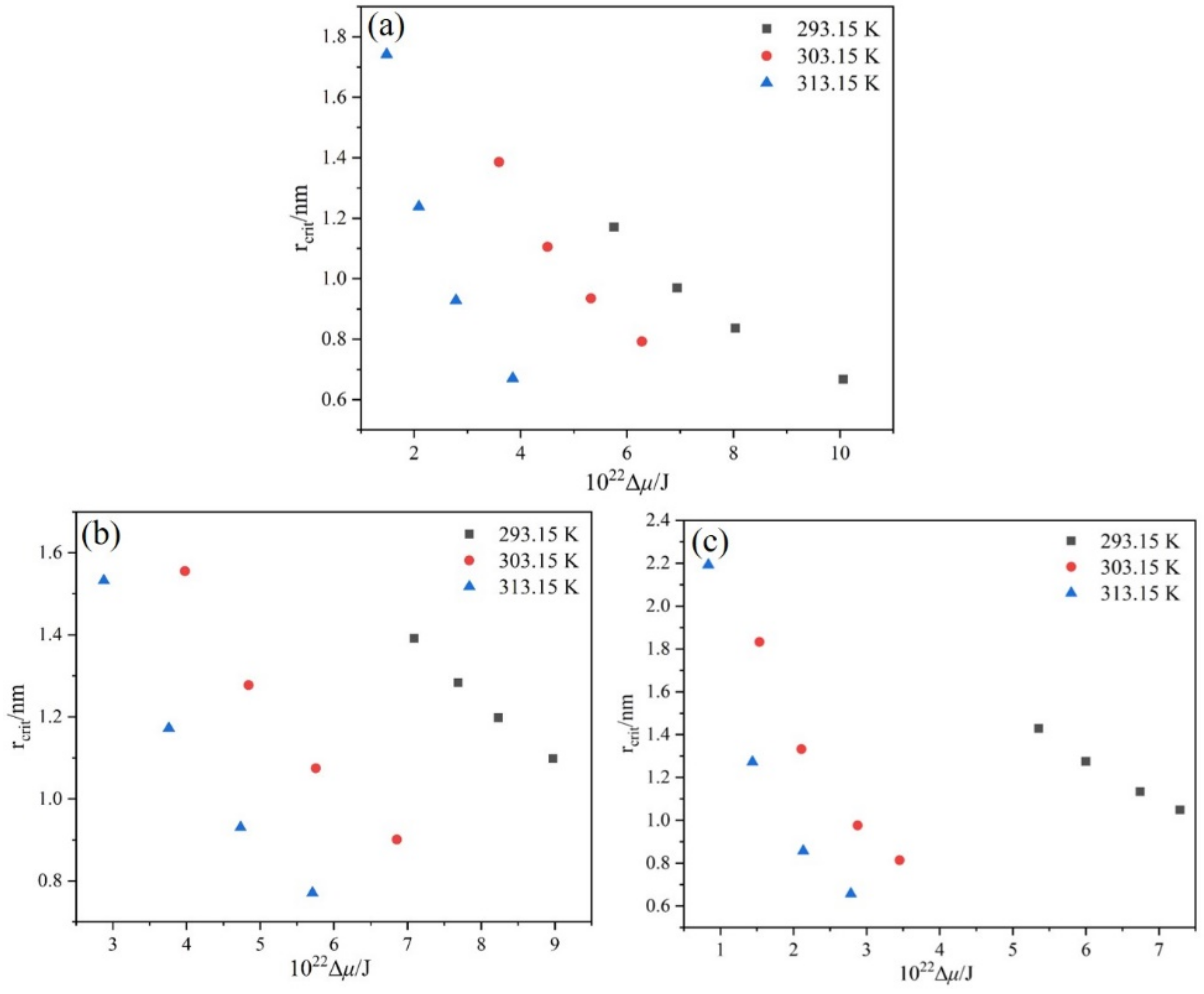
Figure 14.
Relationship between and at different : (a) ethanol mass fraction of 0.6, (b) ethanol mass fraction of 0.8, (c) ethanol mass fraction of 1.0.
Figure 14.
Relationship between and at different : (a) ethanol mass fraction of 0.6, (b) ethanol mass fraction of 0.8, (c) ethanol mass fraction of 1.0.
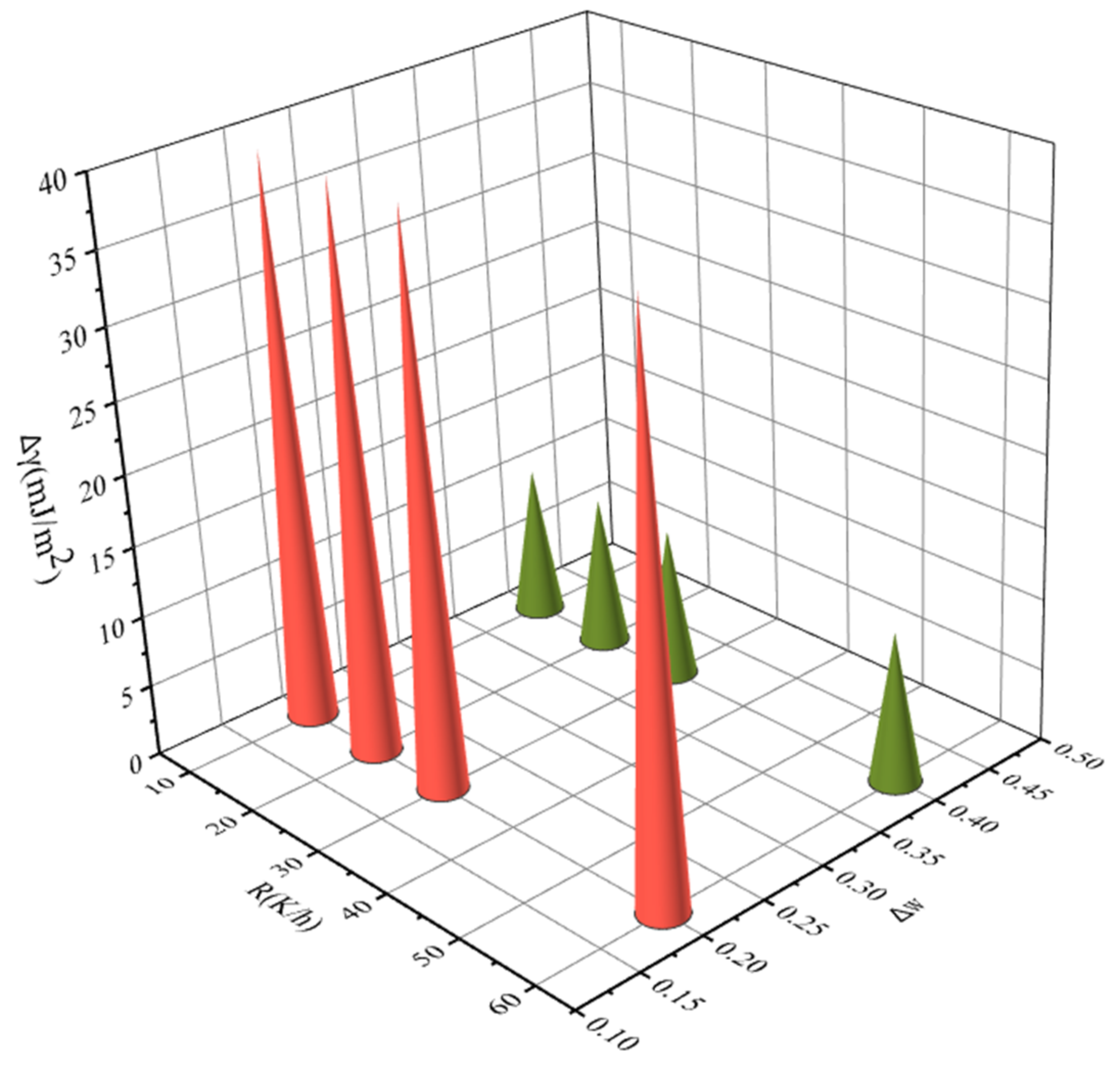
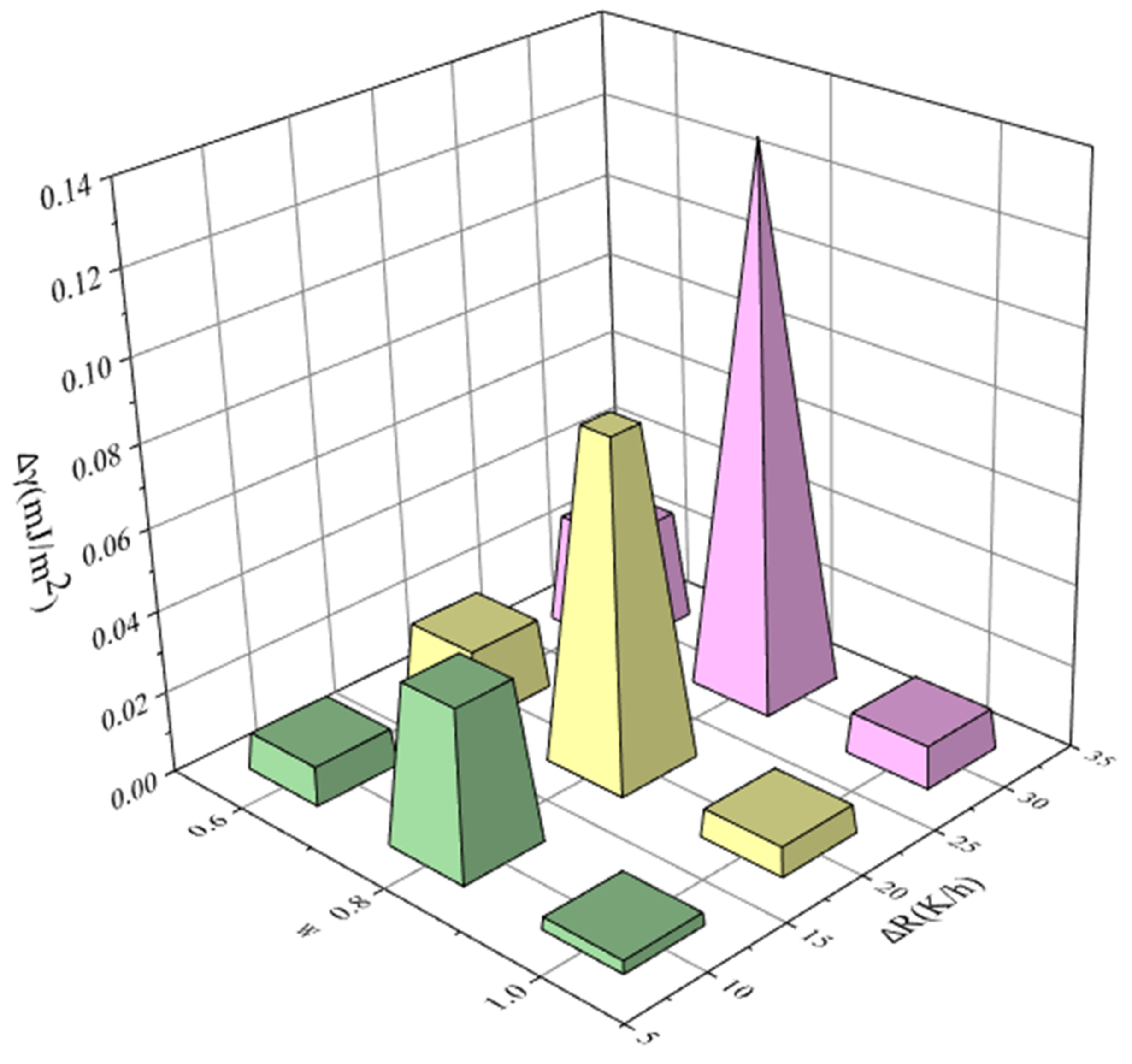
Figure 15.
The relationship between interfacial energy and the change in ethanol mass fraction (saturated temperature 293.15 K, cooling rate 10, 20, 30, and 60 K/h, respectively).
Figure 15.
The relationship between interfacial energy and the change in ethanol mass fraction (saturated temperature 293.15 K, cooling rate 10, 20, 30, and 60 K/h, respectively).
Figure 16.
The relationship between interfacial energy and the change in saturated temperature (ethanol mass fraction 0.8, cooling rate 10, 20, 30, and 60 K/h, respectively).
Figure 16.
The relationship between interfacial energy and the change in saturated temperature (ethanol mass fraction 0.8, cooling rate 10, 20, 30, and 60 K/h, respectively).
Figure 17.
The relationship between interfacial energy and the change in cooling rate (saturated temperature 303.15 K, ethanol mass fraction 0.6, 0.8, and 1.0, respectively).
Figure 17.
The relationship between interfacial energy and the change in cooling rate (saturated temperature 303.15 K, ethanol mass fraction 0.6, 0.8, and 1.0, respectively).
Table 1.
The dissolution enthalpy and dissolution entropy of PMBA under different ethanol masses.
Table 1.
The dissolution enthalpy and dissolution entropy of PMBA under different ethanol masses.
| ∆HS (J/mol) | ∆S (J/mol/K) | R2 |
|---|
| 0.6 | 35032.33 | 70.75 | 0.9919 |
| 0.8 | 30061.06 | 60.87 | 0.9966 |
| 1.0 | 29637.00 | 62.92 | 0.9974 |
Table 2.
Metastable zone of PMBA in different ethanol mass fractions.
Table 2.
Metastable zone of PMBA in different ethanol mass fractions.
| | |
|---|
| R = 10 K/h | R = 20 K/h | R = 30 K/h | R = 60 K/h |
|---|
| 0.6 | 293.15 | 2.900 | 3.350 | 3.650 | 4.075 |
| 0.6 | 303.15 | 1.875 | 2.350 | 2.776 | 3.275 |
| 0.6 | 313.15 | 0.800 | 1.125 | 1.500 | 2.075 |
| 0.8 | 293.15 | 3.575 | 3.875 | 4.150 | 4.525 |
| 0.8 | 303.15 | 2.075 | 2.525 | 3.000 | 3.575 |
| 0.8 | 313.15 | 1.550 | 2.025 | 2.550 | 3.075 |
| 1 | 293.15 | 2.700 | 3.025 | 3.400 | 3.675 |
| 1 | 303.15 | 0.800 | 1.100 | 1.500 | 1.800 |
| 1 | 313.15 | 0.450 | 0.775 | 1.150 | 1.500 |
Table 3.
Nucleation order m fitted by Nývlt’s model.
Table 3.
Nucleation order m fitted by Nývlt’s model.
| Nucleation Order m |
|---|
| T0 = 293.15 K | T0 = 303.15 K | T0 = 313.15 K |
|---|
| 0.6 | 3.18 | 3.16 | 1.85 |
| 0.8 | 7.50 | 3.23 | 2.55 |
| 1.0 | 5.63 | 2.14 | 1.46 |
Table 4.
The interfacial energies (mJ/m2) fitted by the Sangwal model.
Table 4.
The interfacial energies (mJ/m2) fitted by the Sangwal model.
| T0/K | (mJ/m2) |
|---|
| R = 10 K/h | R = 20 K/h | R = 30 K/h | R = 60 K/h |
|---|
| 0.6 | 293.15 | 1.8450 | 1.8437 | 1.8426 | 1.8404 |
| 0.6 | 303.15 | 1.3658 | 1.3650 | 1.3644 | 1.3636 |
| 0.6 | 313.15 | 0.7090 | 0.7088 | 0.7085 | 0.7080 |
| 0.8 | 293.15 | 2.3195 | 2.3187 | 2.3179 | 2.3169 |
| 0.8 | 303.15 | 1.4552 | 1.4545 | 1.4537 | 1.4528 |
| 0.8 | 313.15 | 1.0368 | 1.0363 | 1.0357 | 1.0351 |
| 1.0 | 293.15 | 1.774 | 1.7733 | 1.7726 | 1.7720 |
| 1.0 | 303.15 | 0.6518 | 0.6516 | 0.6513 | 0.6511 |
| 1.0 | 313.15 | 0.4246 | 0.4244 | 0.4243 | 0.4241 |
Table 5.
Nucleation parameter A/f fitted by the Sangwal model.
Table 5.
Nucleation parameter A/f fitted by the Sangwal model.
| T0/K | A/f (s−1) |
|---|
| R = 10 K/h | R = 20 K/h | R = 30 K/h | R = 60 K/h |
|---|
| 0.6 | 293.15 | 6.4345 | 6.4478 | 6.4601 | 6.4830 |
| 0.6 | 303.15 | 5.7808 | 5.7899 | 5.7981 | 5.8078 |
| 0.6 | 313.15 | 3.1034 | 3.1066 | 3.1104 | 3.1161 |
| 0.8 | 293.15 | 45.8461 | 45.8936 | 45.9373 | 45.9970 |
| 0.8 | 303.15 | 26.4174 | 26.4570 | 26.4989 | 26.5497 |
| 0.8 | 313.15 | 3.5892 | 3.5947 | 3.6008 | 3.6069 |
| 1.0 | 293.15 | 16.9758 | 16.9949 | 17.0169 | 17.0330 |
| 1.0 | 303.15 | 2.9710 | 2.9740 | 2.9779 | 2.9809 |
| 1.0 | 313.15 | 2.0819 | 2.0841 | 2.0866 | 2.0890 |
Table 6.
M, N, and A/f fitted by the modified Sangwal model.
Table 6.
M, N, and A/f fitted by the modified Sangwal model.
| Ethanol Mass Fraction | |
|---|
| 293.15 | 303.15 | 313.15 | 293.15 | 303.15 | 313.15 |
|---|
| N | M |
|---|
| 0.6 | −13.22 | −32.68 | −234.00 | −85.41 | −213.90 | −1671.07 |
| 0.8 | −4.90 | −20.13 | −55.03 | −21.57 | −99.58 | −380.02 |
| 1.0 | −10.66 | −215.71 | −780.63 | −57.51 | −1535.38 | −5809.89 |
| | (mJ/m2) | A/f |
| 0.6 | 1.8498 | 1.3681 | 0.7098 | 6.5891 | 6.0545 | 3.3360 |
| 0.8 | 2.3254 | 1.4519 | 1.0384 | 44.3009 | 25.6925 | 3.6232 |
| 1.0 | 1.7777 | 0.6524 | 0.4249 | 16.1821 | 2.8894 | 2.0881 |


 ,
, 


