
Quantum Tree Search with Qiskit


Department of Computer Science and Engineering, INESC-ID & Instituto Superior Técnico, University of Lisbon, 2740-122 Porto Salvo, Portugal
Mathematics 2022, 10(17), 3103; https://doi.org/10.3390/math10173103
Submission received: 11 July 2022
/
Revised: 15 August 2022
/
Accepted: 26 August 2022
/
Published: 29 August 2022
(This article belongs to the Special Issue Advances in Quantum Artificial Intelligence and Machine Learning)
Abstract
:We indicate the quantum tree search qiskit implementation by popular examples from symbolical artificial intelligence, the 3-puzzle, 8-puzzle and the ABC blocks world. Qiskit is an open-source software development kit (SDK) for working with quantum computers at the level of circuits and algorithms from IBM. The objects are represented by symbols and adjectives. Two principles are presented. Either the position description (adjective) is fixed and the class descriptors moves (is changed) or, in the reverse interpretation, the class descriptor is fixed and the position descriptor (adjective) moves (is changed). We indicate how to decompose the permutation operator that executes the rules by the two principles. We demonstrate that the the branching factor is reduced by Grover’s amplification to the square root of the average branching factor and not to the maximal branching factor as previously assumed.
1. Introduction
The problems in AI are often described by the representation of a problem space and a search procedure [1]. Problem solving can be modeled by a production system that implements a search algorithm. The search defines a problem space and can be represented as a tree. The production system in the context of classical Artificial Intelligence and Cognitive Psychology is one of the most successful computer models of human problem solving. The production system theory describes how to form a sequence of actions, which lead to a goal, and offers a computational theory of how humans solve problems [2].
Production systems are composed of if–then rules that are also called productions. A production system is composed of [3,4]:
- The long-term memory is modeled by a set of productions.
- The short-term memory or working memory that represents the states. This memory contains a description of the state in a problem-solving process. The state is described by logically structured representation and is simply called a pattern. Whenever a premise is true, the conclusions of the productions change the contents of the working memory.
- The recognize–act cycle is usually based on heuristic search. If several productions can be applied to the working memory, a heuristic function estimates for each production that can be applied the cheapest cost to the goal. The production with the cheapest costs is chosen. Generally, the invention of heuristic functions is difficult, such as functions that describe chemical structures or mathematical expressions. In a quantum production system based on a quantum tree, search heuristics are removed and replaced by all possible translations.
The computation is performed in the following steps [5]. The working memory is initialized with the initial state description. The patterns in working memory are matched against the premise of the production. The premise of the productions that match the patterns in working memory produces a set, which is called the conflict set. One of the productions of this set is chosen, and the conclusion of the production changes the content of the working memory. This process is denoted as firing of the production. This cycle is repeated on the modified working memory until a goal state is reached or no productions can be fired. An example of a production system is the 8-puzzle.
The 8-puzzle is composed of eight numbered movable tiles in a frame. One cell of the frame is empty; as a result, tiles can be moved around to form different patterns. The goal is to find a series of moves of tiles into the blank space that changes the board from the initial configuration to a goal configuration.
The long-term memory is specified by four productions [4]:
- If the empty cell is not on the top edge, then move the empty cell up;
- If the empty cell is not on the left edge, then move the empty cell left;
- If the empty cell is not on the right edge, then move the empty cell right;
- If the empty cell is not on the bottom edge, then move the empty cell down.
The control strategy for the search would be:
- Halt when the goal is in the working memory.
- Chose a random production.
- Do not allow loops.
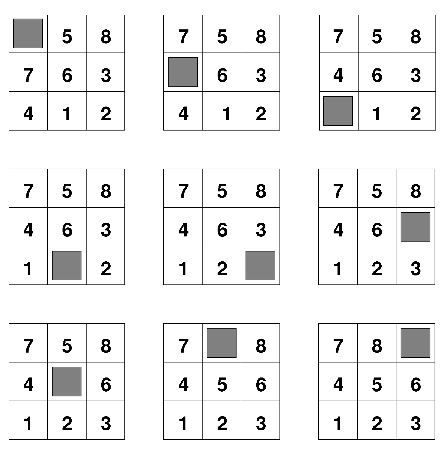
In Figure 1, we see an example representing a sequence of states that leads from the initial configuration to the goal configuration.
Another example consists of the task of building a tower from a collection of blocks [1]. A robot arm can stack, unstack and move the blocks at a table. The production system implements a search algorithm that defines a problem space and can be represented as a tree search.
1.1. Tree Search and the Path Descriptors
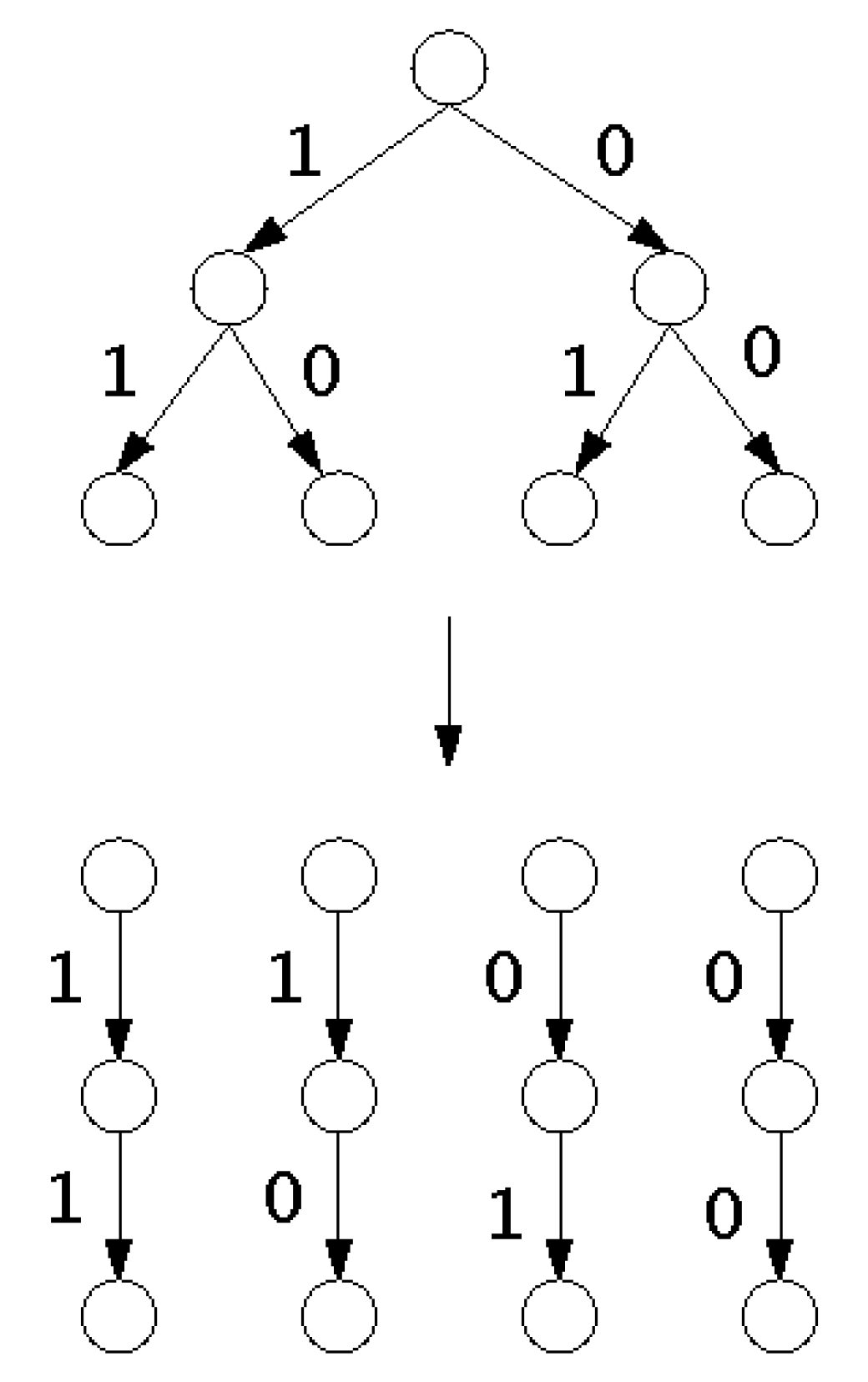
Nodes and edges represent a search tree. Each node represents a state, and each edge represents a transition from one state to the following state. The initial state defines the root of the tree. From each state, either states can be reached, or the state is a leaf. From a leaf, no other state can be reached. B represents the branching factor of the node, the number of possible choices. A leaf represents either the goal of the computation or an impasse when there is no valid transition to a succeeding state. Every node besides the root has a unique node from which it was reached, which is called the parent. Each node and its parent are connected by an edge. Each parent has B children. If , each of the m questions has a reply of either “yes” or “no” and can be represented by a bit (see Figure 2). The m answers are represented by a binary number of length m.
There are possible binary numbers of length m. Each binary number represents a path from the root to a leaf. For each goal, a certain binary number indicates the solution. For a constant branching factor , each question has B possible answers. The m answers can be represented by m digits. For example, with , the number is represented by bits. These numbers represent all paths from the root to the leaves.
1.2. Quantum Tree Search
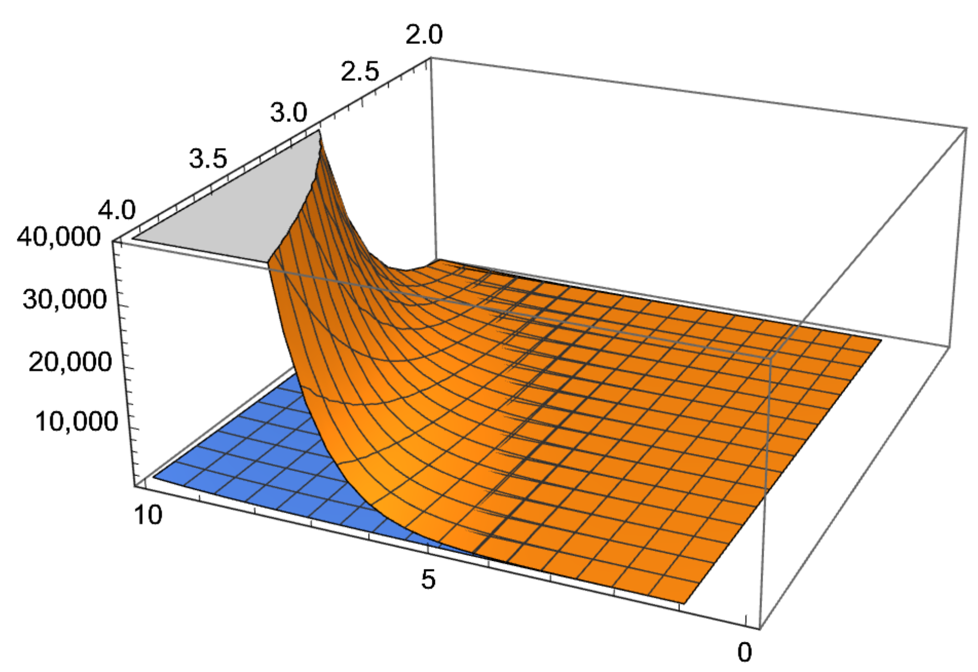
In a quantum computation, we can simultaneously represent all possible path descriptors. There is one path descriptor for each leaf of the tree. Using Grover’s algorithm, we search through all possible paths and verify whether each path leads to the goal state. This type of procedure is called a quantum tree search [5,6]. For possible paths, the costs are (approximately) (see Figure 3).
A constraint of this approach is that we must know the depth m of the search tree in advance. The constraint can be overcome by iterative deepening. In an iterative deepening search. During the iterative deepening search, the states are generated multiple times [7,8]. The time complexity of the iterative deepening search is of the same order of magnitude as a search to the maximum depth [7], as explained by Richard E. Korf: “Since the number of nodes on a given level of the tree grows exponentially with depth, almost all time is spent in the deepest level, even though shallower levels are generated an arithmetically increasing number of times.” The paradox can be explained using the arithmetic–geometric sequence. A quantum iterative deepening search is equivalent to the iterative deepening search [9]. For each limit max, a quantum tree search is performed from the root, where max is the maximum depth of the search tree. The possible solutions are determined using a measurement. We gradually increase the limit of the search from one, to two, three and four and continue to search until the goal is found. For each limit m, a quantum tree search is performed from the root, with m being the maximum depth of the search tree. The possible solutions are determined by a measurement. The time complexity of an iterative deepening search has the same order of magnitude as the quantum tree search. The total costs of m iterations with m measurements are
the equation is based on the geometric series [9].
A second constraint is represented by the constant branching factor. If the branching factor is not constant, the maximal branching factor must be used for the quantum tree search [6].
1.3. Contribution
We present the quantum tree search qiskit implementation by examples from symbolical artificial intelligence, the 3-puzzle, 8-puzzle and the ABC blocks world. Alternative approaches were presented for how to solve the n-puzzle problem by quantum annealing [10,11,12]. Quantum annealing solves optimization problems by finding the global minimum of a function [13,14,15] described by the problem Hamiltonian and the initial Hamiltonian (disordering Hamiltonian). The Hamiltonian describes the configuration of the system by a hilly “surface” [16]. The Hamiltonian always decreases (or remains constant) as the system evolves to its dynamical rule. Attractors are the local minima of the Hamiltonian (energy function). Our implementation is based on the theoretical models of the quantum tree search [6,9]. In these models, the operators are described by permutation matrices of high dimension.
We indicate how the permutation matrices can be efficiently decomposed by quantum gates. The decomposition leads to two principles of symbolical representation. Either the position description (adjective) is fixed and the object descriptor moves (is changed) or, in the reverse interpretation, the object descriptor is fixed and the position descriptor (adjective) moves (is changed). We indicate how to decompose the permutation operator that executes the rules by the two principles.
By simulating the quantum tree search, it becomes clear that the branching factor is reduced by Grover’s amplification to the square root of the average branching factor and not to the maximal branching factor as previously assumed [6].
2. Quantum Tree Search with Qiskit
We explain the principles of quantum tree search by a qiskit quantum production system representing the 3-puzzle. In the next step, we generalize the qiskit description to the 8-puzzle and to block world production systems. Qiskit is an open-source software development kit (SDK) for working with quantum computers at the level of circuits and algorithms. It provides tools for creating and manipulating quantum programs and running them on prototype quantum devices on the IBM Quantum Experience or on simulators on a local computer. It follows the quantum circuit model for universal quantum computation and can be used for any quantum hardware that follows this model.
Qiskt provides different backend simulator functions, in our experiment we use tow simulators.
- The qasm simulator promises to behave like an actual device of today, which is prone to noise resulting from decoherence. It returns counts, which are a sampling of the measured qubits that have to be defined in the circuit, which is much smaller in size and will not increase in size exponentially as the number of qubits increases.
- The statevector simulator performs an ideal execution of qiskit circuits and returns the final state vector off the simulator after application (all qubits). The state vector of the circuit can represent the probability values that correspond to the multiplication of the state vector by the unitary matrix that represents the circuit. The statevector simulator will take longer than other simulation methods and requires more computer memory since the state vector dimension grows exponentially with the number of qubits with (with m number of qubits).
2.1. 3-Puzzle
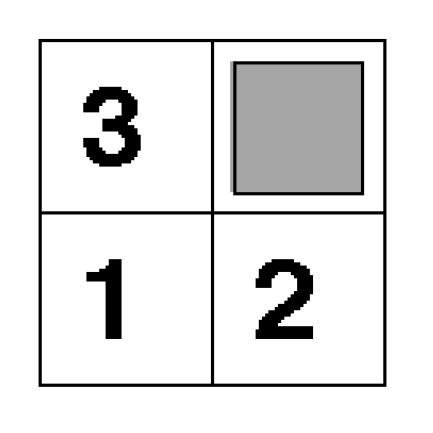
The 3-puzzle is composed of three numbered movable tiles in a frame (see Figure 4).
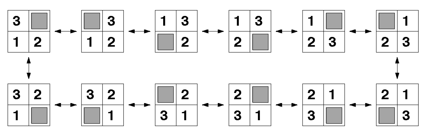
One cell of the frame is empty, and because of this tiles can be moved around to form different patterns [5]. The goal is to find a series of moves of tiles into the blank space that changes the board from the initial configuration to a desired configuration. There are twelve possible configurations (see Figure 5). For any of these configurations, only two movements are possible. The movement of the empty cell is either a clockwise or counter-clockwise movement.
The 3-puzzle is tractable and requires fewer qubits to encode.
There are four different objects: three cells and one empty cell. Each object can be coded by two qubits () and a configuration of the four objects can be represented by a register of eight qubits . In this representation, position description (adjective) is fixed and the class descriptors moves. The control function of the quantum production system needs to fulfill two requirements [17]:
- For a given board, configuration and a production rule determine the new board configuration.
- To determine if the configuration is the goal configuration.
The new board configuration is determined by productions that are represented by the function p. There are four possible positions of the empty cell. The input of the function p is the current board configuration and a bit m that indicates whether the blank cell should perform a clockwise or counter-clockwise movement . Together, there are 8 possible mappings, which are represented by 8 productions. There are four possible positions of the empty cell times two possible moves. For simplicity, we represent the mappings of the function p by a unitary permutation matrix . For each mapping, the empty tile can have three different neighbors. It follows that, in total, there are instantiated rules. They correspond to permutations in the unitary permutation matrix . The matrix acts on the qubits with and
The matrix represents the long-term memory of our production system.
The function , called oracle, determines if the configuration is the goal configuration.
Function oracle is represented by a unitary operator T (for target). T acts on the qubits, with and being the auxiliary qubit
2.1.1. Decomposition of Unitary Operators
An important open question is whether the permutation matrix of dimension can be decomposed. It is possible to determine if a permutation is tensor decomposable and to chose an efficient tensor decomposition if present [5,18]. An alternative less costly representation of the long-term memory can be realized by a uniformly polynomial circuit that describes the function p.
2.1.2. Representation
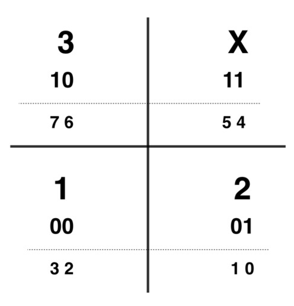
There are four different objects: three cells and one empty cell. Each object can be coded by two qubits (), and a configuration of the four objects can be represented by a register of eight qubits . The object 1 is represented by 00, 2 is represented by 01, 3 is represented by 10 and empty space x is represented by 11. The state is represented by 8 qubits , and the state of the Figure 4 is represented by the qubits , see Figure 6.
In this representation, position description (adjective) is fixed and the class descriptors moves. In the qiskit circuit, all qubits before the computation are in the state 0, so the state of the Figure 6 is prepared with the gate with the following commands of the qubits 0 to 7:
qc.x(0)
qc.x(4)
qc.x(5)
qc.x(7)
In the 3-puzzle task, we have four different rules defined by the position of the empty space. Each of the rules has two instantiations, either moving the empty space clockwise or a counter-clockwise movement. We recognize the four rules and indicate the presence of a rule by a qubit. We use four qubits that indicate the presence of the four rules and call them the trace. We need the trace represented by the four qubits, since we cannot delete the information and we cannot un-compute the output back. By un-computing, we would redo the rules. Additionally, we require a flag represented by a qubit that indicates to us if the rule with the corresponding instantiation can be executed or not. Finally, we need a qubit that represents the path descriptor that will be present by superposition using a Hadamard gate. Altogether, we need fourteen qubits, and we define the following circuit:
qc = QuantumCircuit(14,8)
#State Preparation 0-7
qc.x(0)
qc.x(4)
qc.x(5)
qc.x(7)
#Flag represented by qubit 8
#1St Trace represented by qubits 9-12
#1St Path descriptor in superposition
qc.h(13)
qc.barrier()
defines a quantum circuit with the name that uses 14 qubits and measures 8 qubits.
2.1.3. Rules and Trace
The if part of the rules is implemented by the Toffoli gate, also called the ccX gate (CCNOT gate, controlled controlled not gate), it recognizes the position of the empty space and indicates it by setting one qubit of the four qubits 9 to 11 to one.
#If part of rules marked in trace
qc.ccx(0,1,9)
qc.ccx(2,3,10)
qc.ccx(4,5,11)
qc.ccx(6,7,12)
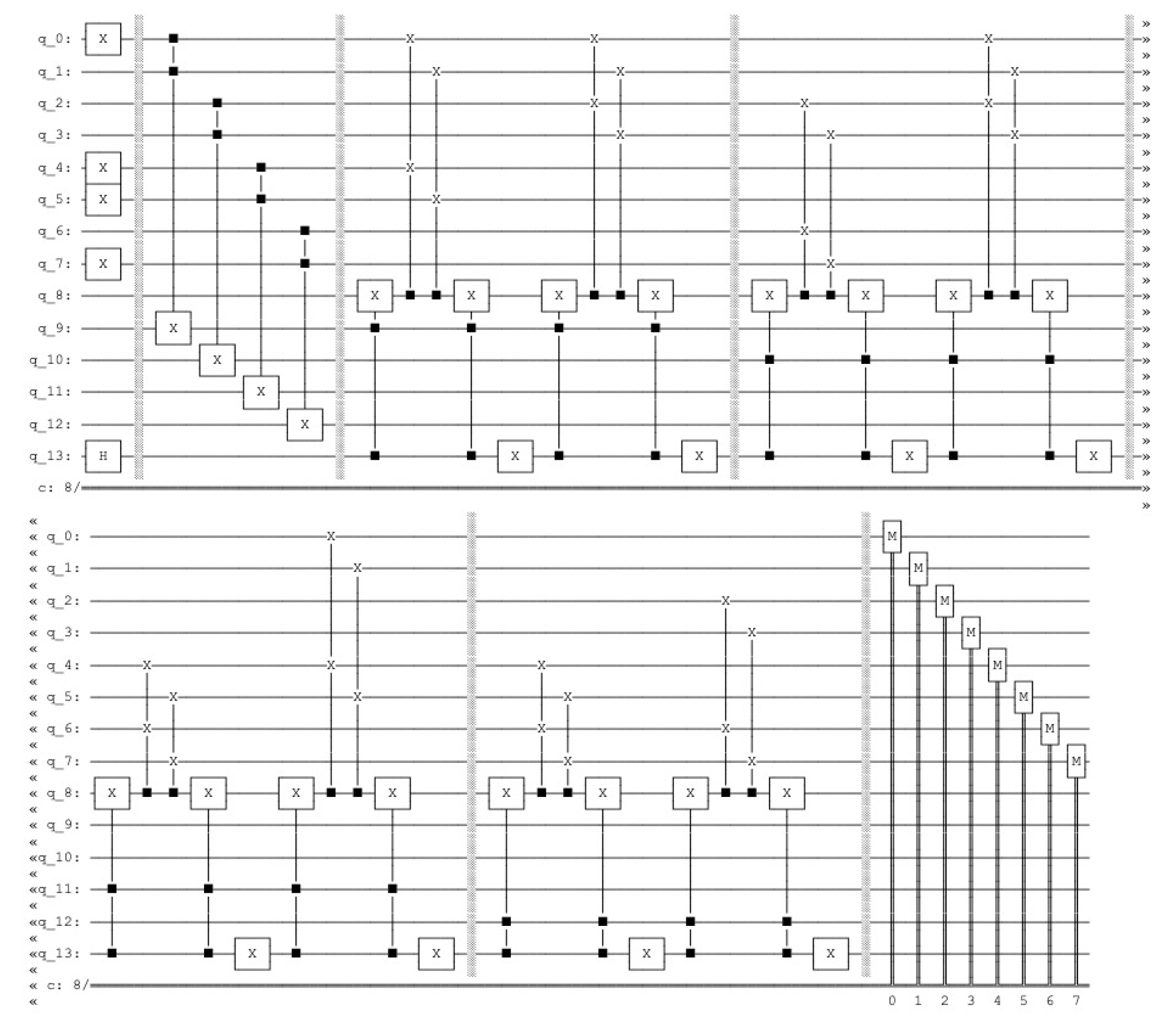
The execution of the rules uses the Fredkin gate, also called controlled swap (CSWAP) gate, using the trace information and the path descriptor setting the flag qubit (qubit 8) to indicate if the rule is going to be executed. The reset is performed by un-computing, by repeating the operation to set the flag again in the state zero. We change the path descriptor by the NOT gate and execute the second instantiation of the rule depending on the trace value; the will separate the representation in the circuit (see the Appendix A.1.1 3-Puzzle Rules), resulting in the quantum circuit indicated in the Figure 7.
By performing the simulation
simulator = Aer.get_backend(’qasm_simulator’)
result=execute(qc,simulator).result()
counts = result.get_counts()
plot_histogram(counts)
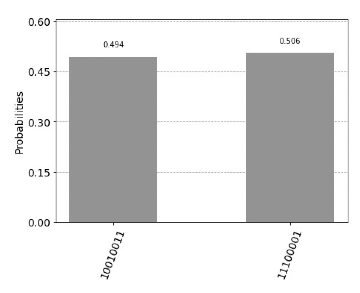
we obtain the following representation of the two generated new states represented by the histogram in the Figure 8.
2.2. Search of Depth Two
Grover’s amplification cannot be applied to fewer than four states. A search of depth one for the 3-puzzle results in two states and a search of depth two in four states. The operator that describes the search of depth two is represented as
using two qubits, , representing the path descriptor. The unitary operator T represents the oracle function that determines if the configuration is the goal configuration
For the function , the solution is encoded by , the sign of the amplitude. If the path descriptor is represented by m qubits, it can represent states. To see why the the solution is encoded by , we indicate the derivative. The auxiliary qubit c is set to one, and the path descriptor is represented by m qubits . First, we set the path descriptor and the auxiliary qubit in superposition by the Hadamard gate for qubits , and then we execute the unitary operator T
There are four possible cases with the path descriptor being the solution:
It follows that
The value of the function is encoded by . We can set the auxiliary qubit to zero by the Hadamard gate. For simplicity, we ignore the trace and the flag qubit and we obtain
The operator that describes the application of the production rules for the 3-puzzle for the depth search t, and a test condition in order to determine if the final board is a target configuration board, is represented with
and
as
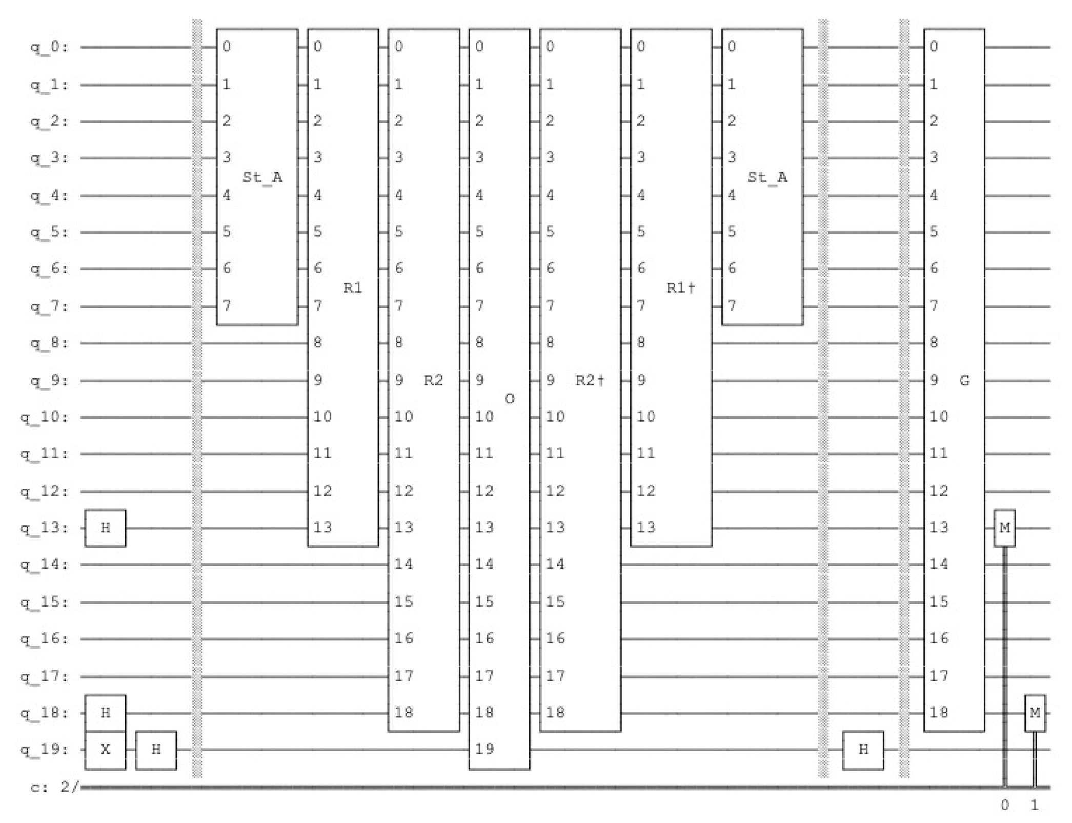
With depth search , an additional four qubits are needed to represent the new trace, one additional qubit for the path descriptor of the depth two and one auxiliary qubit for the oracle operation. The quantum circuit is represented by 20 qubits. We measure the path descriptor represented by two qubits 13 and 18.
qc = QuantumCircuit(20,2)
#State Preparation 0-7
# Flag bit 8
#1St Trace 9-12
#1St Path Descriptor in superposition
qc.h(13)
#1St Trace 14-17
#2th Path Descriptor in superposition
qc.h(18)
#Aux Bit c indicating the solution is negated
# and put in superposition
qc.x(19)
qc.h(19)
In the following, we use the qiskit function to define the oracle using the command. The is a multi-controlled X (Toffoli) gate. A multi-controlled X gate is composed of a simple (Toffoli) gate and temporary work registers. It is represented in the qiskit circuit library.
def oracle():
qc = QuantumCircuit(20)
gate = MCXGate(4)
#Goal Configurations
qc.append(gate,[2, 3, 4, 7, 19])
#Alternative Goal Configurations
#qc.append(gate,[0, 2, 3, 5, 19])
#Grover in depth two cannot resolve this since
two solutions out of four are marked.
#qc.append(gate,[0, 4, 5, 7, 19])
qc.name="O"
return qc
In quantum computation, it is not possible to reset the information to the pattern representing the initial state. Instead, we un-compute the output back to the input before applying the amplification step of the Grover’s algorithm. Because of the unitary evolution, it follows that
the computation can be undone and the corresponding path is marked by a negative sign using the auxiliary qubit c.
We use the qiskit inverse command to perform the inverse operation
def rules1_inv():
qc=rules1()
qc_inv=qc.inverse()
qc_inv.name="R1†"
return qc_inv
The Grover’s amplification is applied to the two qubits, 13 and 16, representing the path descriptor
def Grover():
qc = QuantumCircuit(19)
#Diffusor
qc.h([13,18])
qc.z([13,18])
qc.cz(13,18)
qc.h([13,18])
qc.name="G"
return qc
The quantum circuit using the defined functions is represented in Appendix A.1.2 3-Puzzle Task and indicated in the Figure 9.
2.2.1. Search Depth Three
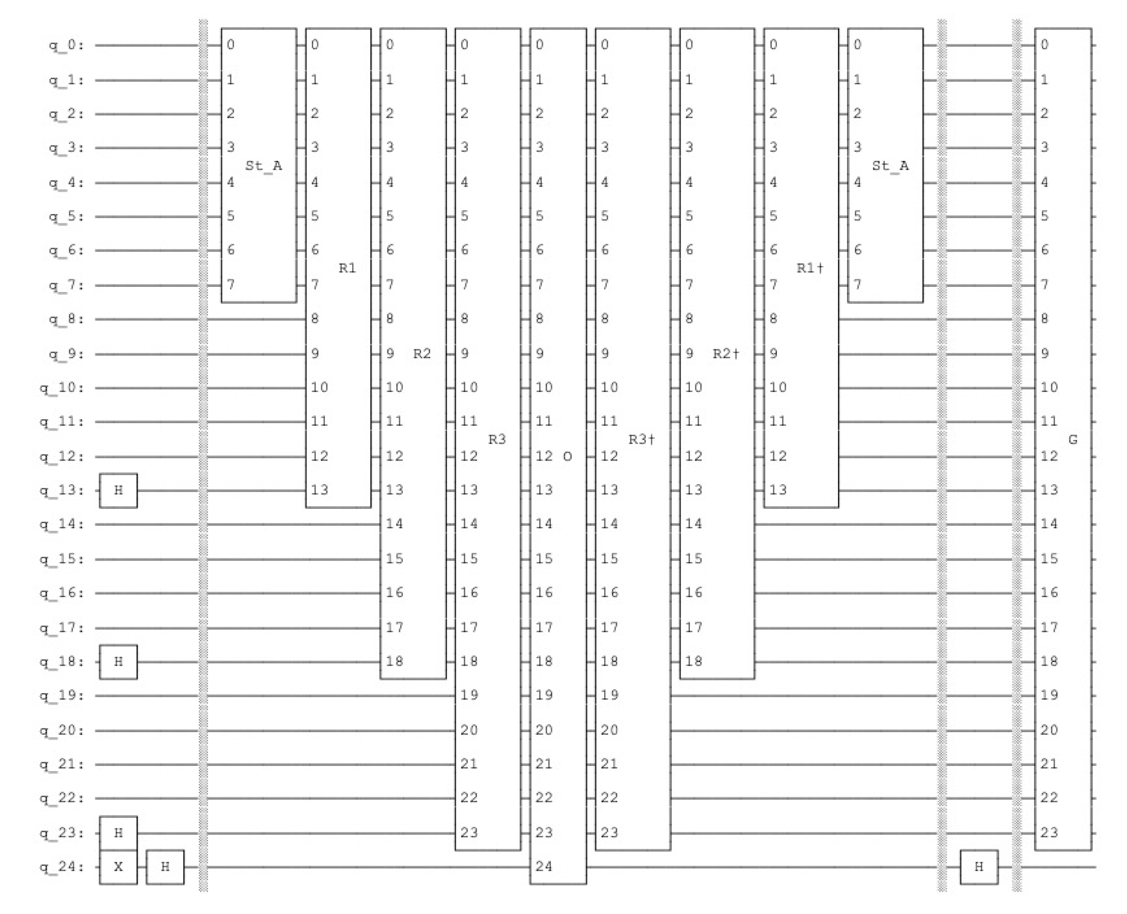
A search of depth three is described by a path descriptor of three qubits. The Grover amplification acts on the qubits 13, 18 and 23 that describe the path descriptor resulting in eight states.
def Grover():
qc = QuantumCircuit(24)
#Diffusor
qc.h([13,18,23])
qc.x([13,18,23])
qc.h(13)
qc.ccx(18,23,13)
qc.h(13)
qc.x([13,18,23])
qc.h([13,18,23])
qc.name="G"
return qc
The circuit is indicated in Figure 10.
The statevector simulator without any measurements represents all probabilities of all qubits.
simulator = Aer.get_backend(’statevector_simulator’)
result=execute(qc,simulator).result()
counts = result.get_counts()
plot_histogram(counts)
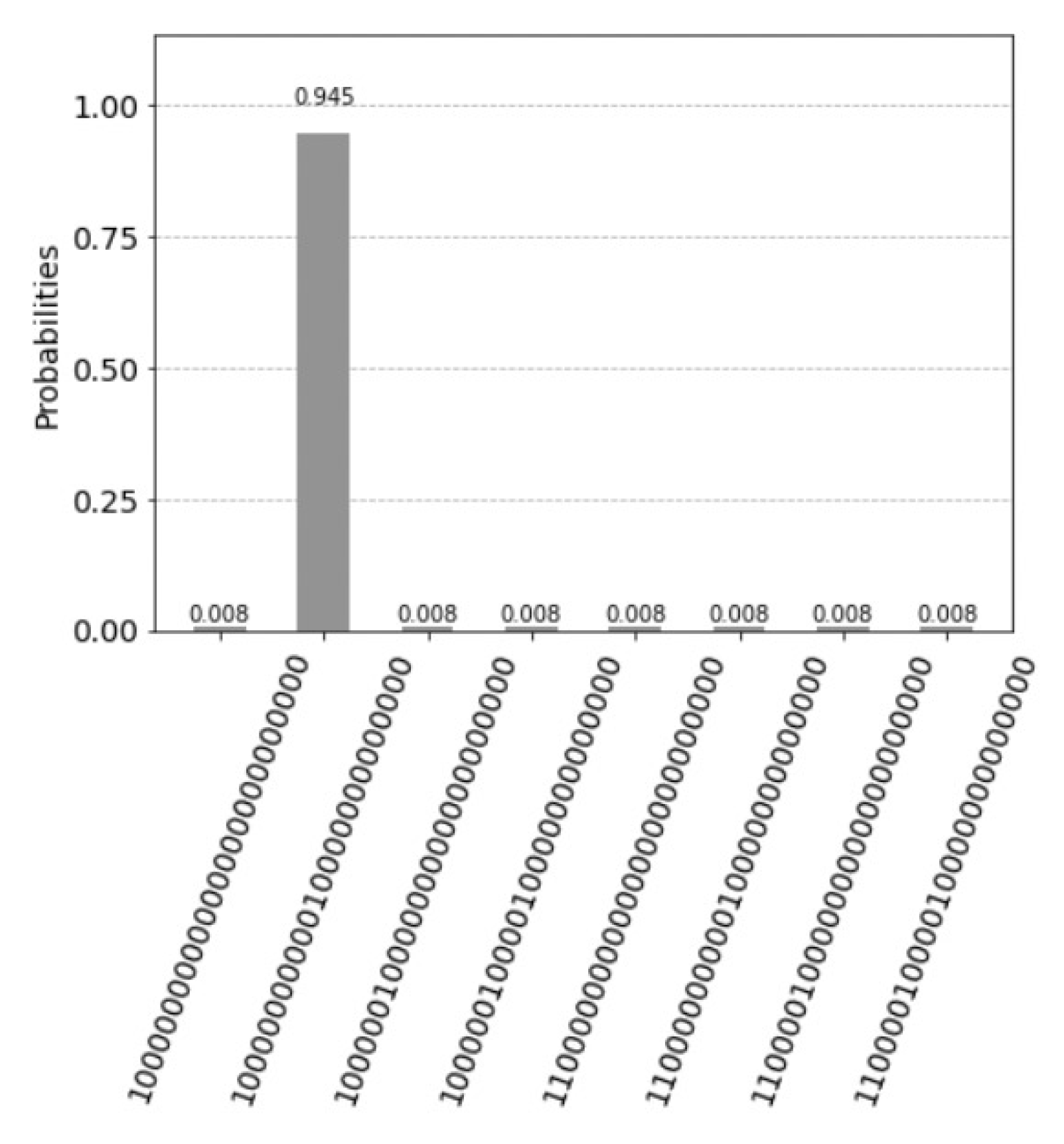
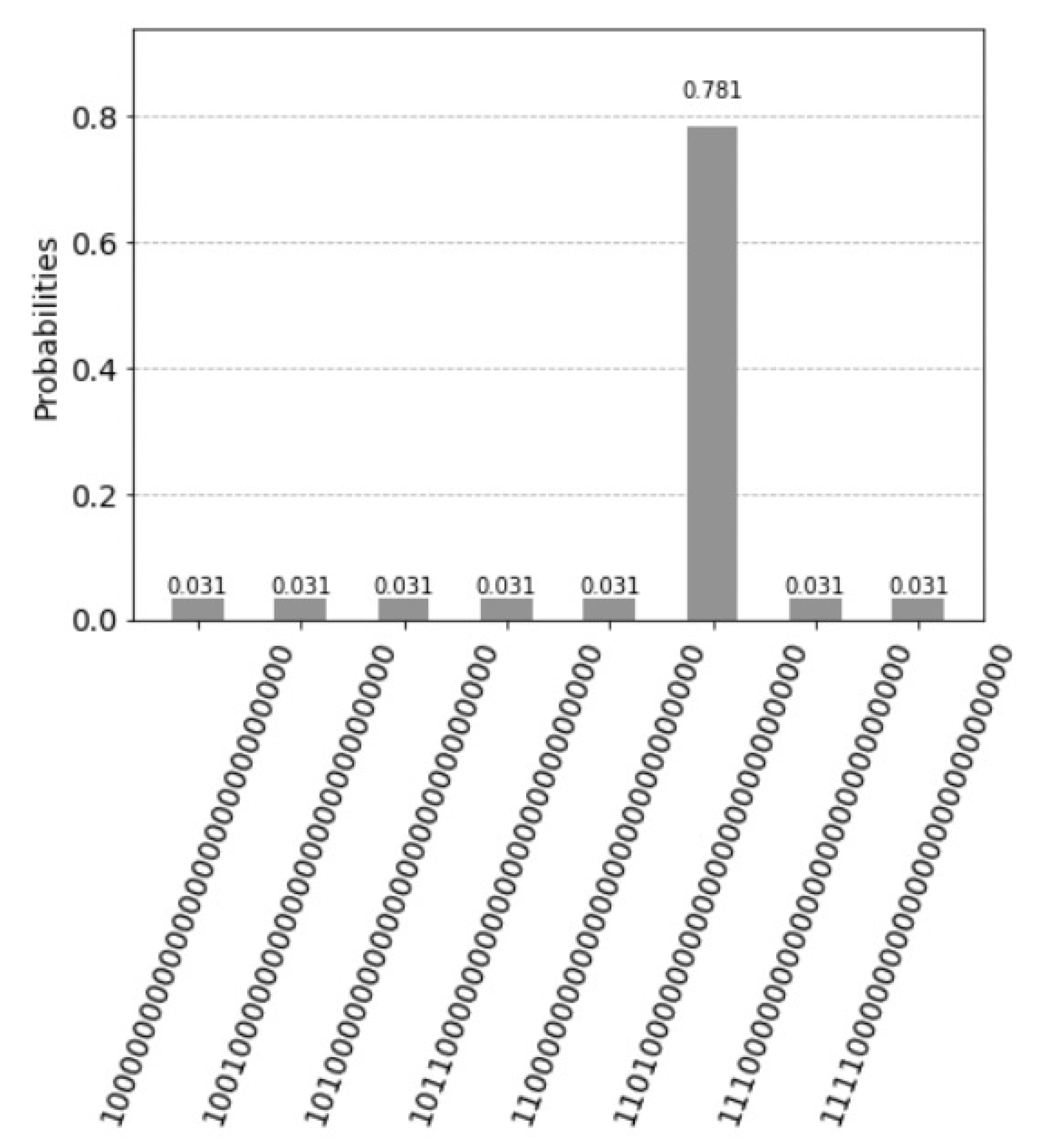
The circuit’s depth in the number of quantum gates is 13. The depth of a circuit is a metric that calculates the longest path between the input data and the output data. The path descriptor has eight possible states represented by three qubits. One marked state results after one iteration is indicated in the histogram of Figure 11. One marked state resulted after one iteration is indicated with a probability value and the path descriptor 001. The path descriptor can be verified by measurement using the qasm simulator as well.
2.2.2. Search Depth Three with Two Iterations
We apply the operator ignoring the trace for simplicity for the depth t resulting in states represented by the path descriptor
With Grover amplification on t qubits representing the path descriptor by the unitary operator
With r iterations
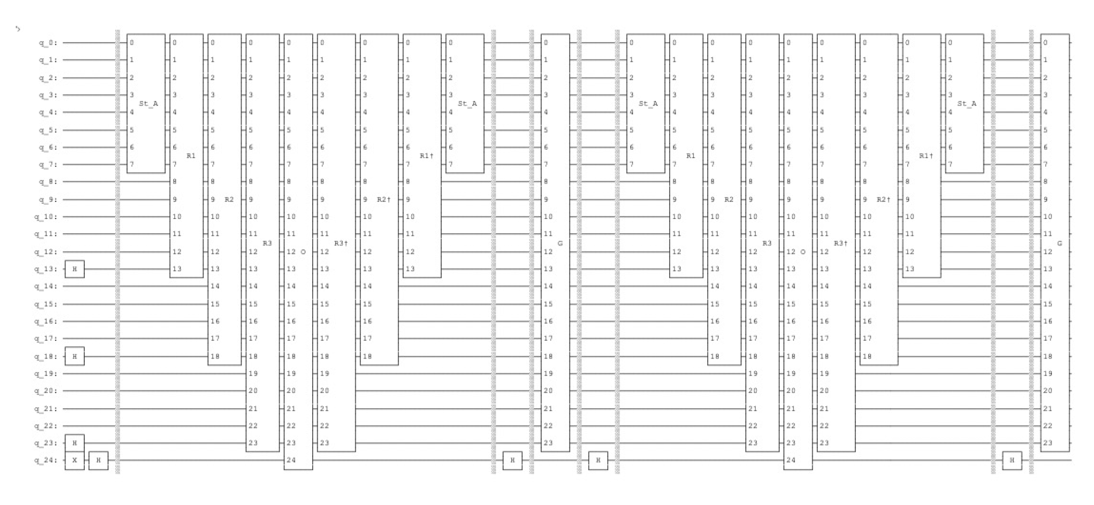
and determine the solution by the measurement of the register that represents the path descriptor. In our case and , with resulting in the circuit represented in the Figure 12. One marked state results after two iterations are indicated in the histogram of Figure 13. One marked state results after two iterations are indicated with a probability value of and the path descriptor 001.
The 3-puzzle quantum production system highlighted the principles of quantum tree search and quantum production systems. It does not give any true computational speed up due to the simplicity of the problem.
3. Extending to 8-Puzzle
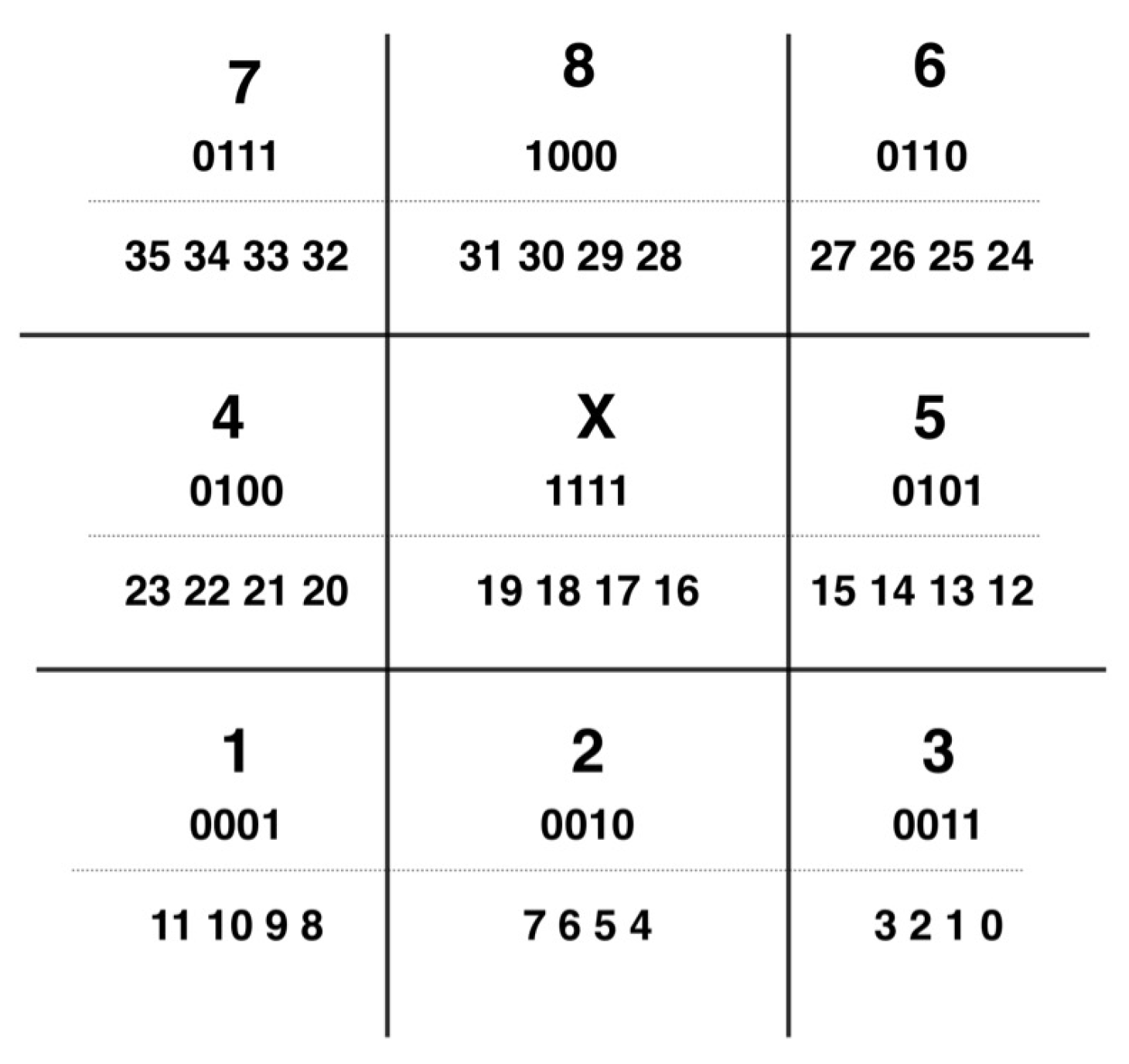
For 8-puzzle, there are 9 different objects: eight cells and one empty cell. Each object has to be represented by four 4 qubits since 3 qubits allow only to represent different states. The object 1 is represented by 001, 2 is represented by 010 and 3 is represented by 011, and we continue the representation as binary numbers with 8 represented as 1000. We represent the empty space x by 1111. The state is represented by 36 qubits , see Figure 14.
The empty cell can be present in 9 different positions. The empty cell can move either up, down, left or right. The new board configuration is determined by the function p. The input of the function p is the current board configuration and two bits (qubits 46 and 47) indicating whether the blank cell should perform move right , left , up or down . There are 36 qubits to represent the state and 9 qubits for the trace, together with the auxiliary qubit 49 qubits are represented by the quantum circuit.
qc = QuantumCircuit(49,2)
#State Preparation 0-35
#N3
qc.x(0)
qc.x(1)
#2
#3
..
..
#Flag 36
#1St Trace 37-45
#1St Path Descriptor in superposition 46, 47
qc.h(46)
qc.h(47)
#Preparation of Aux
qc.x(48)
qc.h(48)
In case the empty cell is in the center, four movements are possible. For a cell in the edge, only three movements are possible, for the corner, only two movements are possible
def if_rules():
qc = QuantumCircuit(46)
#Marke the trace indicate the rule group through trace
gate = MCXGate(4)
#Empty Space in corner, 2 movements
qc.append(gate, [0, 1, 2, 3, 37])
#Empty Space in edge, 3 movements
qc.append(gate, [4, 5, 6, 7, 38])
#Empty Space in corner, 2 movements
qc.append(gate, [8, 9, 10, 11, 39])
#Empty Space in edge, 3 movements
qc.append(gate, [12, 13, 14, 15, 40])
#Empty Space in center, 4 movements
qc.append(gate, [16, 17, 18, 19, 41])
#Empty Space in edge, 3 movements
qc.append(gate, [20, 21, 22, 23, 42])
#Empty Space in corner, 2 movements
qc.append(gate, [24, 25, 26, 27, 43])
#Empty Space in edge, 3 movements
qc.append(gate, [28, 29, 30, 31, 44])
#Empty Space in corner, 2 movements
qc.append(gate, [32, 33, 34, 35, 45])
qc.name="IF"
return qc
For the empty space in the center, there are four instantiations corresponding to the four movements
- For the path descriptor 00, move right .
- For the path descriptor 00, move left .
- For the path descriptor 00, move up .
- For the path descriptor 00, move down .
See Appendix A.2.1 Puzzle Rules1 8-Puzzle. For the empty space in the edge, there are four instantiations corresponding to the three movements. The representation if performed in the same way as before, in our example, the empty space is at the position .
- For the path descriptor 00, move up .
- For the path descriptor 01, move down .
- For the path descriptor 10, move left .
- For the path descriptor 11, move left .
The only difference is that the rule move left is repeated twice. For the empty space in the corner, there are four instantiations corresponding to the two movements. The representation is performed in the same way as before, in our example, the empty space is at the position .
- For the path descriptor 00, move up .
- For the path descriptor 01, move up .
- For the path descriptor 10, move left .
- For the path descriptor 11, move left .
The rule move left and the rule move left are repeated twice. Simulating 36 qubits requires higher memory capacity, we cannot use the statevector simulator or a search depth of two due to memory constraints. We can measure the path descriptor after applying the function rules1 8 puzzle, see Figure 15. These constraints can be overcome by higher memory capacity.
Number of Iterations
For 8-puzzle , and
Naïvely, we would assume that the branching factor is reduced by Grover’s amplification to
However, this is not the case in our coding strategy. With growing value n, the branching factor is reduced by Grover’s amplification to
For k solutions, the probability of measuring a state that represents one solution of k solutions is related to the number r of iterations of the Grover’s operator. The probability of seeing one solution should be as close as possible to 1, and the number of iterations r should be as small as possible. After r iterations, the probability of measuring a solution is nearly one, with m being the number of qubits describing the path descriptor [19,20]
The number of iterations r is the largest integer not greater than the computed value. Simplified, we can state that
The value of r depends on the relation of m versus k. For the depth m, there are k solutions with
it follows
and the branching factor is reduced by Grover’s amplification to
4. Blocks World
The blocks world is a planning domain in artificial intelligence [1]. The blocks can be placed at the table and picked up and set down on a table or another block, and the goal is to build one or more vertical stacks of blocks. Only one block may be moved at a time and any blocks that are under another block cannot be moved. There are three different types of blocks. They differ by attributes such as color (red, green and blue) or marks, but not by form. In AI, they are traditionally called A, B, C blocks [4].
4.1. Representation
The class descriptor is fixed and the position descriptor (adjective) moves. It is reversed as in the puzzle examples, since the reverse in this case is a more economic representation requiring 9 qubits, three qubits for each block (see Figure 16 and Figure 17).
The architecture uses 27 qubits, 9 for representation of the state, one for flag and 13 qubits to represent the 13 different categories of rules. The path descriptor for the depth search one is represented by three qubits, since the number of maximal instantiations is six.
qc = QuantumCircuit(27)
#State Preparation 0-8
# Flag 9
#1st Trace (ten) 10-22 Rule Classes
#1st Path descriptor represented by three qubit
qc.h(23)
qc.h(24)
qc.h(25)
#Preparation of Aux
qc.x(26)
qc.h(26)
The architecture is indicated in the Figure 18.
All blocks on the floor are represented as:
ef state_floor():
qc = QuantumCircuit(9)
#All Blocks are on floor
#BLOCK A qubits 0-2
qc.x(2)
#BLOCK B qubits 3-5
qc.x(5)
#BLOCK C qubits 6-8
qc.x(8)
qc.name="S_FL"
return qc
Different classes of rules are recognized during the function. The class all blocks on the floor has one combination (see Figure 19), the class tower appears in six different combinations (see Figure 20) as well as the class small tower and a block on table (such as tower and block A, see Figure 21).
def if_rules():
qc = QuantumCircuit(23)
gate = MCXGate(3)
#All blocks on table
qc.append(gate, [2, 5, 8, 10])
#ABC tower
qc.append(gate, [1, 2, 3, 11])
#ACB tower
qc.append(gate, [1, 2, 6, 12])
#BAC tower
qc.append(gate, [4, 5, 1, 13])
#BCA tower
qc.append(gate, [4, 5, 6, 14])
#CAB tower
qc.append(gate, [1, 7, 8, 15])
#CBA tower
qc.append(gate, [4, 7, 8, 16])
#BC tower and block A
qc.append(gate, [2, 5, 3, 17])
#BA tower and block C
qc.append(gate, [8, 5, 3, 18])
#CA tower and block B
qc.append(gate, [8, 6, 5, 19])
#CB tower and block A
qc.append(gate, [8, 6, 2, 20])
#AC tower and block B
qc.append(gate, [0, 2, 5, 21])
#AB tower and block C
qc.append(gate, [0, 2, 8, 22])
qc.name="IF"
return qc
The class tower, such as for example the tower, has just one instantiation; the class small tower and a block on the table (such as tower and block A) have three instantiations. All blocks on the table have six different instantiations, for each block, there are two rules, see the Appendix A.3.1 for the qiskit listing for rules floor.
The class tower (such as for example the tower) appears in six different combinations. For each combination, there is only one instantiation that is represented through all eight states:
def rules_tw():
qc = QuantumCircuit(17)
#There is a tower,
#6 different towers indicated by 11,12,..,16
qc.cswap(11,1,5)
qc.cswap(12,1,8)
qc.cswap(13,2,4)
qc.cswap(14,2,8)
qc.cswap(15,2,7)
qc.cswap(16,5,7)
qc.name="R_TW"
return qc
There are six combinations of the class small tower and a block on the table (such as tower and block A). Each of these combination has three instantiations. Since there are eight possible states represented by the path descriptor for each combination, the three instantiations are executed twice with two additional instantiations. See Appendix A.3.2 for the qiskit listing for rules tw bl.
4.2. Number of Iterations
For A, B, C blocks , and
Naïvely, we would assume that the branching factor is reduced by Grover’s amplification to the number 8 represented by three qubits
With growing value m, the branching factor is reduced by Grover’s amplification to
For k solutions, the probability of measuring a state that represents one solution of k solutions is related to the number r of iterations of the Grover’s operator. Simplified, we can state that
The value of r depends on the relation of m versus k. For the depth m
it follows
and the branching factor is reduced by Grover’s amplification to .
5. Conclusions
The objects are represented by symbols and adjectives. The object is always present in the world and only its adjectives, such as the position value, change by permutations. Two principles of representations were presented. Either the position description (adjective) is fixed and the class descriptors moves/is changed or, in the reverse interpretation, the class descriptor is fixed and the position descriptor (adjective) moves/is changed. Depending on the task, one representation of the two is more economic than the other. We have shown by three examples how to implement a quantum tree search algorithm using qiskit using simulation. The efficient implementation is based on the state representation and the trace that allows a deeper search. We have shown as well that the branching factor is reduced by Grover’s amplification to the square root of the average branching factor.
Funding
This work was supported by national funds through FCT, Fundação para a Ciência e a Tecnologia, under project UIDB/50021/2020.
Institutional Review Board Statement
This article does not contain any studies with human participants or animals performed by any of the authors.
Informed Consent Statement
Not applicable.
Data Availability Statement
The datasets used in this paper are provided within the main body of the manuscript.
Conflicts of Interest
The author declares no conflict of interest.The funders had no role in study design, data collection and analysis, decision to publish, or preparation of the manuscript.
Appendix A. Qiskit Code
Appendix A.1. 3-Puzzle
Appendix A.1.1. 3-Puzzle Rules
#If then rule (1) for empty at 0, 1 -> 4, 5 or 2, 3
#Search empty state with the descriptor
qc.ccx(9,13,8)
#Execute 1st then part by moving the empty space clockwise
qc.cswap(8,0,4)
qc.cswap(8,1,5)
#Secod then part with changed descriptor
#Reset Flag
qc.ccx(9,13,8)
#Fetch second superposition
qc.x(13)
qc.ccx(9,13,8)
#Execute 2th then part by moving the empty space anti-clockwise
qc.cswap(8,0,2)
qc.cswap(8,1,3)
#Reset Flag
qc.ccx(9,13,8)
#Restore descriptor
qc.x(13)
qc.barrier()
The second rule is represented accordingly.
#If then rule (2) for empty at 2, 3 -> 6, 7 or 0, 1
#Search empty state with the descriptor
qc.ccx(10,13,8)
#Execute 1st then part
qc.cswap(8,2,6)
qc.cswap(8,3,7)
#Secod then part with changed descriptor
#Reset Flag
qc.ccx(10,13,8)
#Fetch second superposition
qc.x(13)
qc.ccx(10,13,8)
#Execute 2th then part
qc.cswap(8,0,2)
qc.cswap(8,1,3)
#Reset Flag
qc.ccx(10,13,8)
#Restore descriptor
qc.x(13)
qc.barrier()
The third and the fourth rules are represented in the same way. Finally, we measure the state represented by the 8 qubits.
qc.measure(0,0)
qc.measure(1,1)
qc.measure(2,2)
qc.measure(3,3)
qc.measure(4,4)
qc.measure(5,5)
qc.measure(6,6)
qc.measure(7,7)
Appendix A.1.2. 3-Puzzle Task
qc = QuantumCircuit(20,2)
#State Preparation 0-7
# Flag bit 8
#1St Trace 9-12
#1St Path Descriptor in superposition
qc.h(13)
#1St Trace 14-17
#2th Path descriptor in superposition
qc.h(18)
#Aux bit c indicating the solution is negated and
# put in superposition
qc.x(19)
qc.h(19)
qc.barrier()
#Preperation of state
qc.append(state_A(),range(8))
#Depth1
qc.append(rules1(),range(14))
#Depth2
qc.append(rules2(),range(19))
#Oracle
qc.append(oracle(),range(20))
#Depth2
qc.append(rules2_inv(),range(19))
#Depth1
qc.append(rules1_inv(),range(14))
#Redo Preperation
qc.append(state_A(),range(8))
qc.barrier()
#Redo Superposition of Aux Bit
qc.h(19)
qc.barrier()
qc.append(Grover(),range(19))
qc.measure(13,0)
qc.measure(18,1)
Appendix A.2. 8-Puzzle
Appendix A.2.1. Rules1 8-Puzzle
def rules1():
qc = QuantumCircuit(48)
#Flag 36
#Path Descriptor 46, 47
#Trace 37-45
flag_gate = MCXGate(3)
#If then rule move right, for~empty at 16, 17, 18, 19 -> 12, 13, 14, 15
qc.append(flag_gate, [41, 46, 47, 36])
#Move
qc.cswap(36,16,12)
qc.cswap(36,17,13)
qc.cswap(36,18,14)
qc.cswap(36,19,15)
#Clear Flag
qc.append(flag_gate, [41, 46, 47, 36])
#If then rule move left, for~empty at 16, 17, 18, 19 -> 20, 21, 22, 23
qc.x(46)
qc.append(flag_gate, [41, 46, 47, 36])
#Move
qc.cswap(36,16,20)
qc.cswap(36,17,21)
qc.cswap(36,18,22)
qc.cswap(36,19,23)
#Clear Flag
qc.append(flag_gate, [41, 46, 47, 36])
qc.x(46)
#If then rule move up, for~empty at 16, 17, 18, 19 -> 28, 29, 30, 31
qc.x(47)
qc.append(flag_gate, [41, 46, 47, 36])
#Move
qc.cswap(36,16,28)
qc.cswap(36,17,29)
qc.cswap(36,18,30)
qc.cswap(36,19,31)
#Clear Flag
qc.append(flag_gate, [41, 46, 47, 36])
qc.x(47)
#If then rule move down, for~empty at 16, 17, 18, 19 -> 4, 5, 6, 7
qc.x(46)
qc.x(47)
qc.append(flag_gate, [41, 46, 47, 36])
#Move
qc.cswap(36,16,4)
qc.cswap(36,17,5)
qc.cswap(36,18,6)
qc.cswap(36,19,7)
#Clear Flag
qc.append(flag_gate, [41, 46, 47, 36])
qc.x(47)
qc.x(46)
qc.name="R1"
return qc
Appendix A.3. ABC Blocks World
Appendix A.3.1. Rules Floor
def rules_floor():
qc = QuantumCircuit(26)
gate4 = MCXGate(4)
qc.append(gate4, [10, 23, 24, 25, 9])
#All blocks on~floor
# Moving A
#A on B
qc.cswap(9,0,5)
#Secod then part with changed descriptor
#Reset WM (Working Memory)
qc.append(gate4, [10, 23, 24, 25, 9])
#Fetch second superposition
qc.x(23)
qc.append(gate4, [10, 23, 24, 25, 9])
#A on C
qc.cswap(9,0,8)
#Reset WM
qc.append(gate4, [10, 23, 24, 25, 9])
#Restore descriptor
qc.x(23)
# Moving B
qc.x(24)
qc.append(gate4, [10, 23, 24, 25, 9])
# B on A
qc.cswap(9,2,3)
#Secod then part with changed descriptor
#Reset WM
qc.append(gate4, [10, 23, 24, 25, 9])
qc.x(24)
#Fetch second superposition
qc.x(23)
qc.x(24)
qc.append(gate4, [10, 23, 24, 25, 9])
#B on C
qc.cswap(9,3,8)
#Reset WM
qc.append(gate4, [10, 23, 24, 25, 9])
#Restore descriptor
qc.x(24)
qc.x(23)
# Moving C
qc.x(25)
qc.append(gate4, [10, 23, 24, 25, 9])
#C on A
qc.cswap(9,6,2)
#Secod then part with changed descriptor
#Reset WM
qc.append(gate4, [10, 23, 24, 25, 9])
qc.x(25)
#Fetch second superposition
qc.x(25)
qc.x(23)
qc.append(gate4, [10, 23, 24, 25, 9])
# C on B
qc.cswap(9,6,5)
#Reset WM
qc.append(gate4, [10, 23, 24, 25, 9])
#Restore descriptor
qc.x(23)
qc.x(25)
#We have only six rules, but~eight possible paths!!!
#To get rid of the initial state we will move C again!!!
# Moving C Again
qc.x(24)
qc.x(25)
qc.append(gate4, [10, 23, 24, 25, 9])
# A clear goes to high of B
qc.cswap(9,6,2)
#Secod then part with changed descriptor
#Reset WM
qc.append(gate4, [10, 23, 24, 25, 9])
qc.x(25)
qc.x(24)
#Fetch second superposition
qc.x(23)
qc.x(24)
qc.x(25)
qc.append(gate4, [10, 23, 24, 25, 9])
# C clear goes to high of B
qc.cswap(9,6,5)
#Reset WM
qc.append(gate4, [10, 23, 24, 25, 9])
#Restore descriptor
qc.x(25)
qc.x(24)
qc.x(23)
qc.name="R_FL"
return qc
Appendix A.3.2. Rules tw bl
def rules_tw_bl():
qc = QuantumCircuit(26)
gate4 = MCXGate(4)
#Flag 9
#Path Descriptor 23, 24, 25
#The three instantiations
#BC tower and block A
#qc.append(gate, [2, 5, 3, 17])
#Put it on Floor
qc.append(gate4, [17, 23, 24, 25, 9])
qc.cswap(9,3,8)
#Clear WM
qc.append(gate4, [17, 23, 24, 25, 9])
#Make Tower BCA
qc.x(23)
qc.append(gate4, [17, 23, 24, 25, 9])
qc.cswap(9,5,1)
#Clear WM
qc.append(gate4, [17, 23, 24, 25, 9])
qc.x(23)
#Move C on the other block A
qc.x(24)
qc.append(gate4, [17, 23, 24, 25, 9])
qc.cswap(9,2,8)
#Clear WM
qc.append(gate4, [17, 23, 24, 25, 9])
qc.x(24)
#Repeat three instantiations again for the states 4-6
# of the path descriptor
#Put it on Floor
qc.x(24)
qc.x(23)
qc.append(gate4, [17, 23, 24, 25, 9])
qc.cswap(9,3,8)
#Clear WM
qc.append(gate4, [17, 23, 24, 25, 9])
qc.x(24)
qc.x(23)
#Make Tower BCA
qc.x(25)
qc.append(gate4, [17, 23, 24, 25, 9])
qc.cswap(9,5,1)
#Clear WM
qc.append(gate4, [17, 23, 24, 25, 9])
qc.x(25)
#Move C on the other block A
qc.x(25)
qc.x(23)
qc.append(gate4, [17, 23, 24, 25, 9])
qc.cswap(9,2,8)
#Clear WM
qc.append(gate4, [17, 23, 24, 25, 9])
qc.x(25)
qc.x(23)
#Repeat two instantiations again for the states 7-8
# of the path descriptor
#Make Tower BCA
qc.x(25)
qc.x(24)
qc.append(gate4, [17, 23, 24, 25, 9])
qc.cswap(9,5,1)
#Clear WM
qc.append(gate4, [17, 23, 24, 25, 9])
qc.x(25)
qc.x(24)
#Move C on the other block A
qc.x(25)
qc.x(24)
qc.x(23)
qc.append(gate4, [17, 23, 24, 25, 9])
qc.cswap(9,2,8)
#Clear WM
qc.append(gate4, [17, 23, 24, 25, 9])
qc.x(25)
qc.x(24)
qc.x(23)
#In the same way
#BA tower and block C
#CA tower and block B
#CB tower and block A
#AC tower and block B
#AB tower and block C
.....
qc.name="R_TB"
return qc
References
- Nilsson, N.J. Principles of Artificial Intelligence; Springer: Berlin/Heidelberg, Germany, 1982. [Google Scholar]
- Anderson, J.R. Cognitive Psychology and Its Implications, 4th ed.; W. H. Freeman and Company: New York, NY, USA, 1995. [Google Scholar]
- Brownston, L.; Farell, R.; Kant, E.; Martin, N. Programming Expert Systems in OPS5: An Introduction to Rule-Based Programming; Addison-Wesley: Boston, MA, USA, 1985. [Google Scholar]
- Luger, G.F.; Stubblefield, W.A. Artificial Intelligence, Structures and Strategies for Complex Problem Solving, 3rd ed.; Addison-Wesley: Boston, MA, USA, 1998. [Google Scholar]
- Wichert, A. Principles of Quantum Artificial Intelligence: Quantum Problem Solving and Machine Learning, 2nd ed.; World Scientific: Porto Salvo, Portugal, 2020. [Google Scholar]
- Tarrataca, L.; Wichert, A. Tree search and quantum computation. Quantum Inf. Process. 2011, 10, 475–500. [Google Scholar] [CrossRef]
- Korf, R.E. Depth-first iterative-deepening: An optimal admissible tree search. Artif. Intell. 1985, 27, 97–109. [Google Scholar] [CrossRef]
- Russell, S.; Norvig, P. Artificial Intelligence: A Modern Approach; Prentice Hall Series in Artificial Intelligence; Prentice Hall: Hoboken, NJ, USA, 2010. [Google Scholar]
- Tarrataca, L.; Wichert, A. Quantum iterative deepening with an application to the halting problem. PLoS ONE 2013, 8, e57309. [Google Scholar]
- Eagle, A.; Kato, T.; Minato, Y. Solving tiling puzzles with quantum annealing. arXiv 2019, arXiv:1904.01770v1. [Google Scholar]
- Hamze, F.; Jacob, D.C.; Ochoa, A.J.; Perera, D.; Wang, W.; Katzgrabe, H.G. From near to eternity: Spin-glass planting, tiling puzzles, and constraint satisfaction problems. arXiv 2018, arXiv:1711.04083v2. [Google Scholar] [CrossRef] [PubMed]
- Takabatake, K.; Yanagisawa, K.; Akiyama, Y. Solving generalized polyomino puzzles using the ising model. Entropy 2022, 24, 354. [Google Scholar] [CrossRef] [PubMed]
- Brooke, J.; Bitko, D.; Rosenbaum, T.; Aeppli, G. Quantum annealing of a disordered magnet. Science 1999, 284, 779–781. [Google Scholar] [CrossRef] [PubMed]
- Johnson, M.W.; Amin, M.H.S.; Gildert, S.; Lanting, T.; Hamze, F.; Dickson, N.; Harris, R.; Berkley, A.J.; Johansson, J.; Bunyk, P.; et al. Quantum annealing with manufactured spins. Nature 2011, 473, 194–198. [Google Scholar] [CrossRef] [PubMed]
- McGeoch, C.C. Adiabatic Quantum Computation and Quantum Annealing: Theory and Practice; Morgan & Claypool: San Rafael, CA, USA, 2014. [Google Scholar]
- Hertz, J.; Krogh, A.; Palmer, R.G. Introduction to the Theory of Neural Computation; Addison-Wesley: Boston, MA, USA, 1991. [Google Scholar]
- Tarrataca, L.; Wichert, A. Problem-solving and quantum computation. Cogn. Comput. 2011, 3, 510–524. [Google Scholar] [CrossRef]
- Kolda, T.G.; Bader, B.W. Tensor decompositions and applications. SIAM Rev. 2009, 51, 455–500. [Google Scholar] [CrossRef]
- Hirvensalo, M. Quantum Computing; Springer: Berlin/Heidelberg, Germany, 2004. [Google Scholar]
- Nielsen, M.A.; Chuang, I.L. Quantum Computation and Quantum Information; Cambridge University Press: Cambridge, MA, USA, 2000. [Google Scholar]
Figure 1.
The first pattern (upper left) represents the initial configuration and the last (low right) the goal configuration. The series of moves describe the solution to the problem.
Figure 1.
The first pattern (upper left) represents the initial configuration and the last (low right) the goal configuration. The series of moves describe the solution to the problem.

Figure 2.
Search tree for and . Each question can be represented by a bit. Each binary number (11, 10, 01, 00) represents a path from the root to the leaf.
Figure 2.
Search tree for and . Each question can be represented by a bit. Each binary number (11, 10, 01, 00) represents a path from the root to the leaf.

Figure 3.
For branching, factor B from 2 to 4 and the depth of the tree search m from 1 to 10. The costs on a conventional computer are , upper plane. On a quantum computer, we need only steps, plane below.
Figure 3.
For branching, factor B from 2 to 4 and the depth of the tree search m from 1 to 10. The costs on a conventional computer are , upper plane. On a quantum computer, we need only steps, plane below.

Figure 4.
The desired configuration of the 3-puzzle.

Figure 5.
There are twelve possible configurations. For any of these configurations, only two movements are possible. The movement of the empty cell is either a clockwise or counter-clockwise movement.
Figure 5.
There are twelve possible configurations. For any of these configurations, only two movements are possible. The movement of the empty cell is either a clockwise or counter-clockwise movement.

Figure 6.
3-puzzle coding representing the state of the Figure 4. The four objects are by a register of eight qubits. We indicate the state, its representation and below the position of the 8 qubits. In this representation, position description (adjective) is fixed and the class descriptors moves.
Figure 6.
3-puzzle coding representing the state of the Figure 4. The four objects are by a register of eight qubits. We indicate the state, its representation and below the position of the 8 qubits. In this representation, position description (adjective) is fixed and the class descriptors moves.

Figure 7.
Quantum circuit representing the generation of two instantiations of rules in the 3-puzzle task of one depth search.
Figure 7.
Quantum circuit representing the generation of two instantiations of rules in the 3-puzzle task of one depth search.

Figure 8.
Two generated new states represented by eight qubits using the qasm simulator.

Figure 9.
The quantum circuit of 3-puzzle task of the depth search 2. The circuits depth in the number of quantum gates is 12. The path descriptor has four possible states represented by two qubits. One marked state results in a certain solution 01 off the path descriptor by the qasm simulator after one iteration, since for one marked qubit one requires only one rotation.

Figure 10.
The quantum circuit for the 3-puzzle task of the depth search 3. Since we are using the statevector simulator, we do not need any measurement since the simulator determines the exact probabilities of each qubit. The circuits depth in the number of quantum gates is 13. The depth of a circuit is a metric that calculates the longest path between the data input and the output. The path descriptor has eight possible states represented by three qubits. One marked state results in a solution after one iteration indicated in the histogram of Figure 11.

Figure 11.
One marked state results after one iteration is indicated with a probability value and the path descriptor 001 represented by the qubits 13, 18 and 23 by the statevector simulator. All other states are zero due to un-computation. The path descriptor can be verified by measurement using the qasm simulator of the qubits representing the path descriptor as well.

Figure 12.
The quantum circuit for the 3-puzzle task of the depth search three with two iterations. Since we are using the statevector simulator, we do not need any measurement since the simulator determines the exact probabilities of each qubit. The circuits depth in the number of quantum gates is 25. The path descriptor has eight possible states represented by three qubits. An important operation before the second iteration is the setting of the auxiliary qubit 24 in superposition by a Hadamard gate. One marked state results in a solution after two iteration indicated in the histogram of Figure 13.

Figure 13.
One marked state results after one iteration is indicated with a probability value by the statevector simulator. This is the optimum theoretical value for one marked solution using Grover’s amplification of eight state. If we apply another rotation, the theoretical probability would decrease.

Figure 14.
8-puzzle coding. The 9 objects are by a register of 36 qubits. We indicate the state, its representation and below the position of the 36 qubits. In this representation, position description (adjective) is fixed and the class descriptors move.
Figure 14.
8-puzzle coding. The 9 objects are by a register of 36 qubits. We indicate the state, its representation and below the position of the 36 qubits. In this representation, position description (adjective) is fixed and the class descriptors move.

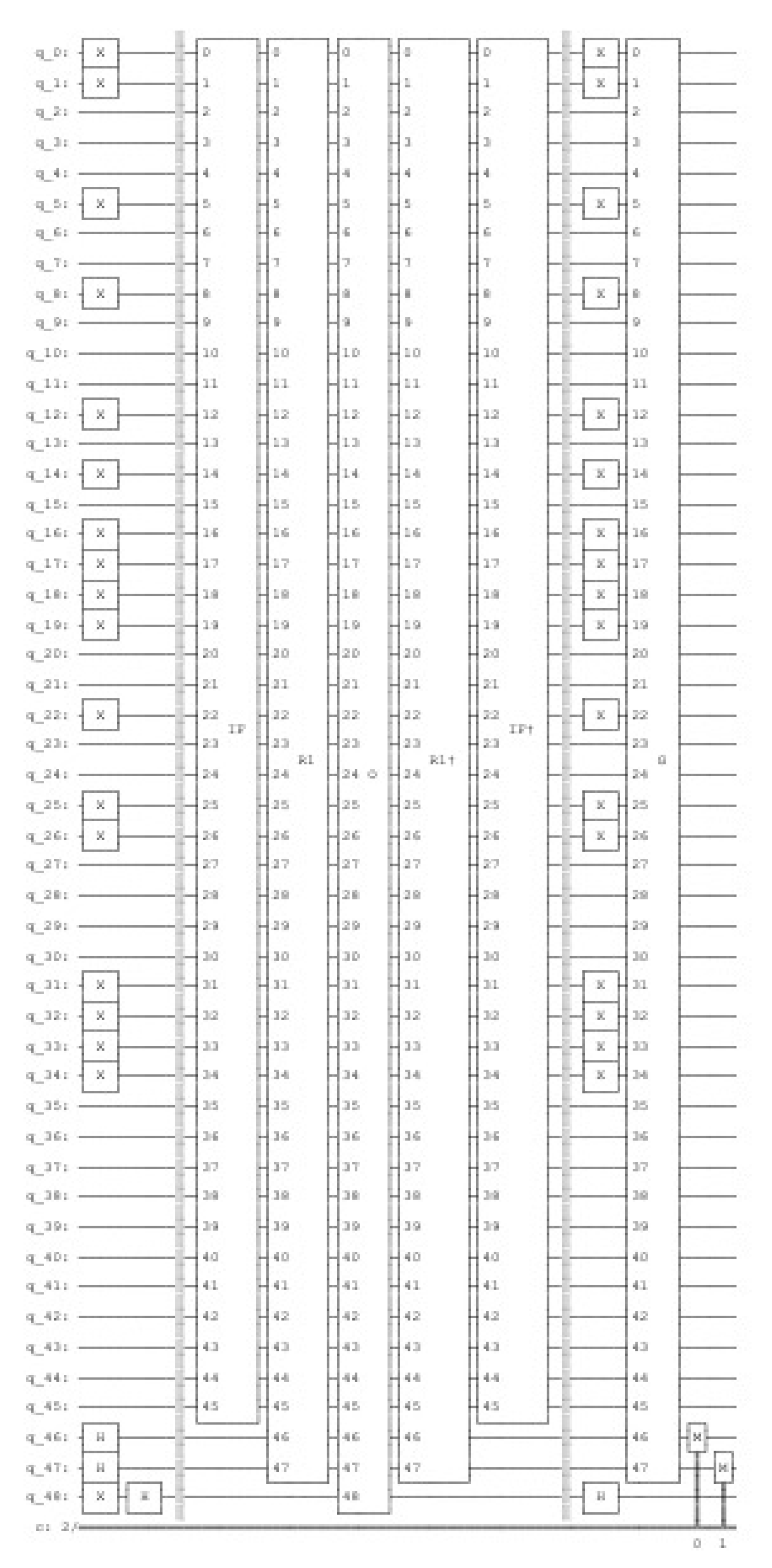
Figure 15.
The quantum circuit for the 9-puzzle task of the depth search 1. Simulating 36 qubits requires higher memory capacity, we cannot use the statevector simulator or a search depth of two due to memory constraints. The path descriptor has four possible states represented by two qubits and is measured after applying the function .

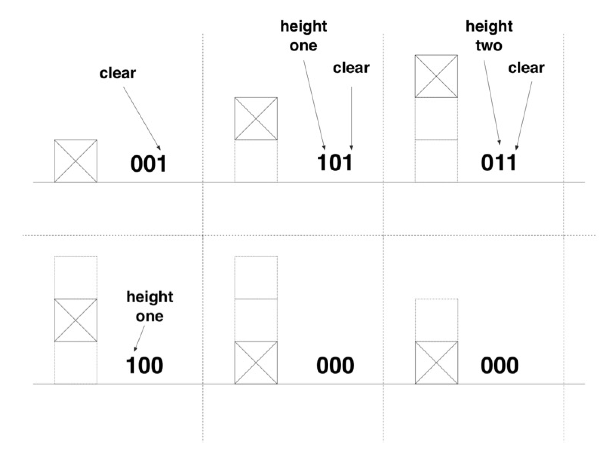
Figure 16.
Three qubits (bits) for each block represent its state. The first qubit equaling one indicates that the block is on top of one other block. The second qubit equaling one indicates that the block is on top of two other blocks. The third qubit equaling one indicates that the block is clear with nothing on top of it.

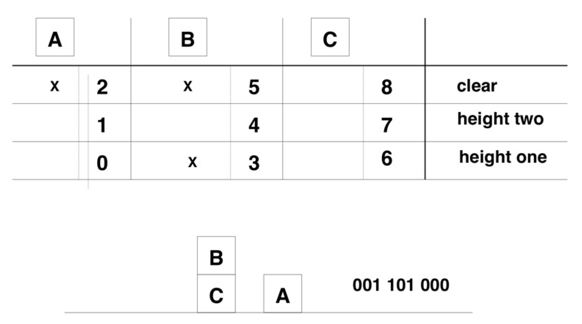
Figure 17.
Representing a state of A, B, C blocks by 9 qubits (bits). The class descriptor is fixed and the position descriptor (adjective) moves (is changed). Three qubits (bits) for each block represent its state. Their value changes indicating different states. On top, we see the three A, B, C blocks and the 9 positions of the qubits by the index from 0 to 9, x indicates that the qubit is equal to one. Below, we represent the corresponding state and the corresponding binary string.

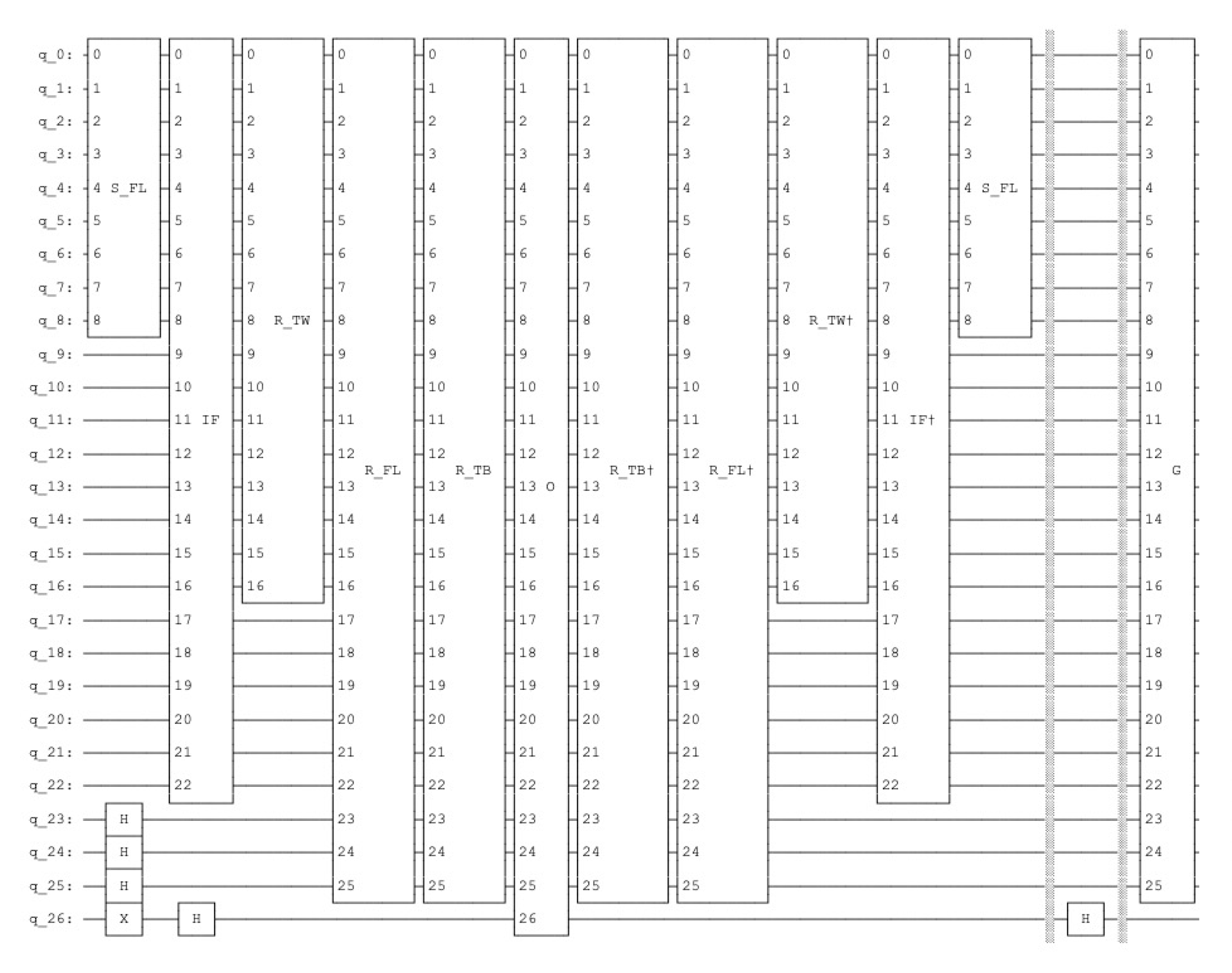
Figure 18.
The quantum circuit for the ABC blocks task of the depth search 1. Since we are using the statevector simulator, we do not need any measurement since the simulator determines the exact probabilities of each qubit. The circuit’s depth in the number of quantum gates is 13. The path descriptor has eight possible states represented by three qubits.

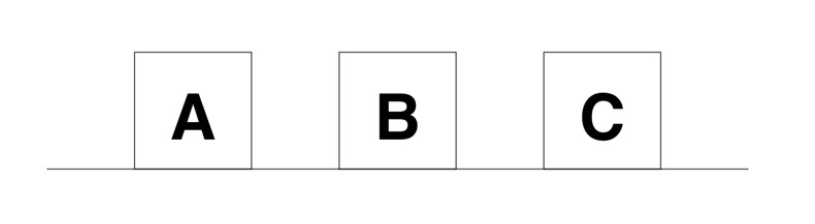
Figure 19.
The class all blocks on the floor has one combination.

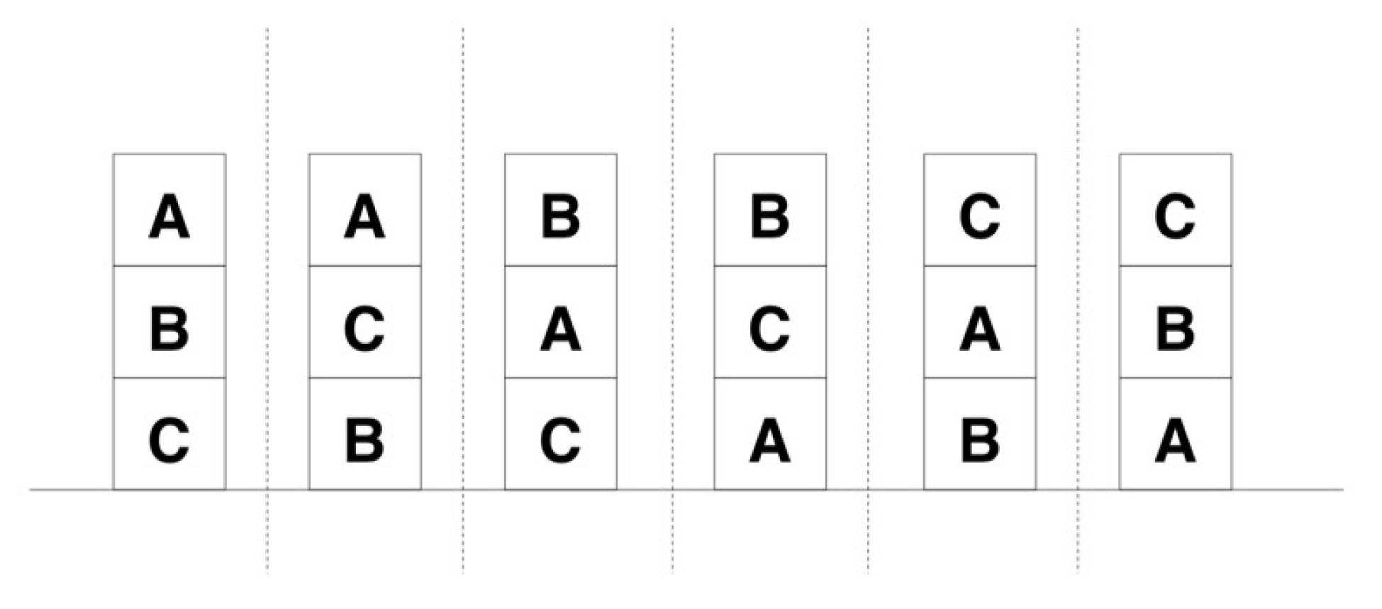
Figure 20.
The class tower appears in six different combinations.

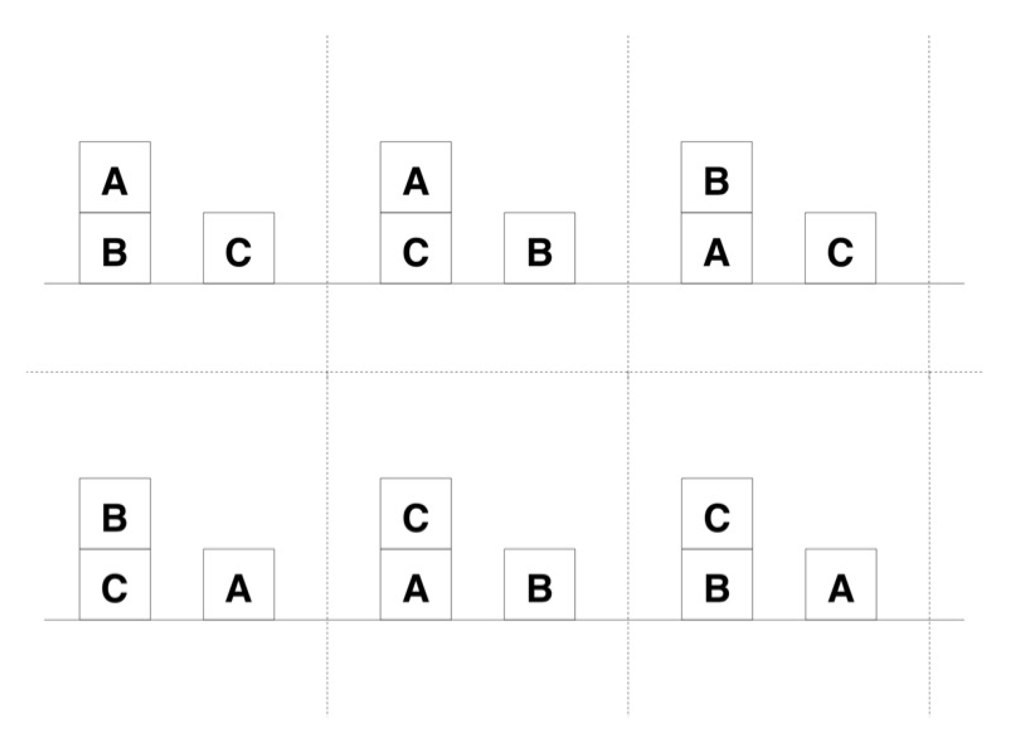
Figure 21.
The class small tower and a block on the table appears in six different combinations.

Figure 22.
One marked state results in a solution after one iteration indicated for the initial state all blocks on the floor and the goal states and B. The solution is described by the path descriptor by the qubits 23, 24 and 25 with the binary value 101, the fifth branch. There are 8 branches described by 8 possible transitions .

Figure 23.
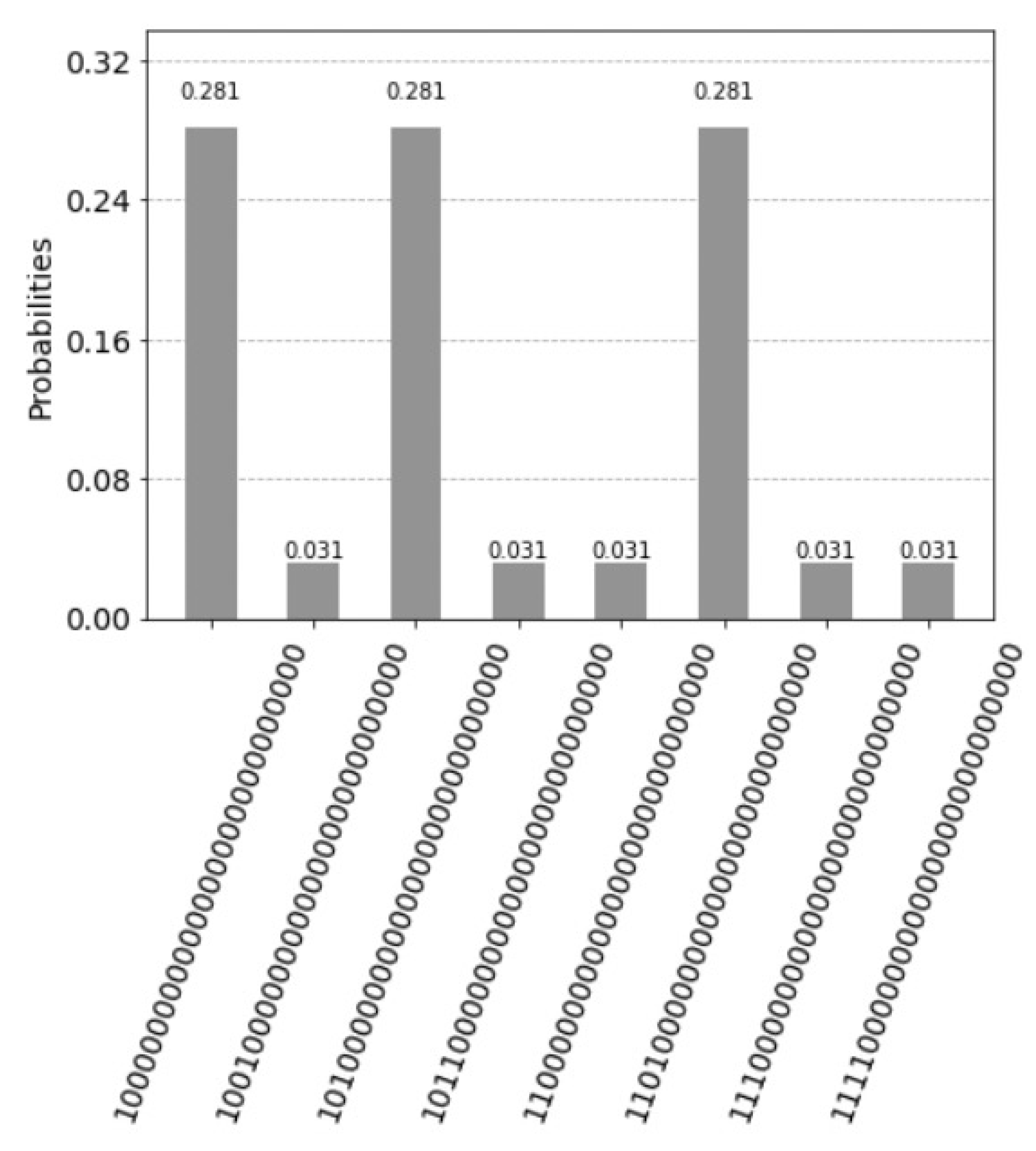
Three marked states results in a solution after one iteration indicated for the initial state and A and the goal states and B by the statevector simulator.
Figure 23.
Three marked states results in a solution after one iteration indicated for the initial state and A and the goal states and B by the statevector simulator.

Publisher’s Note: MDPI stays neutral with regard to jurisdictional claims in published maps and institutional affiliations. |
© 2022 by the author. Licensee MDPI, Basel, Switzerland. This article is an open access article distributed under the terms and conditions of the Creative Commons Attribution (CC BY) license (https://creativecommons.org/licenses/by/4.0/).
Share and Cite
MDPI and ACS Style
Wichert, A. Quantum Tree Search with Qiskit. Mathematics 2022, 10, 3103. https://doi.org/10.3390/math10173103
AMA Style
Wichert A. Quantum Tree Search with Qiskit. Mathematics. 2022; 10(17):3103. https://doi.org/10.3390/math10173103
Chicago/Turabian StyleWichert, Andreas. 2022. "Quantum Tree Search with Qiskit" Mathematics 10, no. 17: 3103. https://doi.org/10.3390/math10173103
Note that from the first issue of 2016, this journal uses article numbers instead of page numbers. See further details here.