Soliton Solutions of Klein–Fock–Gordon Equation Using Sardar Subequation Method

Abstract

The Klein–Fock–Gordon equation (KFGE), defined as the equation of relativistic wave related to NLEEs, has numerous implications for energy particle physics and is useful as a model for several types of matter, with deviation in the basic stuffs of particles and in crystals. In this work, the Sardar subequation method (SSM) is used for finding the solution of this KFGE. The advantage of SSM is that it provides many different kinds of solitons, such as dark, bright, singular, periodic singular, combined dark–singular and combined dark–bright solitons. The results show that the SSM is very reliable, simple and can be functionalized to other nonlinear equations. It is verified that all the attained solutions are stable by modulation instability process. To enhance the physical description of solutions, some 3D, contour and 2D graphs are plotted by taking precise values of parameters using Maple 18.

1. Introduction

In past years, nonlinear problems have been observed by physicists, engineers, mathematicians and numerous further researchers. Nowadays, the NLEEs have become the topic of analysis in branches of nonlinear fields, such as plasma physics, mathematical fluid dynamics, propagation of shallow water wave, protein chemistry, applied mathematics, physics, geochemistry, chemically reactive materials, chemical kinematics, meteorology, etc. The work on soliton wave solutions of NLEEs is increasingly receiving much attention [1,2,3,4,5,6,7,8,9,10]. Our suggested model, 3rd-order KFGE, is an imperative part of NLEEs, applicable in various kinds of matter, having many implications in quantum mechanics and energy particle physics. It explains quantum amplitude for exploring the particle in various fields while the particle has backward and forward motion [11]. Sometimes the equation of relativistic wave associated with the Schrodinger equation is also called KFGE. There are many papers in which different types of KFGE are explored. In 2009, Rayan Samsun studied the model of KFGE with power law nonlinearity by using perturbation theory [12]. Biswas et al. [13] explained the theory of quadratic KFGE with the help of perturbation terms. Khalique et al. [14] used the lie symmetric method to study the KFGE and obtained non-trivial solutions. Biswas et al. [15] implemented the bifurcation analysis on KFGE that yielded a new set of solutions. Shahen et al. [16] explained the interaction between the Phi-4 equation in term of conformable fractional derivative, and obtained kink, periodic and lump solutions. Biswas and Chawdhury [17] studied the numerical and soliton solutions of the Phi-4 equation, written as

$$\begin{array}{c}\hfill {\mu }_{tt}+k^2{\mu }_{xx}=a\mu +b{\mu }^3.\end{array}$$

If we replace $k^2=c$, $a=-\gamma$ and $b=-\delta$, then KFGE is reduced into 3rd-order KFGE [16,17,18,19], written as

$$\begin{array}{c}\hfill {\mu }_{tt}+c{\mu }_{xx}+\gamma \mu +\delta {\mu }^3=0.\end{array}$$

(1)

where $\mu (x,t)$ is the wave profile of the particle, and c, $\gamma$, and $\delta$ are real constants. This model equation explains the dispersion of dislocations in crystals, the distribution of splay wave, the theory of elementary particles, the dispersion of magnetic flux along a Josephson line, etc. [19]. Nowadays, many researchers are investigating exact solutions for NLEEs by using different methods. Many powerful techniques have been offered, such as the exp-function expansion scheme [20], the Hirotas bilinear transformation method [21], the $exp(-\psi (\xi \left)\right)$-expansion method [22,23,24], the Lie symmetry technique [25,26,27,28], the extended tanh-function technique [29,30], the complex hyperbolic function technique [31], the modified simple equation scheme [32,33], the $(G^{\prime }/G)$-expansion scheme [34,35,36], the Bernoullis sub-ODE scheme [37], Jacobi elliptic technique [38], the enhanced $(G/G)$-expansion approach [39], He’s polynomial methods [40,41], the homogeneous balance scheme [42,43], the variational iteration method, the Riccati equation expansion method [44], and so on [45,46,47]. The purpose of this article is to efficiently employ SSM [48,49,50,51,52] for finding exact solutions of KFGE. In this study, using SSM, novel solutions in the form of hyperbolic and trigonometric functions are obtained that build bright, singular, dark, periodic singular, combined dark–singular and combined dark–bright solitons [53,54].

The paper is arranged as follows: In Section 2, the description of the method is explained. In Section 3, we construct the solution of KFGE. In Section 4, the stability analysis of the obtained solution is given. In Section 5, the physical explanation of the graphs is discussed. Section 6 gives the comparison. Conclusions are given in the last section.

2. Description of the Method

In this part, a description of SSM [48] is given. In the first step, we suppose NLPDE

$$\begin{array}{c}\hfill G(\mu ,{\mu }_t,{\mu }_x,{\mu }_{tt},{\mu }_{xx},...)=0,\end{array}$$

(2)

Consider the transformation

$$\begin{array}{c}\hfill \mu (x,t)=Z\left(\chi \right),\chi =nx-dt.\end{array}$$

(3)

By inserting (3) into (2), we obtain

$$\begin{array}{c}\hfill R(Z,Z^{\prime },Z^{″},Z^{‴},...)=0,\end{array}$$

(4)

where $Z=Z(\chi$), $Z^{\prime }=\frac{dZ}{d\chi }$, $Z^{″}=\frac{d^{2}Z}{d{\chi }^2}.$

Suppose (4) has a solution

$$\begin{array}{c}\hfill Z\left(\chi \right)=\sum _{i=0}^s{\omega }_i{\psi }^i\left(\chi \right),{\omega }_s\ne 0.\end{array}$$

(5)

where ${\omega }_i$, (i = 0, 1, 2, ..., s) are coefficients to be found later, $\psi \left(\chi \right)$ satisfies the ODE in the form

$$\begin{array}{c}\hfill {\left({\psi }^{\prime }\left(\chi \right)\right)}^2=\sigma +g{\psi }^2\left(\chi \right)+{\psi }^4\left(\chi \right),\end{array}$$

(6)

where $\sigma$ and g are fixed real constants, and the solutions of (6) are as follows.

Case 1: If $\sigma$ = 0 and $g>0$ then

$${\psi }_1^{\pm }\left(\chi \right)=\pm \sqrt{-pqg}sec{h}_{pq}\left(\sqrt{g}\chi \right),$$

$${\psi }_2^{\pm }\left(\chi \right)=\pm \sqrt{pqg}csc{h}_{pq}\left(\sqrt{g}\chi \right),$$

where

$$sec{h}_{pq}\left(\chi \right)=\frac{2}{p{e}^{\chi }+q{e}^{-\chi }},csc{h}_{pq}\left(\chi \right)=\frac{2}{p{e}^{\chi }-q{e}^{-\chi }}.$$

Case 2: If $\sigma$ = 0 and $g<0$ then

$${\psi }_3^{\pm }\left(\chi \right)=\pm \sqrt{-pqg}se{c}_{pq}\left(\sqrt{-g}\chi \right),$$

$${\psi }_4^{\pm }\left(\chi \right)=\pm \sqrt{-pqg}cs{c}_{pq}\left(\sqrt{-g}\chi \right),$$

where

$$se{c}_{pq}\left(\chi \right)=\frac{2}{p{e}^{\iota \chi }+q{e}^{-\iota \chi },}cs{c}_{pq}\left(\chi \right)=\frac{2\iota }{p{e}^{\iota \chi }-q{e}^{-\iota \chi }}.$$

Case 3: If $g<0$ and $\sigma =\frac{g^2}{4}$ then

$${\psi }_5^{\pm }\left(\chi \right)=\pm \sqrt{\frac{-g}{2}}tan{h}_{pq}\left(\sqrt{\frac{-g}{2}}\chi \right),$$

$${\psi }_6^{\pm }\left(\chi \right)=\pm \sqrt{\frac{-g}{2}}cot{h}_{pq}\left(\sqrt{\frac{-g}{2}}\chi \right),$$

$${\psi }_7^{\pm }\left(\chi \right)=\pm \sqrt{\frac{-g}{2}}(tan{h}_{pq}\left(\sqrt{-2g}\chi \right)\pm \iota \sqrt{pq}sec{h}_{pq}\left(\sqrt{-2g}\chi \right)),$$

$${\psi }_8^{\pm }\left(\chi \right)=\pm \sqrt{\frac{-g}{2}}(cot{h}_{pq}\left(\sqrt{-2g}\chi \right)\pm \sqrt{pq}csc{h}_{pq}\left(\sqrt{-2g}\chi \right)),$$

$${\psi }_9^{\pm }\left(\chi \right)=\pm \sqrt{\frac{-g}{2}}(tan{h}_{pq}\left(\sqrt{\frac{-g}{2}}\chi \right)+cot{h}_{pq}\left(\sqrt{\frac{-g}{2}}\chi \right)),$$

where

$$tan{h}_{pq}\left(\chi \right)=\frac{p{e}^{\chi }-q{e}^{-\chi }}{p{e}^{\chi }+q{e}^{-\chi }},cot{h}_{pq}\left(\chi \right)=\frac{p{e}^{\chi }+q{e}^{-\chi }}{p{e}^{\chi }-q{e}^{-\chi }}.$$

Case 4: If $g>0$ and $\rho =\frac{g^2}{4}$ then

$${\psi }_{10}^{\pm }\left(\chi \right)=\pm \sqrt{\frac{g}{2}}ta{n}_{pq}\left(\sqrt{\frac{g}{2}}\chi \right),$$

$${\psi }_{11}^{\pm }\left(\chi \right)=\pm \sqrt{\frac{g}{2}}co{t}_{pq}\left(\sqrt{\frac{g}{2}}\chi \right),$$

$${\psi }_{12}^{\pm }\left(\chi \right)=\pm \sqrt{\frac{g}{2}}(ta{n}_{pq}\left(\sqrt{2g}\chi \right)\pm \sqrt{pq}se{c}_{pq}\left(\sqrt{2g}\chi \right)),$$

$${\psi }_{13}^{\pm }\left(\chi \right)=\pm \sqrt{\frac{g}{2}}(co{t}_{pq}\left(\sqrt{2g}\chi \right)\pm \sqrt{pq}cs{c}_{pq}\left(\sqrt{2g}\chi \right)),$$

$${\psi }_{14}^{\pm }\left(\chi \right)=\pm \sqrt{\frac{g}{2}}(ta{n}_{pq}\left(\sqrt{\frac{g}{2}}\chi \right)+co{t}_{pq}\left(\sqrt{\frac{g}{2}}\chi \right)),$$

where

$$ta{n}_{pq}\left(\chi \right)=-\iota \frac{p{e}^{\chi }-q{e}^{-\chi }}{p{e}^{\chi }+q{e}^{-\chi }},co{t}_{pq}\left(\chi \right)=\iota \frac{p{e}^{\chi }+q{e}^{-\chi }}{p{e}^{\chi }-q{e}^{-\chi }}.$$

First, we find s in (5) by the balancing rule. After finding s, put (5) and (6) into (4), and we obtain the equation in powers of $\psi \left(\chi \right)$. After obtaining a non-zero solution, insert all coefficients of $\psi \left(\chi \right)$ equal to zero, and we obtain the system of algebraic equations. By solving this system, we find solutions. After inserting these solutions with solutions of (6), we can find values of (3).

3. Construction of Solutions of KFGE

In this section, we construct solutions of KFGE.

Let

$$\begin{array}{c}\hfill \mu (x,t)=Z\left(\chi \right),\chi =nx-dt.\end{array}$$

(7)

By inserting (7) into (1), we obtain

$$\begin{array}{c}\hfill Z^{″}(d^2+c{n}^2)+\delta Z^3+\gamma Z=0,\end{array}$$

(8)

By balancing the nonlinear term of the highest order $Z^3$ with higher-order derivative $Z^{″}$, we obtain s = 1 which turns (5) into

$$\begin{array}{c}\hfill Z\left(\chi \right)={\omega }_0+{\omega }_1\psi \left(\chi \right),\end{array}$$

(9)

Now by inserting (9) and (6) into Equation (8), we obtain algebraic equations in terms of powers of $\psi \left(\chi \right)$. By putting coefficients of all $\psi \left(\chi \right)$ equal to zero, the following system is

$$\begin{array}{ccc}& & \gamma {\omega }_0+\delta {\omega }_0^3=0,\hfill \\ & & g{d}^2{\omega }_1+gc{n}^2{\omega }_1+\gamma {\omega }_1+3\delta {\omega }_0^2{\omega }_1=0,\hfill \\ & & 3\delta {\omega }_0{\omega }_1^2=0,\hfill \\ & & 2d^2{\omega }_1+\delta {\omega }_1^3+2c{n}^2{\omega }_1=0.\hfill \end{array}$$

Now by solving this system, we obtain the following values of constants:

$$\begin{array}{ccc}\hfill & & {\omega }_0=0,\hfill \\ & & {\omega }_1=\pm \frac{\sqrt{2}\sqrt{-d^2-c{n}^2}}{\sqrt{\gamma }},\hfill \\ & & g=-\frac{\gamma }{d^2+c{n}^2}.\hfill \end{array}$$

(10)

Now by inserting these constants and solutions of (6) in (9), we obtain the following solutions.

Case 1: If $g=-\frac{\gamma }{d^2+c{n}^2}>0$ and $\sigma =0$

$$\begin{array}{ccc}& & Z_1=\pm \frac{\sqrt{2}\sqrt{-c{n}^2-d^2}}{\sqrt{\delta }}\left(\left.\pm \sqrt{\frac{\gamma pq}{c{n}^2+d^2}}\right){\mathit{sec}h}_{\mathit{pq}}\left(\sqrt{\frac{-\gamma }{c{n}^2+d^2}}\chi \right)\right.,\hfill \\ & & Z_2=\pm \frac{\sqrt{2}\sqrt{-c{n}^2-d^2}}{\sqrt{\delta }}\left(\left.\pm \sqrt{\frac{\gamma pq}{c{n}^2+d^2}}\right){\mathit{csc}h}_{\mathit{pq}}\left(\sqrt{\frac{-\gamma }{c{n}^2+d^2}}\chi \right)\right..\hfill \end{array}$$

Case 2: If $g=-\frac{\gamma }{d^2+c{n}^2}<0$ and $\sigma =0$

$$\begin{array}{ccc}& & Z_3=\pm \frac{\sqrt{2}\sqrt{-c{n}^2-d^2}}{\sqrt{\delta }}\left(\left.\pm \sqrt{\frac{\gamma pq}{c{n}^2+d^2}}\right){\mathit{sec}}_{\mathit{pq}}\left(\sqrt{\frac{\gamma }{c{n}^2+d^2}}\chi \right)\right.,\hfill \\ & & Z_4=\pm \frac{\sqrt{2}\sqrt{-c{n}^2-d^2}}{\sqrt{\delta }}\left(\left.\pm \sqrt{\frac{\gamma pq}{c{n}^2+d^2}}\right){\mathit{csc}}_{\mathit{pq}}\left(\sqrt{\frac{\gamma }{c{n}^2+d^2}}\chi \right)\right..\hfill \end{array}$$

Case 3: If $g=-\frac{\gamma }{d^2+c{n}^2}<0$ and $\sigma =\frac{g^2}{4}$

$$\begin{array}{ccc}& & Z_5=\pm \frac{\sqrt{2}\sqrt{-c{n}^2-d^2}}{\sqrt{\delta }}\left(\left.\sqrt{\frac{\gamma }{2(c{n}^2+d^2)}}\right){\mathit{tan}h}_{\mathit{pq}}\left(\sqrt{\frac{\gamma }{2(c{n}^2+d^2)}}\chi \right)\right.,\hfill \\ & & Z_6=\pm \frac{\sqrt{2}\sqrt{-c{n}^2-d^2}}{\sqrt{\delta }}\left(\left.\sqrt{\frac{\gamma }{2(c{n}^2+d^2)}}\right){\mathit{cot}h}_{\mathit{pq}}\left(\sqrt{\frac{\gamma }{2(c{n}^2+d^2)}}\chi \right)\right.,\hfill \\ & & Z_7=\pm \frac{\sqrt{2}\sqrt{-c{n}^2-d^2}}{\sqrt{\delta }}\left(\sqrt{\frac{\gamma }{2(c{n}^2+d^2)}}\left({\mathit{tan}h}_{\mathit{pq}}\left(\sqrt{\frac{2\gamma }{c{n}^2+d^2}}\chi \right)\pm \sqrt{-pq}{\mathit{sec}h}_{\mathit{pq}}\left(\sqrt{\frac{2\gamma }{c{n}^2+d^2}}\chi \right)\right)\right),\hfill \\ & & Z_8=\pm \frac{\sqrt{2}\sqrt{-c{n}^2-d^2}}{\sqrt{\delta }}\left(\sqrt{\frac{\gamma }{2(c{n}^2+d^2)}}\left({\mathit{cot}h}_{\mathit{pq}}\left(\sqrt{\frac{2\gamma }{c{n}^2+d^2}}\chi \right)\pm \sqrt{-pq}{\mathit{csc}h}_{\mathit{pq}}\left(\sqrt{\frac{2\gamma }{c{n}^2+d^2}}\chi \right)\right)\right),\hfill \\ & & Z_9=\pm \frac{\sqrt{2}\sqrt{-c{n}^2-d^2}}{\sqrt{\delta }}\left(\frac{\sqrt{\frac{\gamma }{2(c{n}^2+d^2)}}}{2}\left({\mathit{cot}h}_{\mathit{pq}}\left(\frac{\sqrt{\frac{\gamma }{2(c{n}^2+d^2)}}}{2}\chi \right)+{\mathit{tan}h}_{\mathit{pq}}\left(\frac{\sqrt{\frac{\gamma }{2(c{n}^2+d^2)}}}{2}\chi \right)\right)\right).\hfill \end{array}$$

Case 4: If $g=-\frac{\gamma }{d^2+c{n}^2}>0$ and $\sigma =\frac{g^2}{4}$

$$\begin{array}{ccc}& & Z_{10}=\pm \frac{\sqrt{2}\sqrt{-c{n}^2-d^2}}{\sqrt{\delta }}\left(\left.\sqrt{\frac{-\gamma }{2(c{n}^2+d^2)}}\right){\mathit{tan}}_{\mathit{pq}}\left(\sqrt{\frac{-\gamma }{2(c{n}^2+d^2)}}\chi \right)\right.,\hfill \\ & & Z_{11}=\pm \frac{\sqrt{2}\sqrt{-c{n}^2-d^2}}{\sqrt{\delta }}\left(\left.\sqrt{\frac{-\gamma }{2(c{n}^2+d^2)}}\right){\mathit{cot}}_{\mathit{pq}}\left(\sqrt{\frac{-\gamma }{2(c{n}^2+d^2)}}\chi \right)\right.,\hfill \\ & & Z_{12}=\pm \frac{\sqrt{2}\sqrt{-c{n}^2-d^2}}{\sqrt{\delta }}\left(\sqrt{\frac{-\gamma }{2(c{n}^2+d^2)}}\left({\mathit{tan}}_{\mathit{pq}}\left(\sqrt{\frac{-2\gamma }{c{n}^2+d^2}}\chi \right)\pm \sqrt{-pq}{\mathit{sec}}_{\mathit{pq}}\left(\sqrt{\frac{-2\gamma }{c{n}^2+d^2}}\chi \right)\right)\right),\hfill \\ & & Z_{13}=\pm \frac{\sqrt{2}\sqrt{-c{n}^2-d^2}}{\sqrt{\delta }}\left(\sqrt{\frac{-\gamma }{2(c{n}^2+d^2)}}\left({\mathit{cot}}_{\mathit{pq}}\left(\sqrt{\frac{-2\gamma }{c{n}^2+d^2}}\chi \right)\pm \sqrt{-pq}{\mathit{csc}}_{\mathit{pq}}\left(\sqrt{\frac{-2\gamma }{c{n}^2+d^2}}\chi \right)\right)\right),\hfill \\ & & Z_{14}=\pm \frac{\sqrt{2}\sqrt{-c{n}^2-d^2}}{\sqrt{\delta }}\left(\frac{\sqrt{\frac{-\gamma }{2(c{n}^2+d^2)}}}{2}\left({\mathit{cot}}_{\mathit{pq}}\left(\frac{\sqrt{\frac{-\gamma }{2(c{n}^2+d^2)}}}{2}\chi \right)+{\mathit{tan}}_{\mathit{pq}}\left(\frac{\sqrt{\frac{-\gamma }{2(c{n}^2+d^2)}}}{2}\chi \right)\right)\right).\hfill \end{array}$$

4. Stability Analysis

Sometimes, many nonlinear models manifest instability, which guides us to explore the modulation of the steady-state position as a result of obstruction between the nonlinear and dispersive effects, which gives the linear stability analysis [55].

To establish the stability analysis of KFGE (1) by utilizing the linear stability analysis [55,56], consider the following solution of KFGE as

$$\mu (x,t)=A\varphi (x,t)+L_0,$$

(11)

where $L_0$ is the constant which shows the steady-state solution of (1). Substituting (11) into (1), and linearizing the equation in A, we obtain

$$A{\varphi }_{tt}+cA{\varphi }_{xx}+(\gamma A+3\delta L_0^{2}A)\varphi =0.$$

(12)

Consider the solution of (12) as

$$\varphi (x,t)=e^{\iota (nx-\omega t)}.$$

(13)

where n and $\omega$ are the normalized frequency and wave number of $\varphi (x,t)$. Substituting (13) into (12), we attain the relation as

$$\omega =\sqrt{-c{n}^2+\gamma +3\delta L_0^2}.$$

(14)

When $-c{n}^2+\gamma +3\delta L_0^2>0$, i.e., $\omega$ is real, the steady state is stable along the small perturbation. It becomes unstable when $-c{n}^2+\gamma +3\delta L_0^2<0$, i.e., $\omega$ is imaginary as the perturbation develops exponentially. One can simply observe modulation instability (MI) when $-c{n}^2+\gamma +3\delta L_0^2<0$.

5. Results and Discussion

In this part, the graphical representation and physical explanation of some solutions of KFGE equation are discussed. With the aid of Maple 18, some graphs of derived solutions are drawn that have particular importance in wave soliton theory. Different types of soliton solutions based on district values of parameters are given in Figure 1, Figure 2, Figure 3, Figure 4 and Figure 5.

5.1. Physical and Geometrical Interpretation

This subsection addresses the physical and geometrical interpretations of solutions of KFGE by using the SSM. The advantage of the used method is that it provides abundant and general soliton solutions under different parameters. We illustrate 3D, contour and 2D plots with the help of Maple 18. A 3D plot is used to show the visual importance of wave dispersion; the contour plots allow to visualize three-dimensional data in a two-dimensional plot; and the 2D plot is drawn to check the phase component and amplitude of the solutions clearly.

The obtained solutions $Z_1(x,t)$, $Z_2(x,t)$, $Z_5(x,t)$, $Z_6(x,t)$, $Z_7(x,t)$, $Z_8(x,t)$, $Z_9(x,t)$ are solutions of hyperbolic functions, while the remaining solutions $Z_3(x,t)$, $Z_4(x,t)$, $Z_{10}(x,t)$, $Z_{11}(x,t)$, $Z_{12}(x,t)$, $Z_{13}(x,t)$, $Z_{14}(x,t)$ are obtained from trigonometric functions. $Z_2(x,t)$, $Z_6(x,t)$, and $Z_8(x,t)$ represent properties of singular solitons, so we illustrated only $Z_6(x,t)$. Similarly, $Z_3(x,t)$, $Z_4(x,t)$, $Z_{10}(x,t)$, $Z_{11}(x,t)$, $Z_{12}(x,t)$, $Z_{13}(x,t)$, and $Z_{14}(x,t)$ have the properties of periodic solitons, so we considered only $Z_4(x,t)$.

The 3D plot and contour plot of soliton solutions $Z_1(x,t)$ are drawn in Figure 1a,b, respectively which elaborates the bright solitons for the values of $\gamma =-0.5$, d = 1, c = 0.5, n = 0.98, p = 0.98, q = 0.95, $\delta =1$ with the interval $-10\le x\le 10$, $-10\le t\le 10$, while Figure 1c represents the 2D view of $Z_1(x,t)$ when $-10\le x\le 10$ and $t=0$ are taken. It can be observed that the amplitude of soliton $Z_1(x,t)$ increases when the value of d decreases, and the phase component of the soliton changes.

For the values of $\gamma =0.5$, d = 1, c = 0.5, n = 0.98, p = 0.98, q = 0.95, $\delta =1$ with the interval $-10\le x\le 10$, $-10\le t\le 10$, the graph of $Z_4(x,t)$ describes the shape of the periodic soliton as shown in Figure 2a, Figure 2b represents the contour graph of $Z_4(x,t)$, and the 2D plot is drawn in Figure 2c. By changing the values of the parameters, variations in the phase component and amplitude are observed.

The wave profile of $Z_5(x,t)$ elaborates the shape of dark solitons when waves transmit along the x and t axes as shown in Figure 3a for the values of $\gamma =0.5$, d = 1, c = 0.5, n = 0.98, p = 0.98, q = 0.95, $\delta =1$ with the interval $-10\le x\le 10$, $-10\le t\le 10$. Figure 3b demonstrates the contour graph, while in Figure 3c, the 2D plot is drawn at $t=0$. It can be noticed the amplitude increases and the phase component also varies when the value of d decreases.

To describe $Z_6(x,t)$, we illustrate a 3D plot which shows the singular soliton shape by selecting the values of $\gamma =0.5$, d = 1, c = 0.5, n = 0.98, p = 0.98, q = 0.95, $\delta =1$$-10\le x\le 10$, $-10\le t\le 10$ as shown in Figure 4a. Figure 4b shows the contour plot of solution $Z_6(x,t)$. The amplitude increases, and the phase component of $Z_6(x,t)$ shows variation by changing the value of d, which can be seen clearly in the 2D representation of $Z_6(x,t)$.

For the solution of $Z_7(x,t)$, Figure 5a elaborates the 3D wave profile, which represents combined bright–dark soliton by considering the values $\gamma =-0.5$, d = 1, c = 0.5, n = 0.98, p = 0.98, q = 0.95, $\delta =1$$-10\le x\le 10$, $-10\le t\le 10$. Figure 5b,c represent the contour and 2D graph of $Z_7(x,t)$ respectively. The changing in phase and amplitude component can be observed as the value of d decreases.

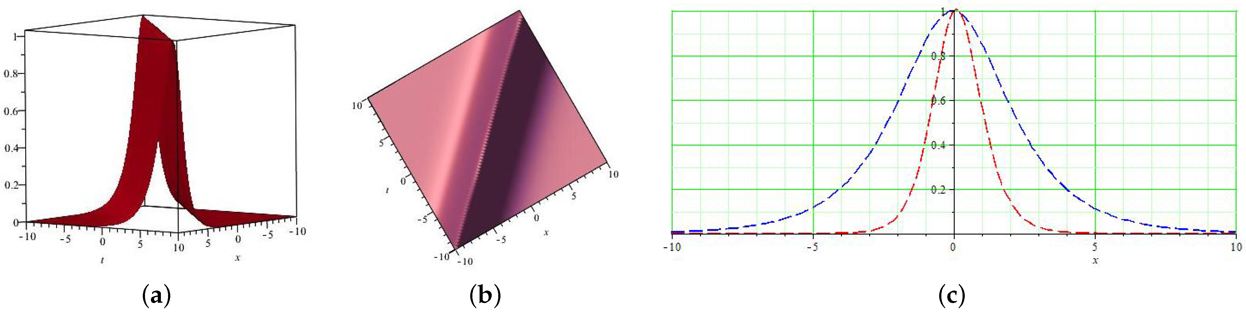
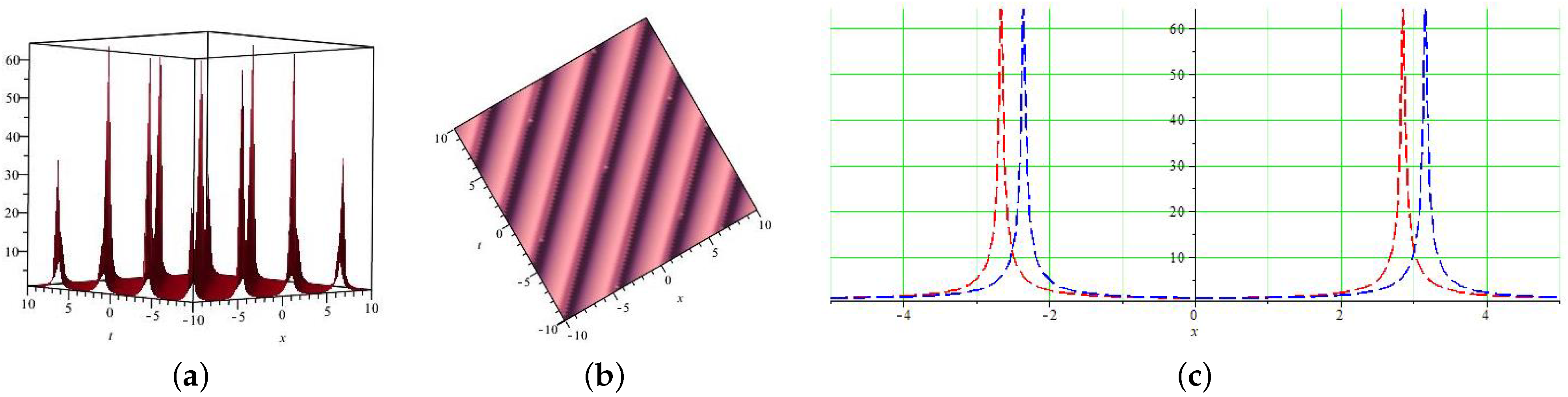
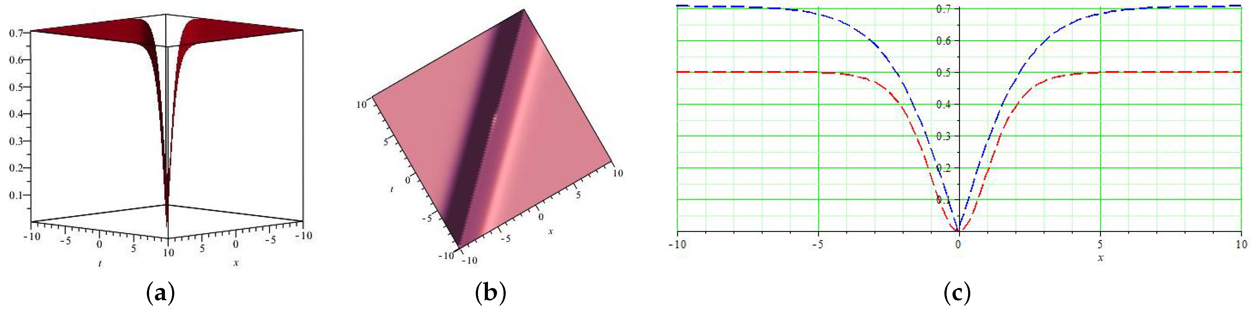
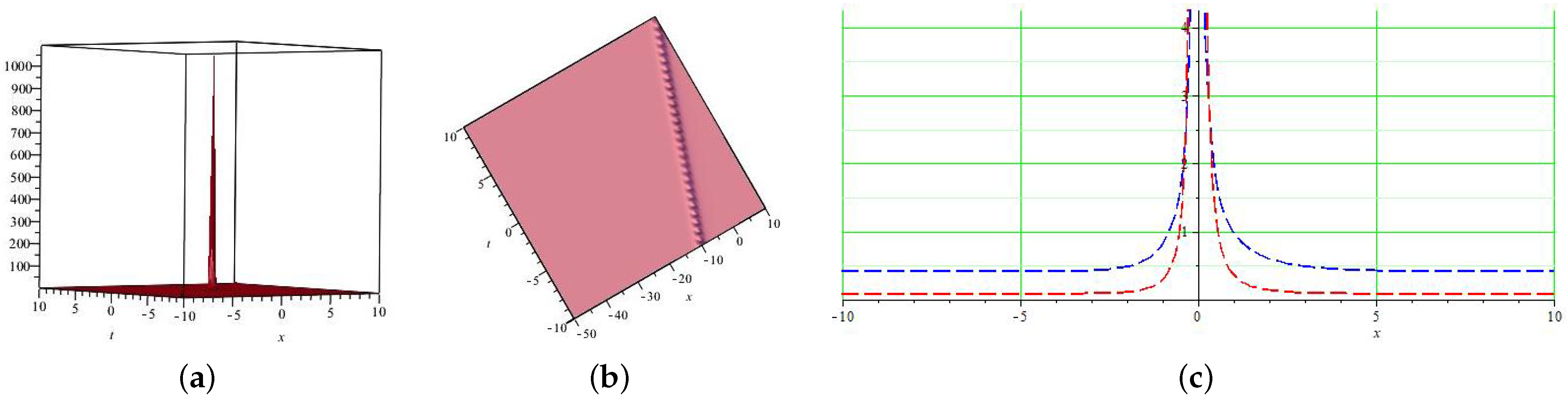
5.2. Graphical Representation

This subsection displays the graphical illustrations of some solutions of KFGE. For the plotting of graphs, we used the Maple 18 software.

6. Comparison

The Klein–Fock–Gordon equation (KFGE) is explored many times by applying other schemes. In this section, we compare our results with the results of some earlier work obtained by other schemes, such as the modified F-expansion method, extended simple equation method and modified $\left(\frac{G^{\prime }}{G}\right)$-$expansion$ method [18,57].

• The extended simple equation method provides dark soliton, singular soliton and periodic singular solutions; the modified F-expansion method elaborates singular soliton and combined dark–singular soliton solutions; and the modified $\left(\frac{G^{\prime }}{G}\right)$-$expansion$ method extracts dark, singular, combined dark–singular and periodic singular soliton solutions for KFGE.
• In this paper, we obtain 14 novel solutions of KFGE based on trigonometric and hyperbolic functions. Our present method (Sardar subequation method) establishes six different types of solutions, i.e., bright soliton, dark soliton, singular soliton, periodic singular soliton, combined dark–bright soliton and combined dark–singular soliton solutions.

7. Conclusions

In the current work, we applied the SSM to find the solutions for KFGE. The results obtained are of the form of hyperbolic and trigonometric functions, which provide bright, singular, dark, periodic singular, combined dark–bright, and combined dark–singular soliton solutions. Some of these solutions are graphically displayed by the 3D, 2D and contour graphs for better understanding. By comparing the SSM with existing methods, we can assert that this method provides many different types of solutions, as compared to others [18,57]. The stability of the solutions is also discussed by the modulation instability process. Moreover, it is noted that this method is convincing, reliable and can easily be applied to other NLEEs. Physicists can apply these results for further applications.

References

1. Seadawy, A.R. Stability analysis for Zakharov–Kuznetsov equation of weakly nonlinear ion-acoustic waves in a plasma. Comput. Math. Appl. 2014, 67, 172–180. [Google Scholar] [CrossRef]
2. Solitons, M.A.P.C. Nonlinear Evolution Equations and Inverse SCattering; Cambridge University Press: Cambridge, UK, 1991; Volume 3, pp. 2301–2305. [Google Scholar]
3. Rehman, H.U.; Awan, A.U.; Abro, K.A.; El Din, E.M.T.; Jafar, S.; Galal, A.M. A non-linear study of optical solitons for Kaup-Newell equation without four-wave mixing. J. King Saud-Univ. Sci. 2022, 34, 102056. [Google Scholar] [CrossRef]
4. Seadawy, A.R. Stability analysis for two-dimensional ion-acoustic waves in quantum plasmas. Phys. Plasmas 2014, 21, 052107. [Google Scholar] [CrossRef]
5. Tahir, M.; Awan, A.U.; Rehman, H.U. Dark and singular optical solitons to the Biswas-Arshed model with Kerr and power law nonlinearity. Optik 2019, 185, 777–783. [Google Scholar] [CrossRef]
6. Dong, S.H. Wave Equations in Higher Dimensions; Springer Science Business Media: Berlin/Heidelberg, Germany, 2011. [Google Scholar]
7. Justin, M.; David, V.; Shahen, N.H.M.; Sylvere, A.S.; Rezazadeh, H.; Inc, M.; Betchewe, G.; Doka, S.Y. Sundry optical solitons and modulational instability in Sasa-Satsuma model. Opt. Quantum Electron. 2022, 54, 81. [Google Scholar] [CrossRef]
8. Shahen, N.H.M.; Bashar, M.H.; Tahseen, T.; Hossain, S. Solitary and rogue wave solutions to the conformable time fractional modified kawahara equation in mathematical physics. Adv. Math. Phys. 2021, 2021, 6668092. [Google Scholar] [CrossRef]
9. An, T.; Shahen, N.H.M.; Ananna, S.N.; Hossain, M.F.; Muazu, T. Exact and explicit travelling-wave solutions to the family of new 3D fractional WBBM equations in mathematical physics. Results Phys. 2020, 19, 103517. [Google Scholar]
10. Qian, L.; Attia, R.A.; Qiu, Y.; Lu, D.; Khater, M.M. The shock peakon wave solutions of the general Degasperis Procesi equation. Int. J. Mod. Phys. B 2019, 33, 1950351. [Google Scholar] [CrossRef]
11. Kumar, D.; Singh, J.; Kumar, S. Numerical computation of Klein-Gordon equations arising in quantum field theory by using homotopy analysis transform method. Alex. Eng. J. 2014, 53, 469–474. [Google Scholar] [CrossRef]
12. Sassaman, R.; Biswas, A. Soliton perturbation theory for phi-four model and nonlinear Klein-Gordon equations. Commun. Nonlinear Sci. Numer. Simul. 2009, 14, 3239–3249. [Google Scholar] [CrossRef]
13. Biswas, A.; Zony, C.; Zerrad, E. Soliton perturbation theory for the quadratic nonlinear Klein-Gordon equation. Appl. Math. Comput. 2008, 203, 153–156. [Google Scholar] [CrossRef]
14. Khalique, C.M.; Biswas, A. Analysis of non-linear Klein-Gordon equations using Lie symmetry. Appl. Math. Lett. 2010, 23, 1397–1400. [Google Scholar] [CrossRef]
15. Biswas, A.; Song, M.; Zerrad, E. Bifurcation analysis and implicit solution of Klein-Gordon equation with dual-power law nonlinearity in relativistic quantum mechanics. Int. Nonlinear Sci. Numer. Simul. 2013, 14, 317–322. [Google Scholar] [CrossRef]
16. Shahen, N.H.M.; Ali, M.S.; Rahman, M.M. Interaction among lump, periodic, and kink solutions with dynamical analysis to the conformable time-fractional Phi-four equation. Partial. Differ. Equ. Appl. Math. 2021, 4, 100038. [Google Scholar] [CrossRef]
17. Bhrawy, A.H.; Alshaery, A.A.; Hilal, E.M.; Milovic, D.; Moraru, L.; Savescu, M.; Biswas, A. Optical solitons with polynomial and triple power law nonlinearities and spatio-temporal dispersion. Proc. Rom. Acad. Ser. A 2014, 15, 235–240. [Google Scholar]
18. Ahmad, N.; Rahmat, G.; Afshin, R. Travelling wave solution for non-linear Klein-Gordon equation. Int. J. Phys. Sci. 2010, 5, 2528–2531. [Google Scholar]
19. Hafez, M.G.; Alam, M.N.; Akbar, M.A. Exact traveling wave solutions to the Klein-Gordon equation using the novel (G/G)-expansion method. Results Phys. 2014, 4, 177–184. [Google Scholar] [CrossRef]
20. He, Y.; Li, S.; Long, Y. Exact solutions of the Klein-Gordon equation by modified Exp-function method. Int. Math. Forum 2012, 7, 175–182. [Google Scholar]
21. Nakamura, A. Surface impurity localized diode vibration of the Toda lattice: Perturbation theory based on Hirotas bilinear transformation method. Prog. Theor. Phys. 1979, 61, 427–442. [Google Scholar] [CrossRef]
22. Mirzazadeh, M.; Ekici, M.; Sonmezoglu, A. On the solutions of the space and time fractional Benjamin-Bona-Mahony equation. Iran. J. Sci. Technol. Trans. Sci. 2017, 41, 819–836. [Google Scholar] [CrossRef]
23. Abdelrahman, M.A.; Zahran, E.H.; Khater, M.M. The Exp (-f(ϕ))-expansion method and its application for solving nonlinear evolution equations. Int. J. Mod. Theory Appl. 2015, 4, 37. [Google Scholar]
24. Seadawy, A.R. Nonlinear wave solutions of the three-dimensional Zakharov-Kuznetsov-Burgers equation in dusty plasma. Phys. A Stat. Mech. Its Appl. 2015, 439, 124–131. [Google Scholar] [CrossRef]
25. Wang, G.W.; Xu, T.Z. Group analysis and new explicit solutions of simplified modified Kawahara equation with variable coefficients. Abstr. Appl. Anal. 2013, 2013, 139160. [Google Scholar] [CrossRef]
26. Seadawy, A.R. Three-dimensional nonlinear modified Zakharov-Kuznetsov equation of ion-acoustic waves in a magnetized plasma. Comput. Math. Appl. 2016, 71, 201–212. [Google Scholar] [CrossRef]
27. Seadawy, A.R. New exact solutions for the KdV equation with higher order nonlinearity by using the variational method. Comput. Appl. 2011, 62, 3741–3755. [Google Scholar] [CrossRef] [Green Version]
28. Wang, G.W.; Xu, T.Z.; Liu, X.Q. New explicit solutions of the fifth-order KdV equation with variable coefficients. Bull. Malays. Math. Sci. Soc. 2014, 37, 769–778. [Google Scholar]
29. Seadawy, A.R.; El-Rashidy, K. Nonlinear Rayleigh-Taylor instability of the cylindrical fluid flow with mass and heat transfer. Pramana 2016, 87, 20. [Google Scholar] [CrossRef]
30. Fan, E. Extended tanh-function method and its applications to nonlinear equations. Phys. Lett. A 2000, 277, 212–218. [Google Scholar] [CrossRef]
31. Bai, C.L.; Zhao, H. Complex hyperbolic-function method and its applications to nonlinear equations. Phys. Lett. A 2006, 355, 32–38. [Google Scholar] [CrossRef]
32. Jawad, A.J.A.M.; Petkovic, M.D.; Biswas, A. Modified simple equation method for nonlinear evolution equations. Appl. Math. Comput. 2010, 217, 869–877. [Google Scholar]
33. Helal, M.A.; Seadawy, A.R. Benjamin-Feir instability in nonlinear dispersive waves. Comput. Math. Appl. 2012, 64, 3557–3568. [Google Scholar] [CrossRef]
34. Wang, M.; Li, X.; Zhang, J. The (GG)-expansion method and travelling wave solutions of nonlinear evolution equations in mathematical physics. Phys. Lett. A 2008, 372, 417–423. [Google Scholar] [CrossRef]
35. Seadawy, A.R. Solitary wave solutions of two-dimensional nonlinear Kadomtsev-Petviashvili dynamic equation in dust-acoustic plasmas. Pramana 2017, 89, 49. [Google Scholar] [CrossRef]
36. Avinash, K.; Sen, A. Rayleigh-Taylor instability in dusty plasma experiment. Phys. Plasmas 2015, 22, 083707. [Google Scholar] [CrossRef]
37. Wang, M.; Li, X.; Zhang, J. Sub-ODE method and solitary wave solutions for higher order nonlinear Schrdinger equation. Phys. Lett. A 2007, 363, 96–101. [Google Scholar] [CrossRef]
38. Ali, A.T. New generalized Jacobi elliptic function rational expansion method. J. Comput. Appl. Math. 2011, 235, 4117–4127. [Google Scholar] [CrossRef]
39. IIslam, M.H.; Khan, K.; Akbar, M.A.; Salam, M.A. Exact traveling wave solutions of modified KdV-Zakharov Kuznetsov equation and viscous Burgers equation. SpringerPlus 2014, 3, 105. [Google Scholar] [CrossRef] [Green Version]
40. Sharma, D.; Singh, P.; Chauhan, S. Homotopy perturbation transform method with He’s polynomial for solution of coupled nonlinear partial differential equations. Nonlinear Eng. 2016, 5, 17–23. [Google Scholar] [CrossRef]
41. Seadawy, A.R. Two-dimensional interaction of a shear flow with a free surface in a stratified fluid and its solitary-wave solutions via mathematical methods. Eur. Phys. J. Plus 2017, 132, 518. [Google Scholar] [CrossRef]
42. Fan, E.; Zhang, H. A note on the homogeneous balance method. Phys. Lett. A 1998, 246, 403–406. [Google Scholar] [CrossRef]
43. Wang, M. Exact solutions for a compound KdV-Burgers equation. Phys. Lett. A 1996, 213, 279–287. [Google Scholar] [CrossRef]
44. He, J.H. Variational iteration method for autonomous ordinary differential systems. Appl. Math. Comput. 2000, 114, 115–123. [Google Scholar] [CrossRef]
45. Farah, N.; Seadawy, A.R.; Ahmad, S.; Rizvi, S.T.R.; Younis, M. Interaction properties of soliton molecules and Painleve analysis for nano bioelectronics transmission model. Opt. Quantum Electron. 2020, 52, 329. [Google Scholar] [CrossRef]
46. Zkan, Y.S.; Yasar, E.; Seadawy, A.R. A third-order nonlinear Schrdinger equation: The exact solutions, group-invariant solutions and conservation laws. J. Taibah Univ. Sci. 2020, 14, 585–597. [Google Scholar]
47. Seadawy, A.R.; El-Rashidy, K. Dispersive solitary wave solutions of Kadomtsev-Petviashvili and modified Kadomtsev-Petviashvili dynamical equations in unmagnetized dust plasma. Results Phys. 2018, 8, 1216–1222. [Google Scholar] [CrossRef]
48. Rezazadeh, H.; Abazari, R.; Khater, M.M.; Baleanu, D. New optical solitons of conformable resonant nonlinear Schrdingers equation. Open Phys. 2020, 18, 761–769. [Google Scholar] [CrossRef]
49. Rehman, H.U.; Seadawy, A.R.; Younis, M.; Yasin, S.; Raza, S.T.; Althobaiti, S. Monochromatic optical beam propagation of paraxial dynamical model in Kerr media. Results Phys. 2021, 31, 105015. [Google Scholar] [CrossRef]
50. Raza, N.; Aslam, M.R.; Rezazadeh, H. Analytical study of resonant optical solitons with variable coefficients in Kerr and non-Kerr law media. Opt. Quantum Electron. 2019, 51, 59. [Google Scholar] [CrossRef]
51. Rehman, H.U.; Awan, A.U.; Habib, A.; Gamaoun, F.; El Din, E.M.T.; Galal, A.M. Solitary wave solutions for a strain wave equation in a microstructured solid. Results Phys. 2022, 39, 105755. [Google Scholar] [CrossRef]
52. Rezazadeh, H.; Inc, M.; Baleanu, D. New solitary wave solutions for variants of (3 + 1)-dimensional Wazwaz-Benjamin-Bona-Mahony equations. Front. Phys. 2020, 8, 332. [Google Scholar] [CrossRef]
53. Joseph, S.P. New traveling wave exact solutions to the coupled Klein-Gordon system of equations. Partial. Differ. Appl. Math. 2022, 5, 100208. [Google Scholar] [CrossRef]
54. Yusufoglu, E.; Bekir, A. Exact solutions of coupled nonlinear Klein-Gordon equations. Math. Comput. Model. 2008, 48, 1694–1700. [Google Scholar] [CrossRef]
55. Shahen, N.H.M.; Rahman, M.M. Dispersive solitary wave structures with MI Analysis to the unidirectional DGH equation via the unified method. Partial. Differ. Equ. Appl. Math. 2022, 6, 100444. [Google Scholar]
56. Aljahdaly, N.H.; ALoufi, R.G.; Seadway, A.R. Stability analysis and soliton solutions for the longitudinal wave equation in magneto electro-elastic circular rod. Results Phys. 2021, 26, 104329. [Google Scholar] [CrossRef]
57. Fatema, K.; Islam, M.E.; Arafat, S.Y.; Akbar, M.A. Solitons’ behavior of waves by the effect of lineraity and velocity of the results of a model in magnetized plasma field. J. Ocean Eng Sci. 2022; in press. [Google Scholar]
Figure 1. Graph of Z 1 . (a) 3D plot. (b) Contour plot. (c) 2D plot.
Mathematics 10 03377 g001
Figure 2. Graph of Z 4 . (a) 3D plot. (b) Contour plot. (c) 2D plot.
Mathematics 10 03377 g002
Figure 3. Graph of Z 5 . (a) 3D plot. (b) Contour plot. (c) 2D plot.
Mathematics 10 03377 g003
Figure 4. Graph of Z 6 . (a) 3D plot. (b) Contour plot. (c) 2D plot.
Mathematics 10 03377 g004
Figure 5. Graph of Z 7 . (a) 3D plot. (b) Contour plot. (c) 2D plot.
Mathematics 10 03377 g005
Publisher’s Note: MDPI stays neutral with regard to jurisdictional claims in published maps and institutional affiliations.