Abstract
Due to growing worldwide energy demand, the search for diversification of the energy matrix stands out as an important research topic. Bioethanol represents a notable alternative of renewable and environmental-friendly energy sources extracted from biomass, the bioenergy. Thus, the assurance of optimal growth conditions in the fermenter through operational variables manipulation is cardinal for the maximization of the ethanol production process yield. The current work focuses in the determination of optimal control scheme for the fermenter feed rate and batch end-time, evaluating different parametrization profiles, and comparing evolutionary computation techniques, the genetic algorithm (GA) and differential evolution (DE), using a dynamic real-time optimization (DRTO) approach for the in silico ethanol production optimization. The DRTO was able to optimize the reactor feed rate considering disturbances in the process input. Open-loop tests results obtained for the algorithms were superior to several works presented in the literature. The results indicate that the interaction between the intervals of DRTO cycles and parametrization profile is more significant for the GA, both in terms of ethanol productivity and batch time. In general lines, the present work presents a methodology for control and optimization studies applicable to other bioenergy generation systems.
1. Introduction
The increasing demand for energy sources has been leading the modern society in a continuous search for more efficient processes, as well as an appreciable research over production alternatives. The current energy matrix, mainly based on fossil fuels has been gradually replaced for a new paradigm, which relies on many sustainable sources, such as the use of solar, wind, hydrothermal and biomass energy, among many alternatives. Those emergent sources have an eco-friendly characteristic, and may help to mitigate the environmental problems arising from the utilization of the current energy matrix, such as the release of the massive amounts of carbon dioxide and other pollutants to the atmosphere, enhancing the green-house effect problem, as well as the air pollution and acid rain. Accordingly to Panwar et al. [1], it is expected that the utilization of renewable energies will represent approximately 47.7% of the global energy scenario by 2040.
In a broader aspect, we are experiencing a gradual transition from a fossil fuel-based economy to a so called bio-based one, which has in his core the concept of biorrefinery, the transformation of diverse feedstock in a myriad of products (such as biofuels, bioplastics, chemical supply, among others) [2]. In terms of the biofuel production processes specifically, the benefits of this bioproducts when compared to traditional fuels include greater energy security, reduced environmental impact , and socioeconomic issues related to the rural sector [3], and it is also important to notice that the large-scale production of biofuels offers an opportunity for certain developing countries to reduce their dependence on oil imports [4]. The energy generation through biomass utilization has a remarkable potential, and represent a notable option for meeting the demand and insurance of future energy/fuel supply in a sustainable manner [5]. As aforementioned, there are several other options of renewable and sustainable energy sources, as example of photo-voltaic, wind, geothermal, however this discussion is beyond the scope of the present work.
Among many biofuels, bioethanol represents an important alternative for the fossil fuel replacement, figuring as the most widely used biofuel for transportation worldwide [6]. The United States and Brazil represent the largest ethanol producers worldwide, accounting for approximately 85% of the global production of the product [7]. However, is important to highlight the implementation of a governmental program of alternative energy sources encouragement trough the utilization of bioethanol, called National Alcohol Program (PROALCOOL), in 1975 [8], leading the country to a scenario of cutting-edge ethanol production technology nowadays. This fuel source, obtained trough fermentation process of several micro-organism, of which undoubtedly the Saccharomyces cerevisiae yeast appears as the most common biotechnological production platform, also has the multitude of feedstocks for its obtention as a notable advantage. The bioethanol can be obtained from sucrose-containing feedstocks, such as sugar cane, sugar beet, sweet sorghum, among others; starch materials, as example of corn, milo, wheat, rice, potatoes, cassava, sweet potatoes and barley; lignocellulosic materials, such as wood, straw and grasses and agro-industrial residues in general [6,9,10]; alternative material, such as algae biomass are also employed [11].
As the bioprocesses employs biological entities (whether micro-organisms as a whole or only specialized structures, such as antigens or nucleic acids) as the catalysts of production processes, and the biotechnological products are ultimately results of their activity, the control of this class of processes presents specific characteristics. The frequent non-linear behavior of microbial metabolism, and the strong relation between this process and the bioreactor environmental and operational characteristics, make the development of descriptive mathematical models for bioprocesses and the process control itself a laborious task [12,13]. Despite the inherent difficulties, the model-based optimization of biotechnological process has been the subject of several researches [14,15]. In this sense, the fed-batch fermentation bioreactors represent an important topic, given the widespread utilization of this class of reactors in the biochemical industrial field, what can be explained by the avoidance of substrate inhibition due to overfeeding (when compared to batch-mode operated reactors), and the preservation of a sterile environment inside the fermenter (when compared to continuous equipments) [16].
In a general aspect, the ultimate goal of a fed-batch culture is to maximize the bioprocess productivity through the manipulation of the feed rate profile, despite the possible presence of inhibitory products [17]. The already described complex behavior of the bioprocesses in the process control scope constitutes a non-trivial dynamic optimization problem, necessitating the use of robust techniques capable of find a viable solution that lead to an optimal productivity and a non-local optima entrapment, as well as subject to a reasonable computational effort demand. In this sense, the evolutionary computation techniques represent important alternatives, as those methods usually obtain good solutions with modest computation times, although the global optimum can not be guaranteed [18].
The bioprocess mathematical modeling represents another important research topic, as it provides the understanding and evaluation of the several intrinsic phenomenons that takes place in a biotechnological process, allowing the study of operational scenarios trough a “what-if” perspective. In this sense, the dynamic optimization of a given biotechnological process, in terms of its descriptive model, can be viewed as a parameter estimation problem of the dynamic profiles of the manipulated variables (e.g., substrate feed, aeration, agitation, and heating rates), using the process productivity of specific product yield as objective function. The optimal control of the predicted process output trajectory in terms of a descriptive mathematical model constitutes the kernel of the model based control approaches, from which we can mention the dynamic real-time optimization (DRTO), also referred as an economically oriented non-linear model predictive control (NLMPC), which is referred as an efficient strategy for controlling complex systems with intrinsic non-linear dynamic nature, such as the biotechnological processes [19,20].
The present paper aims to study the dynamic optimization problem, in silico (or computationally developed), of a fed-batch bioethanol production process, through the utilization of non-linear model predictive control concept. The dynamic optimization will employ two evolutionary computation techniques, the genetic algorithm (GA) and the differential evolution (DE), and compare their performances on the manipulation of the feed rate profile in terms of the obtained bioprocess productivity trough the utilization of the DRTO approach, using a free terminal time concept. As the dynamic profile of operational parameters exhibits direct correlation with the bioprocess yield, different feeding profiles are evaluated in terms of ethanol productivity [21,22].
Although the present work employed a (relatively) simple benchmark model for the ethanol production, the methodology developed is adequate for more robust problems, in which complex variables and phenomenons (such as inhibitory shocks, overflow mechanisms, occurrence of random errors in the process measurements, etc.) could be explored, as well as the control and optimization studies could be employed for other bioenergy generation system. Thus, in agreement to what was published by other authors, the DRTO technique stands out as a powerful technique for ethanol in silico production optimization, and the utilization of more complex control schemes for biotechnological processes figures out as a prominent research trend. Overall, the present work presents a methodology for optimization of a biotechnological process that could be extended to other bioenergy generation systems.
In this sense, this work is structured as follows: the materials and methods employed in the development of this study are presented in the second section, regarding the dynamic optimization problem and the fermentation model employed in the present work, in addition to the methodology utilized in this work development in detail. In the third section the results are presented, and in the fourth section the conclusions are outlined.
2. Matherials and Methods
In the present section, the theoretical background employed in the development of the present work is outlined in the following subsections. In addition, the methodology employed in the present work is presented, in terms of the DRTO of the fermentative process, and the incidental optimization routines which are utilized for the consequent dynamic optimization problem. The procedures employed for the simulation of the ethanol production through the microbial culture are also described, as well as the methodology used for the comparison between the different optimization routines in the study of the aforementioned dynamic optimization problem.
2.1. Fermentation Modeling
Due to the aforementioned relevance of bioenergy generation topic for the modern society, the appropriate description of a bioenergy generation process in terms of a mathematical modeling represent an important study subject. In this sense, several works presented models for bioenergy production processes through microbial activity, including biohydrogen generation [23,24,25], biogas (used directly, or refined as biomethane) production through anaerobic digestion [26,27,28], bioethanol production (through the biological conversion of sugar-containing crops, amilaceous raw inputs or lignocellulosic materials) [6,18,29], this latter subject appearing as the focal point of the present work.
Several approaches are available for the mathematical description of biological processes, which can be classified in terms of the description of individual properties of cells or microbial subpopulations—segregated, for which individual properties are accounted, and non-segregated, for which an average behavior is considered for the whole population—and regarding the detail level for the biomass composition—structured, for which the biological material is scrutinized between several components and unstructured, for which the biomass is combined in a single macroscopic term [30,31].
In the present work, a non-segregated and unstructured model was utilized for the description of bioethanol in silico production process in a fed-batch bioreactor by the Saccharomyces cerevisiae microorganism, as presented in the work of Hong [32], described in Equations (1)–(6). This model has been used as a benchmark tool for in silico ethanol production optimization, as presented in the works of several authors such as Banga et al. Ochoa, Rocha et al. [14,15,18], among others.
In Equations (1)–(6), the terms t, , u, , , , and q represent respectively the process time (h), the reactor volume (L), reactor feed rate (L·h −1), biomass concentration inside the reactor (g·L−1), substrate concentration in the reactor (g·L−1), ethanol concentration inside the reactor (g·L−1), biomass growth rate (h−1) and ethanol production rate (h−1). The values of the parameters utilized in the model are presented in Table 1.

Table 1.
Parameters of the aforementioned model for fed-batch ethanol production [32].
The model used in the present work was developed based in important biological considerations that implies in its mathematical formulation, such as the occurrence of Monod kinetics for substrate and product inhibition; all the cellular biomass is considered viable (and therefore, constituted of microorganisms able to convert substrate into ethanol product), no death kinetics is considered for the microbial culture during the batch time, and the biomass concentration during the fermentation is directly proportional to the biomass growth rate (); the fermentation medium is considered perfectly homogeneous during the batch time, thus no spatial variation is observed for the cellular biomass, substrate and ethanol concentration inside the fermenter; the ethanol represent the most significant microbial product during the fermentation.
Under a process engineering aspect, the optimization of biotechnological processes aims in its productivity enhancement to exploit the maximum capabilities of an already selected microorganism and by manipulating environmental and operational variables [18], as in order to ensure the improvement of a fed-batch culture yield of a desired product, the concentration of the substrate must be controlled to a proper level. This control is fundamental to avoid the occurrence of overflow metabolism and increasing the cell productivity [33,34,35].
2.2. DRTO Approach
Although continuous biotechnological processes represent a notorious interest for both academia and industry, especially for scenarios in which the cellular biomass represent the product of interest, bioreactors operating under this configuration sometimes present several deleterious implications for the bioprocess, such as heterogeneity in the reactor vessel, challenges regarding long-term operability and sterility maintenance, among others. Another notorious question is that many times the costs for upgrade the production structure to continuous production are prohibitive [36,37]. Thus, several large-scale reactors still operated under a fed-batch configuration, and it is important to ensure an adequate control methodology for the feed rate [23,35], as aforementioned.
However, despite the rapid technological development observed in the biotechnological process field, optimizations of operational parameters are still realized trough trial-and error procedures, or relying severely on practical knowledge. In a general aspect, these studies are highly based in experimental investigations, often presenting prohibitive high costs [38]. The in silico optimization experiments represent an important alternative, as multiple operational scenarios can be studied in the pursue for desired product yield maximization and/or the minimization of by-products obtention [39,40]. Several studies emphasize the importance of the dynamic conditions of the operational variables for bioprocess, as its transient characteristics may impact profoundly the desired product yield or its purity [21,22,33,41]. In this sense, the dynamical optimization of bioprocess is cardinal for ensuring its economic competitiveness, encouraging the utilization of advanced control techniques such as the dynamic real-time optimization (DRTO), which is briefly described below.
The dynamic real-time optimization (DRTO) is a member of a broad array of advanced process control tools, that accounts for transient intrinsecal characteristics (volatile market prices, input disturbances, etc.) in the maximization (or minimization) of a generally performance-oriented objective function. The DRTO is based in the utilization of a predictive model for the future prediction of process state x, and based in this predicted output a control action over the manipulated variables u is planned using an optimization procedure for the objective function for a process dynamics , in terms of the constraints established for the values of the u and x. When a finite-horizon formulation for the DRTO is adopted, the problem formulation is essentially similar to non-linear model predictive control (NMPC) with an economically oriented objective function [42,43,44]. A general optimization problem in finite-horizon formulation DRTO is described mathematically in Equations (7)–(11) [43].
subjected to:
The mathematical nature of the DRTO relies on the utilization of a dynamic model for the prediction of the process output, maximizing an objective function (or minimizing, as frequently it is defined as a negative term) that is related to the process profit. A general mathematical definition for the objective function is presented in Equation (12).
In Equation (12), the term represent a function for the process dynamics which is desired to maximize (thus, minimizing J). Usually, this function is defined trough the summation of the costs of the process input and output streams of interest, pondered by their cost expressed in an intensive form (e.g., kg−1 or L−1). Although the utilization of a steady-state consideration for the process would expressively simplify the optimization task, the consideration of the transient response is crucial for the achievement of good optimization performance [15,33,44]. This aspect is even more relevant for biotechnological processes, as they exhibit frequently a complex non-linear behavior, especially when subjected to disturbances in the operational parameters. In this sense, we opted for a non-linearized model for this intent in the present work (as presented in Equations (1)–(6)).
2.3. Dynamic Optimization Problems
In general, the dynamic optimization problems can be classified in three broad categories: iterative dynamic programming, indirect and direct methods. The direct methods are refered to as attractive alternatives due to the relatively lower computation effort demand [45]. These methods transform the original problem into non-linear programming problem (NLP) following different strategies, among which the control vector parametrization (CVP) presents several advantages regarding the dimensionality of the subsequent optimization problems [45,46]. Following the CVP approach, the feed profile for each prediction horizon can be expressed into a functional form as presented in Equation (13), for which the relevant parameters are determined in order to minimize the objective function for each prediction horizon.
The choice of the adequate feeding profile is cardinal for the optimization of the bioprocess productivity. Several methodologies are studied in the literature for the feeding profile parametrization, such as sinusoidal [15], linear piecewise [14] and pure analytical (no parametrization) [32]. In the work of Ochoa [15], the advantages of the sinusoidal feeding profile are discussed, in terms of the continuous form of its mathematical expression, ensuring for the minimization of inhibitory shocks occurrence due to substrate overfeeding. Thus, studies in respect to the functional form for the feed rate employed in the present work are appropriately discussed in the Section 2.4 below.
As previously described, the determination of the functional parameters for the feed rate parametrization represents a cardinal aspect of the resolution of the dynamic optimization problem. In this sense, a myriad of algorithms are available for the search for the optimal profile of the controlled variables, which are broadly categorized into two categories: deterministic methods, and stochastic methods, the later including the heuristic methods. For the first type, the obtained solution generally approaches the global optimum, although the computation effort to ensure the referred global optimally might make the problem intractable. Stochastic and heuristic methods do not guarantee the convergence of the solution to the global optimum, although provide near-global solutions [47]. Despite the relative higher computational effort demand, the stochastic methods are very robust and well suited to optimization of non-linear problems such as those arising from bioprocesses, due to the aforementioned complex relation between microbial growth and the production of desired product [26,48].
Among the stochastic optimization methods, the evolutionary computation routines figures out as good alternatives for the optimization of biotechnological process problems, due to its robustness, good convergence rate in the search space and modest computation times, although the convergence to the global optima cannot be guaranteed [26,49]. In a general aspect, those algorithms represent the solution space for the variables under a specific codification (e.g., binary, integer values, real values), for which a fitness function is evaluated, and several solution space are proposed. For each iteration, each one in the collective of solution spaces has its information interchanged between them towards a new one, with greater fitness value. The referred solution space for the variables to be optimized is often named genome, each iteration of the algorithm as generation and the collective of solution spaces is a population, mimetizing the general structure natural selection process in the nature, in which the organisms are being constantly selected in terms of its adaption to the environmental conditions.
Several evolutionary algorithms are presented in the literature, and the discussion about the particularities about each one is beyond the scope of the present work. The GA and the DE represent two important members of the evolutionary computation techniques, which are referred to for their good performance on optimization problems applied to biotechnology [18,50]. The generic form of the GA and DE methods algorithms are schematically outlined in Figure 1 and Figure 2, respectively.
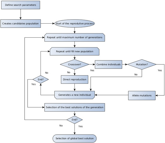
Figure 1.
Schematic representation of the GA algorithm.
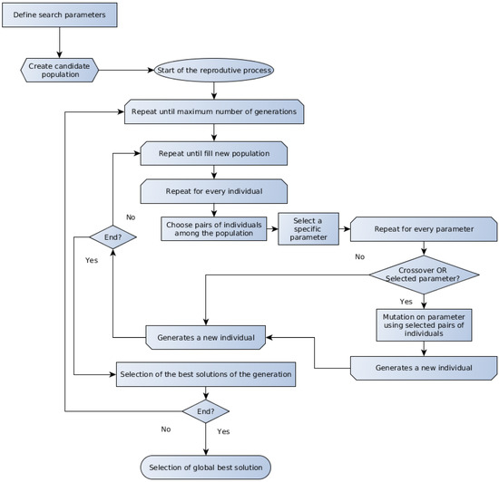
Figure 2.
Schematic representation of the DE algorithm.
2.4. DRTO of the Fermentative Process
For the DRTO of the ethanol production process, the optimization routine is triggered several times during the batch, with the feed rate as the manipulated variable trough the parametrization of the substrate input volumetric flow using the final ethanol productivity (g·h−1), as described in the following Section 2.5. The procedure for the DRTO execution is schematically presented in Figure 3, in which represent the optimal manipulated variable (substrate feed rate) input, d the disturbance in the stream fed in the fermenter, the output from process after the disturbance and u the value for the input variable. For the implementation of the DRTO routine, an in-house code developed using the Python computational language was utilized.
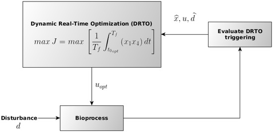
Figure 3.
Schematic representation of the procedure employed for the DRTO execution during the batch. Adapted from Ochoa et al. (2010) [29].
Several activation frequencies (or interval between optimization cycles) for the DRTO routine were evaluated, and an artificial disturbance in the form of a gaussian noise was introduced in the feed rate substrate concentration, as presented by several authors, such as Ochoa et al. Johansen, Tenny et al. [29,51,52], with a deviation of from the nominal value. It is important to emphasize that a productivity based objective function is appropriately for the control or optimization of a processes in which there is disturbance occurrence, instead of a defined operation point, as it can induce an unsatisfactory performance [29].
The parametrization of the feed rate was performed using a periodic function based in a non-linear mathematical expression based in cosinoidal terms, as presented in the work of Ochoa [15], an exponential and linear functions. The referred mathematical expressions are outlined in the following equations.
The mathematical expressions for the parametrization of the feed rate described in the Equations (14) and (15) exhibits important characteristics. Both functions represent smooth feed-rate profiles, avoiding the occurrence of inhibitory shocks due to substrate overfeeding, although this characteristic was not directly explored in the benchmark model employed in the present work, however the cosinoidal function is superior in this sense to the exponential one. However, it is important to mention that the exponential function has a smaller value for the degrees of freedom than the cosinoidal (4, instead of 7, respectively), what implies in a more compact set of variables to be determined by the optimization algorithm for each DRTO activation. In the other hand, the linear feed rate expression described in Equation (16) exhibit a non-smooth profile, although the expression has only 2 degrees of freedom.
2.5. Incidental Dynamic Optimization Problem
As previously described, in the DRTO a dynamic optimization problem (DOP) is triggered for each prediction horizon, as the CVP approach is employed for the parametrization of the manipulated variable (fermenter feed rate ) The DOP consists in the optimization of an objective function using the optimization algorithms, represented by Equation (17). The choice of the objective function represents a cardinal aspect of the DOP, and there is no consensus in the literature about which mathematical relation is more adequate for optimization studies, although the volumetric productivity is refereed to be more suited for batch culture processes in which the biocatalyst is not recovered after the process [53,54]. In this sense, this measure was utilized as the objective function in the present work, and it is mathematically outlined in Equation (17) , in terms of Equation (7) described earlier.
The objective function utilized represent the specific ethanol productivity g·h−1, in which the term represent the end time for the current prediction horizon, the final batch time, and represent the final ethanol concentration and fermenter volume in the end of the prediction horizon. Its important to mention that represent and additional degree of freedom for the DOP, as the optimization problem studied in the present work uses an open end-time concept. The constraints for the DRTO are presented in Table 2.
Table 2.
Constraints utilized for the resolution of the dynamic optimization problems.
Despite the fact that in the present work an in silico approach for ethanol production was employed, it is important to emphasize that the ethanol yield optimization has direct biological implications, as the manipulation of the substrate feed rate for the fed-batch process in study aims to maximize the excretion of ethanol concomitantly to the minimization of the inhibitory effect due to substrate and product accumulation. The conversion of the substrate in the biofuel is limited to the stoichiometric yield, theoretically limited to 0.511 g Ethanol/g sugars [55]. Several works was conducted in the determination of ethanol conversion from variate substrates, such as dried corn, with the approximate value of 90% [56] and switchgrass, with the value of approximately 80% [57]. Although the formulation of a mathematical model for the description of the microbial growth is limited in terms of the considerations made in its development, the applicability of in silico optimization is discussed in the works of Semple et al. Kumar and Maranas, Parambil and Sakar [58,59,60], among others.
For the parameter estimation for the feed rate function for each prediction horizon the stochastic optimization algorithms GA and DE were utilized. Both routines constitute in-house code developed using the Python computational language. The configurations employed for each algorithm are presented in Table 3 and Table 4, respectively.
Table 3.
Configuration employed in the genetic algorithm for the DOP of the DRTO.
Table 4.
Configuration employed in the differential evolution for the DOP of the DRTO.
2.6. Ethanol Production Simulation
The simulation of the ethanol production process was performed trough the integration of the ordinary differential system presented in Equations (1)–(6), with the initial values presented in Table 5. For this purpose, the odeint function was employed, provided by the odespy numeric library for the Python language [61], which act as a wrapper for the LSODA routine. This code switches between explicit and implicit integrators, depending of the differential system numeric stiffness, a mathematical property that is frequent for microbial growth simulation problems.
Table 5.
Initial values employed for the in silico ethanol production process variables.
3. Results and Discussions
In the following sections, the results obtained in the present work are presented. The effect of the interval for DRTO process triggering are evaluated. The dynamic profiles for each run of the simulated bioprocess are also depicted, and lastly, the comparison on the performance of each optimization algorithm for the incidental DOP is presented.
3.1. Effect of the Interval between Optimization Cycles and Parametrization Profile
The duration of the interval between the DRTO cycles represents an important aspect for the problem discussed in the present work, as it has implications in terms of the process sampling rate and the complexity of the underlying dynamical optimization problem. In Table 6, the effect of interval (INT, between 1, 2 and 4 h), optimization algorithm (ALG, GA or DE) and canonical profile for the feed rate parametrization (PROF, linear-lin-exponential-exp-or cosinoidal-cos) is presented. For the sake of clarification, the resultant profile is presented as INT/PROF/ALG. To minimize the inherent variability arousing from the stochasticity of the meta-heuristic algorithms, the result of every assay was obtained through the mean from 3 independent tests.
Table 6.
Results obtained for the DRTO in terms of the time interval between the optimization cycles (INT), optimization algorithm employed (ALG) and canonical profile for the feed rate parametrization (PROF).
The results presented in Table 6 show that the assays of number 5, 8, 9 and 16 (5/exp/GA, 4/cos/GA, 6/cos/GA and 2/cos/DE, respectively) exhibited the superior result in terms of productivity and batch time. The results also indicate that the reduced interval between the optimization cycles implies in a superior productivity. This could be explained for the simplicity of the microbial growth model, which does not account for deleterious effects such as overflow metabolism or inhibitory shocks for substrate feeding. It is worthwhile to mention that the obtained results, in terms of GA and DE comparison, corroborates with the empirically observed in the literature, as the genetic algorithm exhibits in general more result variability than the differential evolution [50,62]. Also, it is important to notice that for both algorithms the exponential parametrization of the feed rate exhibited larger variaton among the results (expressed in terms of its standard deviation), especially for the assays with higher time interval between the optimization studies. However, its is important to notice that the cosinoidal feed rate profile, as an inherently smooth function, possess the notable property of avoiding inhibitory shocks due to substrate feeding, although this characteristic was not explored in the present study, as mentioned before.
Is important to mention that the results obtained for the batch duration time (presented in Table 6), which represent an additional degree of freedom for the underlying sequential DOPs, exhibit notable results, being in totality equal of inferior to h, approximately. The occurrence of shorter batches with appreciable productivity indexes (such as the assays 5, 8, 9 and 16), represent a relevant result for the present study, as it implies in either in a superior net profit for the process. Those results demonstrate the capacity of the DRTO algorithm to optimize the process output, despite the disturbance in one of the inputs, the concentration of the substrate feed rate.
The variability in the results for the different parametrization for the GA has shown suggestive statistical evidences that the corresponding results are in fact different. In Figure 4, the confidence intervals for each assay are presented, representing imagetically the difference in the order of magnitude of the specific ethanol productivity (g·h−1) variability for both algorithms.
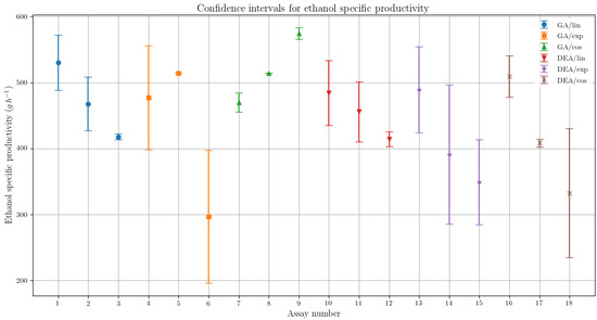
Figure 4.
Confidence interval comparison between the assays for the specific ethanol productivity, presenting the variability respective to each optimization algorithm and feed rate parametrization.
In terms of the the batch durations presented in Table 6, their results showed lower dispersion when compared with the specific ethanol productivity, as aforementioned. The comparison between confidence intervals obtained for the fermentation time is presented in Figure 5.
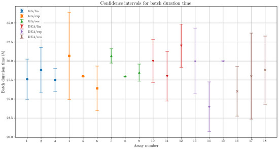
Figure 5.
Confidence interval comparison between the assays for the batch duration time, presenting the variability respective to each optimization algorithm and feed rate parametrization.
In Figure 5, is possible to observe that the GA algorithm exhibited less variability than the DE, as similarly noted for the specific ethanol production results. This fact corroborates with the characteristics observed empirically for the differential evolution, as aforementioned.
In order to evaluate the significance of the parameters employed in bioethanol production optimization using the DRTO, two ANOVA tests were performed for the GA and DE, with the interval between optimization cycles (or DRTO frequency) (INT) and fermenter feed rate parametrization profile (PROF) as the analyzed factors. In Table 7 and Table 8, the results are presented.
Table 7.
Analysis of variance (ANOVA) table for the ethanol productivity, using the GA as the optimization algorithm. The terms SS, df, MS represent the summation of the squared variations, number of degrees of freedom and mean squared variation, respectively.
Table 8.
Analysis of variance (ANOVA) table for the ethanol productivity, using the DE as the optimization algorithm. The terms SS, df, MS represent the summation of the squared variations, number of degrees of freedom and mean squared variation, respectively.
The results presented in Table 7 and Table 8 suggests that for a confidence level of 95%, it is not possible to reject the hypothesis that both time intervals between optimization cycles and parametrization profile for the fermenter feed rate are significant for the results employing GA as the optimization algorithm. However, for the results regarding the utilization of DE as the optimization algorithm, only the parametrization profile has shown to be significant for the productivity results. The interaction between the analyzed factors, in terms of bioethanol production process productivity and batch time duration results in terms of the DRTO frequency, for each parametrization profile, is presented in Figure 6 and Figure 7.
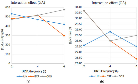
Figure 6.
Interactions graph for the ethanol productivity (a) and batch duration time (b) with the parametrization profile (LIN—linear, EXP—exponential and COS—cosinoidal) and DRTO interval (2, 4 or h) as the analyzed factors, using GA as the optimization algorithm.
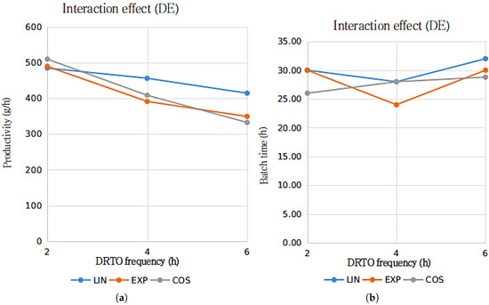
Figure 7.
Interactions graph for the ethanol productivity (a) and batch duration time (b) with the parametrization profile (LIN—linear, EXP—exponential and COS—cosinoidal) and DRTO interval (2, 4 or h) as the analyzed factors, using DE as the optimization algorithm.
The results presented in Figure 6 and Figure 7 suggests that for bioethanol productivity, there is an substantial interaction between the DRTO frequency and parametrization profile for the results using the GA as the optimization algorithm, whilst the interaction between the analyzed factor for the results using DE as the optimization algorithm is significantly inferior. In terms of the batch duration time, the results are similar, although the interactions regarding the GA as the optimization algorithm indicate that the interaction are notably more pronounced for the exponential parametrization profile.
In order to compare the bioethanol productivity results obtained in the DRTO assays (presented in Table 6) in terms of the parametrization profiles for the fermenter feed rate for each optimization algorithm, a pairwise t-test comparison with the Bonferonni correction procedure was employed, using a confidence level of 95%. The p-values obtained in the tests are presented in Table 9. In the referred table, the terms INT1, INT2 and INT3 were used to represent the interval between the DRTO cycles (2, 4 and h, respectively), with the aim to improve the readability of the results.
Table 9.
Results of p-values for the pairwise t-test with Bonferonni correction, in terms of the different parametrization profiles, using GA as the optimization algorithm (a) and DE (b).
The results presented in Table 9 indicate that, for a confidence level of 95%, for several assays there is no evidence that the different parametrization profiles implies in a increment in bioethanol productivity. In order to facilitate the readability of the results obtained, in Table 10 the positive results (indicating that the parametrization profiles differ in terms of the final bioethanol productivity) are highlighted.
Table 10.
Interpretation for the results of the pairwise t-test with Bonferonni correction, in terms of the different parametrization profiles, using GA as the optimization algorithm (a) and DE (b). The positive results are marked as an asterisk (*), and the negative with a dot (•).
The obtained results presented in Table 10 indicate that for a confidence level of 95%, for the assays with the interval between optimization cycles of h using the GA as the optimization algorithm exhibited significant differences between the parametrization profiles. In terms of the results using the DE for the optimization, only the exponential profile exhibited significant difference. It is important to emphasize that, considering the evidence suggested by the comparison of confidence intervals in Figure 4, the aforementioned numerical results of the pairwise t-tests can be justified by the variability in the results, which is expressive for some assays, causing the variation between parametrization profiles to be treated as random errors.
3.2. Dynamic Profiles for the Specific Productivity of In-Silico Ethanol Production Process
The dynamic growth profiles for the ethanol production process (g·h−1) are presented in Figure 8, Figure 9, Figure 10 and Figure 11, comparing the profiles obtained with the assays that exhibited superior results in terms of ethanol specific productivity, respectively 5 (4 h/GA/exp), 8 (4 h/GA/cos), 9 (6 h/GA/cos) and 16 (2 h/DE/cos). In the profiles, the growth is represented in terms of the concentration of substrate, ethanol and cellular biomass during the batch. The total batch time employed for each assay correspond to the mean value determined in the optimization studies, presented in Table 6.
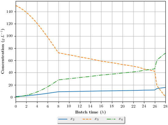
Figure 8.
Growth profile for the assay of number 5 (4 h/GA/exp—4 h interval between DRTO cycles, GA as the optimization algorithm and exponential feed rate parametrization), in terms of the concentration of cellular biomass (), substrate () and ethanol () during the batch.
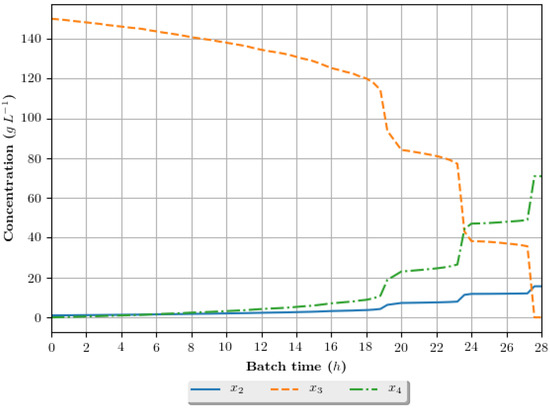
Figure 9.
Growth profile for the assay of number 8 (4 h/GA/cos—4 h interval between DRTO cycles, GA as the optimization algorithm and cosinoidal feed rate parametrization), in terms of the concentration of cellular biomass (), substrate () and ethanol () during the batch.
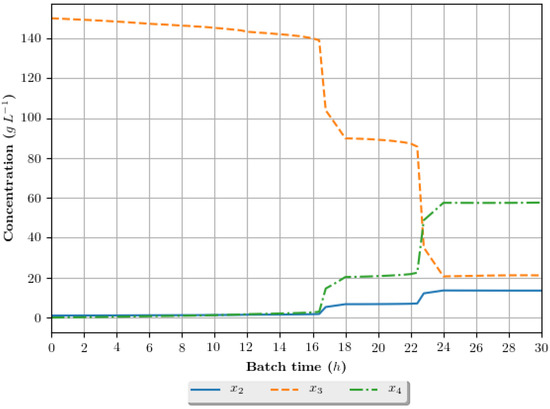
Figure 10.
Growth profile for the assay of number 9 (6 h/GA/cos—6 h interval between DRTO cycles, GA as the optimization algorithm and coisinoidal feed rate parametrization), in terms of the concentration of cellular biomass (), substrate () and ethanol () during the batch.
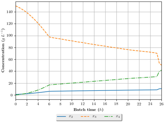
Figure 11.
Growth profile for the assay of number 16 (2 h/DE/cos—2 h interval between DRTO cycles, DE as the optimization algorithm and cosinoidal feed rate parametrization), in terms of the concentration of cellular biomass (), substrate () and ethanol () during the batch.
3.3. Comparison between the Optimization Algorithms
Despite the aforementioned relatively small divergence in the results obtained, it is possible to observe that the standard deviation of DE is superior to the GA, in terms of both productivity and batch time. This indicates that despite the fact that both algorithms are essentially evolutionary methods, the GA exhibited a better convergence rate than the DE for the problem in discussion.
In order to evaluate the performance of both algorithms in terms of its intrinsic properties, a trial run was performed for each one using an open-loop feed rate optimization concept, as presented by several authors, such as Banga et al. Ochoa, Rocha et al. [14,15,18,50], for the initial configurations presented in Table 5, and a fixed batch time of 50, 54, and h, using the cosinoidal parametrization for the feed rate (14). The results are presented in Table 11, from the information presented in the work of Ochoa [15].
Table 11.
Results obtained for the open-loop optimization, comparing between GA and DE optimization algorithms.
The results presented in Table 11 indicate that the GA exhibited a superior performance than the DE, although the difference between both was diminished significantly for the longer batches (e.g., when comparing h and h fermentations). Also, it is important to mention that both algorithms (GA and DE) employed in the present work has exhibited better performance, in terms of the final value of the objective function (mass of ethanol in the fermenter after the fermentation time) than some results presented in the literature, except for the assay with h of batch duration.
In order to compare the optimization algorithm, a pairwise t-test comparison with the Bonferonni correction procedure was employed, using a confidence level of 95%. The p-values obtained in the tests are presented in Table 12. In the referred table, the terms , and were used to represent the interval between the DRTO cycles (2, 4 and h, respectively), with the aim to improve the readability of the results. In this sense, the positive results (indicating that the optimization algorithms differ in terms of the final bioethanol productivity) were highlighted.
Table 12.
Pairwise t-test with Bonferonni correction, in terms of the optimization algorithms employed in the DRTO study, GA and DE. The positive results are marked as an asterisk (*), and the negative with a dot (•).
The results presented in Table 12 indicate that for a confidence level of 95%, there is statistical evidence that the results obtained using the GA algorithm were superior to those obtained with the DE, only for the assay with h as the interval between the DRTO cycles and the cosinoidal parametrization profile, corresponding to the assays 11 and 17 in Table 6. However, it is important to emphasize that similarly to the results for the pairwise t-test for the parametrization profiles, presented in Table 9, the expressive variability of some assays allied to the conservative nature of the Bonferonni correction could lead to the consideration of the variation between the productivity results using different optimization algorithms as a result of inherent data discrepancy. This high variability can be justified by the number of replicates performed for each DRTO assay (in the present work, a number of three was employed), and the increment of the number of runs could reduce the data dispersion.
4. Conclusions
In this work, a study concerning the utilization of a DRTO approach for a benchmark ethanol in silico production process was conducted, using the substrate feed rate as the controlled variable and employing an artificial noise in the process input of substrate concentration in this stream, with the open batch end time, using the GA and DE for the resolution of the underlying optimization problems. The GA has exhibited superior convergence rates than the DE, and less variability in terms of the resultant specific ethanol productivity and batch time duration. High specific productivity results were obtained (superior to 574 g·h−1 ), with relatively short batch times (inferior to h). The open-loop optimization study results, used to evaluate the isolated performance of the developed GA and DE algorithm shows that the algorithms developed in this work have notable performance, obtaining values very close or superior to what was obtained by several authors.
The comparison of confidence intervals for the results using the different optimization algorithms and parametrization profiles in terms of the productivity results suggests that the GA exhibited superior performance than DE, as well as the cosinoidal parametrization when compared to the exponential and linear profiles. However, the results of the statistical analysis of the influence of different parametrization in the productivity results pointed out that for the GA, the only the cosinoidal exhibited significant difference to the other profiles, using h as the DRTO frequency; for the DE, the exponential profile exhibited significant superior results to the linear. Similarly, the results for the analysis for comparison of the optimization algorithms indicates that that the results for both are statistically equivalent, except for the result using the GA and an interval of h for the DRTO cycles. This discrepancy between the qualitative and numerical analysis can be justified due to the expressive variability observed in the assay results, allied to the conservative nature of the statistical test employed for the comparison.
Author Contributions
Cid Marcos Gonçalves Andrade guided the research; Hanniel Ferreira Sarmento de Freitas implemented the software employed in the calculations, performed the simulations and wrote the paper; Cid Marcos Gonçalves Andrade and José Eduardo Olivo proofread the paper.
Conflicts of Interest
The authors declare no conflict of interest.
References
- Panwar, N.; Kaushik, S.; Kothari, S. Role of renewable energy sources in environmental protection: A review. Renew. Sustain. Energy Rev. 2011, 15, 1513–1524. [Google Scholar] [CrossRef]
- Vanholme, B.; Desmet, T.; Ronsse, F.; Rabaey, K.; Van Breusegem, F.; De Mey, M.; Soetaert, W.; Boerjan, W. Towards a carbon-negative sustainable bio-based economy. Front. Plant Sci. 2013, 4. [Google Scholar] [CrossRef] [PubMed]
- Demirbas, A. Political, economic and environmental impacts of biofuels: A review. Appl. Energy 2009, 86, S108–S117. [Google Scholar] [CrossRef]
- Demirbas, A.H.; Demirbas, I. Importance of rural bioenergy for developing countries. Energy Convers. Manag. 2007, 48, 2386–2398. [Google Scholar] [CrossRef]
- Koçar, G.; Civaş, N. An overview of biofuels from energy crops: Current status and future prospects. Renew. Sustain. Energy Rev. 2013, 28, 900–916. [Google Scholar] [CrossRef]
- Balat, M. Production of bioethanol from lignocellulosic materials via the biochemical pathway: A review. Energy Convers. Manag. 2011, 52, 858–875. [Google Scholar] [CrossRef]
- Popp, J.; Lakner, Z.; Harangi-Rákos, M.; Fári, M. The effect of bioenergy expansion: Food, energy, and environment. Renew. Sustain. Energy Rev. 2014, 32, 559–578. [Google Scholar] [CrossRef]
- Mayer, F.D.; Feris, L.A.; Marcilio, N.R.; Hoffmann, R. Why small-scale fuel ethanol production in Brazil does not take off? Renew. Sustain. Energy Rev. 2015, 43, 687–701. [Google Scholar] [CrossRef]
- Vohra, M.; Manwar, J.; Manmode, R.; Padgilwar, S.; Patil, S. Bioethanol production: Feedstock and current technologies. J. Environ. Chem. Eng. 2014, 2, 573–584. [Google Scholar] [CrossRef]
- Baeyens, J.; Kang, Q.; Appels, L.; Dewil, R.; Lv, Y.; Tan, T. Challenges and opportunities in improving the production of bio-ethanol. Prog. Energy Combust. Sci. 2015, 47, 60–88. [Google Scholar] [CrossRef]
- Chen, H.; Zhou, D.; Luo, G.; Zhang, S.; Chen, J. Macroalgae for biofuels production: Progress and perspectives. Renew. Sustain. Energy Rev. 2015, 47, 427–437. [Google Scholar] [CrossRef]
- Wang, Y.; Chu, J.; Zhuang, Y.; Wang, Y.; Xia, J.; Zhang, S. Industrial bioprocess control and optimization in the context of systems biotechnology. Biotechnol. Adv. 2009, 27, 989–995. [Google Scholar] [CrossRef] [PubMed]
- Gadkar, K.G.; Mehra, S.; Gomes, J. On-line adaptation of neural networks for bioprocess control. Comput. Chem. Eng. 2005, 29, 1047–1057. [Google Scholar] [CrossRef]
- Banga, J.R.; Balsa-Canto, E.; Moles, C.G.; Alonso, A.A. Dynamic optimization of bioprocesses: Efficient and robust numerical strategies. J. Biotechnol. 2005, 117, 407–419. [Google Scholar] [CrossRef] [PubMed]
- Ochoa, S. A new approach for finding smooth optimal feeding profiles in fed-batch fermentations. Biochem. Eng. J. 2016, 105, 177–188. [Google Scholar] [CrossRef]
- Rani, K.Y.; Rao, V.R. Control of fermenters—A review. Bioprocess Eng. 1999, 21, 77–88. [Google Scholar] [CrossRef]
- Pimentel, G.A.; Benavides, M.; Dewasme, L.; Coutinho, D.; Wouwer, A.V. An Observer-based Robust Control Strategy for Overflow Metabolism Cultures in Fed-Batch Bioreactors. IFAC-PapersOnLine 2015, 48, 1081–1086. [Google Scholar] [CrossRef]
- Rocha, M.; Mendes, R.; Rocha, O.; Rocha, I.; Ferreira, E.C. Optimization of fed-batch fermentation processes with bio-inspired algorithms. Exp. Syst. Appl. 2014, 41, 2186–2195. [Google Scholar] [CrossRef]
- Şendrescu, D. Nonlinear model predictive control of a depollution bioprocess. In Proceedings of the 2011 Third Pacific-Asia Conference on Circuits, Communications and System (PACCS), Wuhan, China, 17–18 July 2011; pp. 1–4. [Google Scholar]
- Şendrescu, D.; Popescu, D.; Petre, E.; Bobaşu, E.; Selişteanu, D. Nonlinear model predictive control of a lipase production bioprocess. In Proceedings of the 2011 12th International Carpathian Control Conference (ICCC), Velke Karlovice, Czech Republic, 25–28 May 2011; pp. 337–341. [Google Scholar]
- Spadiut, O.; Rittmann, S.; Dietzsch, C.; Herwig, C. Dynamic process conditions in bioprocess development. Eng. Life Sci. 2013, 13, 88–101. [Google Scholar] [CrossRef]
- Spadiut, O.; Herwig, C. Dynamics in bioprocess development for Pichia pastoris. Bioengineered 2014, 5, 401–404. [Google Scholar] [CrossRef] [PubMed]
- Del Rio-Chanona, E.A.; Zhang, D.; Vassiliadis, V.S. Model-based real-time optimisation of a fed-batch cyanobacterial hydrogen production process using economic model predictive control strategy. Chem. Eng. Sci. 2016, 142, 289–298. [Google Scholar] [CrossRef]
- Wang, S.; Ma, Z.; Zhang, T.; Bao, M.; Su, H. Optimization and modeling of biohydrogen production by mixed bacterial cultures from raw cassava starch. Front. Chem. Sci. Eng. 2017, 11, 100–106. [Google Scholar] [CrossRef]
- Sridevi, K.; Sivaraman, E.; Mullai, P. Back propagation neural network modelling of biodegradation and fermentative biohydrogen production using distillery wastewater in a hybrid upflow anaerobic sludge blanket reactor. Bioresour. Technol. 2014, 165, 233–240. [Google Scholar] [CrossRef] [PubMed]
- Kana, E.G.; Oloke, J.; Lateef, A.; Adesiyan, M. Modeling and optimization of biogas production on saw dust and other co-substrates using artificial neural network and genetic algorithm. Renew. Energy 2012, 46, 276–281. [Google Scholar] [CrossRef]
- Enitan, A.M.; Adeyemo, J.; Swalaha, F.M.; Kumari, S.; Bux, F. Optimization of biogas generation using anaerobic digestion models and computational intelligence approaches. Rev. Chem. Eng. 2017, 33, 309–335. [Google Scholar] [CrossRef]
- Jacob, S.; Banerjee, R. Modeling and optimization of anaerobic codigestion of potato waste and aquatic weed by response surface methodology and artificial neural network coupled genetic algorithm. Bioresour. Technol. 2016, 214, 386–395. [Google Scholar] [CrossRef] [PubMed]
- Ochoa, S.; Repke, J.U.; Wozny, G. Integrating real-time optimization and control for optimal operation: Application to the bio-ethanol process. Biochem. Eng. J. 2010, 53, 18–25. [Google Scholar] [CrossRef]
- Gernaey, K.V.; Lantz, A.E.; Tufvesson, P.; Woodley, J.M.; Sin, G. Application of mechanistic models to fermentation and biocatalysis for next-generation processes. Trends Biotechnol. 2010, 28, 346–354. [Google Scholar] [CrossRef] [PubMed]
- Fernandes, R.L.; Bodla, V.K.; Carlquist, M.; Heins, A.L.; Lantz, A.E.; Sin, G.; Gernaey, K.V. Applying mechanistic models in bioprocess development. In Measurement, Monitoring, Modelling and Control of Bioprocesses; Mandenius, C.F., Titchener-Hooker, N.J., Eds.; Springer: Berlin, Germany, 2013; pp. 137–166. [Google Scholar]
- Hong, J. Optimal substrate feeding policy for a fed batch fermentation with substrate and product inhibition kinetics. Biotechnol. Bioeng. 1986, 28, 1421–1431. [Google Scholar] [CrossRef] [PubMed]
- Wechselberger, P.; Sagmeister, P.; Engelking, H.; Schmidt, T.; Wenger, J.; Herwig, C. Efficient feeding profile optimization for recombinant protein production using physiological information. Bioprocess Biosyst. Eng. 2012, 35, 1637–1649. [Google Scholar] [CrossRef] [PubMed]
- Ye, J.; Xu, H.; Feng, E.; Xiu, Z. Optimization of a fed-batch bioreactor for 1, 3-propanediol production using hybrid nonlinear optimal control. J. Process Control 2014, 24, 1556–1569. [Google Scholar] [CrossRef]
- Henes, B.; Sonnleitner, B. Controlled fed-batch by tracking the maximal culture capacity. J. Biotechnol. 2007, 132, 118–126. [Google Scholar] [CrossRef] [PubMed]
- Croughan, M.S.; Konstantinov, K.B.; Cooney, C. The future of industrial bioprocessing: Batch or continuous? Biotechnol. Bioeng. 2015, 112, 648–651. [Google Scholar] [CrossRef] [PubMed]
- Zydney, A.L. Perspectives on integrated continuous bioprocessing—Opportunities and challenges. Curr. Opin. Chem. Eng. 2015, 10, 8–13. [Google Scholar] [CrossRef]
- Kawohl, M.; Heine, T.; King, R. Model based estimation and optimal control of fed-batch fermentation processes for the production of antibiotics. Chem. Eng. Process. Process Intensif. 2007, 46, 1223–1241. [Google Scholar] [CrossRef]
- Banga, J.R. Optimization in computational systems biology. BMC Syst. Biol. 2008, 2, 47. [Google Scholar] [CrossRef] [PubMed]
- Apel, A.C.; Weuster-Botz, D. Engineering solutions for open microalgae mass cultivation and realistic indoor simulation of outdoor environments. Bioprocess Biosyst. Eng. 2015, 38, 995–1008. [Google Scholar] [CrossRef] [PubMed]
- Santo, G.E.; Pedro, A.; Oppolzer, D.; Bonifácio, M.; Queiroz, J.; Silva, F.; Passarinha, L. Development of fed-batch profiles for efficient biosynthesis of catechol-O-methyltransferase. Biotechnol. Rep. 2014, 3, 34–41. [Google Scholar] [CrossRef] [PubMed]
- Helbig, A.; Abel, O.; Marquardt, W. Structural concepts for optimization based control of transient processes. In Nonlinear Model Predictive Control; Springer: Berlin, Germany, 2000; pp. 295–311. [Google Scholar]
- Würth, L.; Rawlings, J.B.; Marquardt, W. Economic dynamic real-time optimization and nonlinear model-predictive control on infinite horizons. IFAC Proc. Vol. 2009, 42, 219–224. [Google Scholar] [CrossRef]
- Biegler, L.; Yang, X.; Fischer, G. Advances in sensitivity-based nonlinear model predictive control and dynamic real-time optimization. J. Process Control 2015, 30, 104–116. [Google Scholar] [CrossRef]
- Liu, P.; Li, G.; Liu, X.; Zhang, Z. Novel non-uniform adaptive grid refinement control parameterization approach for biochemical processes optimization. Biochem. Eng. J. 2016, 111, 63–74. [Google Scholar] [CrossRef]
- Balsa-Canto, E.; Banga, J.R.; Egea, J.A.; Fernandez-Villaverde, A.; de Hijas-Liste, G. Global optimization in systems biology: Stochastic methods and their applications. Adv. Syst. Biol. 2012, 736, 409–424. [Google Scholar]
- Penas, D.; Banga, J.; González, P.; Doallo, R. Enhanced parallel Differential Evolution algorithm for problems in computational systems biology. Appl. Soft Comput. 2015, 33, 86–99. [Google Scholar] [CrossRef]
- Ohenoja, M.; Leiviskä, K. Validation of genetic algorithm results in a fuel cell model. Int. J. Hydrogen Energy 2010, 35, 12618–12625. [Google Scholar] [CrossRef]
- Moles, C.G.; Mendes, P.; Banga, J.R. Parameter estimation in biochemical pathways: A comparison of global optimization methods. Genome Res. 2003, 13, 2467–2474. [Google Scholar] [CrossRef] [PubMed]
- Rocha, M.; Pinto, J.P.; Rocha, I.; Ferreira, E.C. Evaluating evolutionary algorithms and differential evolution for the online optimization of fermentation processes. In Proceedings of the 5th European Conference on Evolutionary Computation, Machine Learning and Data Mining in Bioinformatics, Valencia, Spain, 11–13 April 2007; Springer: Berlin, Germany, 2007; pp. 236–246. [Google Scholar]
- Johansen, T.A. Toward dependable embedded model predictive control. IEEE Syst. J. 2015, 10. [Google Scholar] [CrossRef]
- Tenny, M.J.; Rawlings, J.B.; Wright, S.J. Closed-loop behavior of nonlinear model predictive control. AIChE J. 2004, 50, 2142–2154. [Google Scholar] [CrossRef]
- Maurer, M.; Kühleitner, M.; Gasser, B.; Mattanovich, D. Versatile modeling and optimization of fed batch processes for the production of secreted heterologous proteins with Pichia pastoris. Microb. Cell Fact. 2006, 5, 37. [Google Scholar] [CrossRef] [PubMed]
- Illanes, A.; Wilson, L.; Vera, C. Problem Solving in Enzyme Biocatalysis; John Wiley & Sons: New York, NY, USA, 2013. [Google Scholar]
- Krishnan, M.S.; Ho, N.W.; Tsao, G.T. Fermentation kinetics of ethanol production from glucose and xylose by recombinant Saccharomyces 1400 (pLNH33). Appl. Biochem. Biotechnol. 1999, 78, 373–388. [Google Scholar] [CrossRef]
- Patzek, T.W. A statistical analysis of the theoretical yield of ethanol from corn starch. Nat. Resour. Res. 2006, 15, 205–212. [Google Scholar] [CrossRef]
- Vogel, K.P.; Dien, B.S.; Jung, H.G.; Casler, M.D.; Masterson, S.D.; Mitchell, R.B. Quantifying actual and theoretical ethanol yields for switchgrass strains using NIRS analyses. BioEnergy Res. 2011, 4, 96–110. [Google Scholar] [CrossRef]
- Semple, J.L.; Woolridge, N.; Lumsden, C.J. In vitro, in vivo, in silico: Computational systems in tissue engineering and regenerative medicine. Tissue Eng. 2005, 11, 341–356. [Google Scholar] [CrossRef] [PubMed]
- Kumar, V.S.; Maranas, C.D. GrowMatch: An automated method for reconciling in silico/in vivo growth predictions. PLoS Comput. Biol. 2009, 5, e1000308. [Google Scholar] [CrossRef] [PubMed]
- Parambil, L.K.; Sarkar, D. In silico analysis of bioethanol overproduction by genetically modified microorganisms in coculture fermentation. Biotechnol. Res. Int. 2015, 2015. [Google Scholar] [CrossRef] [PubMed]
- Langtangen, H.P.; Wang, L. Odespy Software Package, 2015. Available online: https://github.com/hplgit/odespy (acessed on 6 July 2017).
- Hegerty, B.; Hung, C.C.; Kasprak, K. A comparative study on differential evolution and genetic algorithms for some combinatorial problems. In Proceedings of the 8th Mexican International Conference on Artificial Intelligence, Guanajuato, Mexico, 9–13 November 2009; pp. 9–13. [Google Scholar]
- Chen, C.T.; Hwang, C. Optimal on-off control for fed-batch fermentation processes. Ind. Eng. Chem. Res. 1990, 29, 1869–1875. [Google Scholar] [CrossRef]
- Jayaraman, V.; Kulkarni, B.; Gupta, K.; Rajesh, J.; Kusumaker, H. Dynamic Optimization of Fed-Batch Bioreactors Using the Ant Algorithm. Biotechnol. Prog. 2001, 17, 81–88. [Google Scholar] [CrossRef] [PubMed]
- Banga, J.R.; Alonso, A.A.; Singh, R.P. Stochastic dynamic optimization of batch and semicontinuous bioprocesses. Biotechnol. Prog. 1997, 13, 326–335. [Google Scholar] [CrossRef]


© 2017 by the authors. Licensee MDPI, Basel, Switzerland. This article is an open access article distributed under the terms and conditions of the Creative Commons Attribution (CC BY) license (http://creativecommons.org/licenses/by/4.0/).