1. Introduction
In a regulated environment, the customers have to pay the set price as established by the utility company. In this environment the power flow from the generation to consumer meter is entirely controlled by the vertically integrated utility. Recently, the power system has encountered real changes and has also been operating in a deregulated environment. The vertically coordinated systems are being rebuilt and unbundled into generation, transmission, and distribution entities. In this environment, customers will get reliable services, more choices, and need to pay less amounts for the consumption of electricity in the competitive market. In addition to these, privatization and functional separation of existing power system entities are the stands behind the causes of the deregulated power industry [
1]. In this new environment, the traditional centralized system is lost and leads to the formation of new companies participating in the generation. This made the generating companies more dependent on decision-making tools for the analysis of all the possible investment and selling options in the present competitive environment [
2].
Traditional unified power system networks are taking energy from high voltage (HV) levels and sending it to low voltage (LV) level distribution network (DN), but in the era of the deregulated environment, there will be a need of lively distribution network management, from central to many distribution networks. In this kind of network, there will be more distributed generations (DG’s) in the system along with latest advanced ideas [
3]. Along these lines, overhead distribution frameworks are fundamentally arranged in a radial way to make simple inherent components of the system assurance, for example, coordination and lessening of short out streams and decreasing hardware costs [
4]. Low adaptability and dependability for the functioning of radial distribution networks (RDNs) cause those frameworks to be developed through the sectionalizing switches (SS) [
5]. By varying the condition of the SS, i.e., opening or closing, the network is being reconfigured, and the function of the network is also enhanced [
6]. Modification in the topology of any distribution network reduces the system’s loss, enhances the system’s voltage profile (VP), and restores the power supply. Along these lines, SS are utilized for fault segregation in addition to the reconfiguration [
7,
8].
These days, distribution networks that are being affected by expanding the addition of DGs, which are constantly utilized as a part of the transmission network [
9]. Hereafter, DG got to be one of the applicable parameters in the assessment of network reconfiguration [
10]. The incorporation of DG in any distribution network influences the operation of this DN in different courses [
11]. An intriguing issue that is identified with DG is the loss allocation (LA) issue, which turns out to be essential to the presentation of utility rivalry [
12].
Section 2 provides some of the recent research works done in this field.
Section 3 describes the suggested technique, and
Section 4 shows the simulated outcomes using the proposed technique along with discussion. Finally, in
Section 5, the results are concluded, followed by references.
2. Related Works
Oliveira et al. [
13] had presented a simulator based on the graphic for DNs with network reconfiguration and earmark of losses applications. They used current summation backward-forward technique taking into account DG to form a power flow algorithm for solving reconfiguration problem. They implemented and did a comparison of four LA methods, which were “Zbus, Direct Loss Coefficient, Substitution and Marginal Loss Coefficient” on a 32 bus system. From the comparison of these methods, it was found that the Zbus method had a better performance and was simple to implement, while “Substitution and Marginal Loss Coefficient methods” required an adjustment factor.
Savier and Das [
14] proposed an LA technique for the deregulated environment before and after reconfiguration. The method was formed in a quadratic way and stood on the determination of two different parts of current in each branch. The suggested algorithm was based on multi-objective optimization in a fuzzy environment. For this, three objectives were examined and were modelled in a fuzzy framework. The 69 node balanced test system results revealed that there was a reduction in real power losses with reconfiguration and LA to most of the consumers were reduced, but it was also observed that LA to some consumers may increase, resulting in more payment after reconfiguration. From these observations, they found that the allocation of real power loss to each consumer was affected by the objectives that were considered for network reconfiguration.
Chandramohan et al. [
15] suggested a technique for minimizing the operating cost of balanced RDNs in a deregulated environment. They reconfigured the network using “non-dominated sorting genetic algorithm (NSGA)”. They minimized the operating cost and maximized the operating reliability so that the operating constraints were satisfied. They used the related formulas available in literature. They tested their method on balanced 33 node and 69 node RDNs.
Atanasovski and Taleski [
16] had proposed a “Power Summation Method” to allocate loss in RDNs with DG. The suggested approach is branch oriented, which was formed from the backward sweep power summation method without any kind of approximations and assumptions. They treated active and reactive loads as positive, and DGs were representing negative loads. They decomposed the branch losses to node related components, which made their suggested method simple and efficient for DN. The suggested method is applied to balanced 32 node RDN and results were correlated with the “Branch Current Decomposition Loss Allocation (BCDLA)” method and “Marginal Loss Coefficients (MLC)” method.
Savier and Das [
17] had given a method to allocate real power loss in RDN in a deregulated environment. They compared their suggested “Exact Method” with two algorithms that are available in the literature; first was depended on each consumer load demand called “Pro rata algorithm” and second was “Quadratic loss allocation” scheme, those identified the two different components of current in each branch. LA to each consumer was carried out and the suggested method was tested on balanced 30 node RDN.
Ghofrani-Jahromi et al. [
18] had presented an LA technique in RDNs depending on the outcomes of power flow and considering the active and reactive power flow through the lines. They considered three steps. The power loss designated to all of the nodes starting from the nodes having generation greater than their load computed in the earlier step. At the same time, the power loss that is designated to the loads associated with each node is achieved. In the next step, the LA starts from the sink nodes, i.e., nodes having a load greater than their generation. In the last step, the execution of normalization was done. Their suggested method was tested taking 17 node and 69 node RDNs.
Jagtap and Khatod [
19] had offered a method for LA to DGs and consumers those who were associated with RDNs in the emancipated market. The prime motives of that paper were focused on the nonlinear alliance between the flow of power and losses, revisions of system losses due to the variation of voltage, and benefaction of DG to system’s loss. The technique presented in [
13] had been used in LA. The application of the method was once again limited to 28 node and 33 node balanced RDNs.
Jagtap and Khatod [
20] had proposed a technique for the LA in balanced RDNs using diverse models of DG and loads in a deregulated environment. Without assuming and approximating anything, they derived a straight relation between active and reactive power flow and its losses. “Power summation algorithm” (PSA) was used to derive approximate expressions/relations for power flow of network and any cross term was avoided. A network dependent branch oriented technique was used to allocate the losses among the members of the network. The LA to any DG/load at different nodes was carried out using backward sweep network diminution algorithm. The LA in two different RDNs (nine node and 33 node) had been performed in the presence of different types of DG and load models.
Sharma and Abhyankar [
21] presented an efficient method of loss allocation with Shapley value and network laws. They had provided a solution with a cooperative game theory approach. They used Shapley value for balanced radial and weekly meshed distribution system to solve the analytical solution provided by the proposed method. They used the network data and power flow solutions without any assumptions in their proposed method. They had given the results with different setups of network topologies, DG output levels rivalled their result by two other Shapely value based balanced test systems. They had shown that the Shapely value based LA had given the best result in comparison to the other methods reported.
Kaur and Ghosh [
22] presented a method to reconfigure unbalanced distribution networks (UDNs) in the fuzzy environment using the Firefly algorithm in a regulated environment. They also suggested a load flow method for the solution of UDNs. They had also rigorously discussed different available methods of reconfiguration in a deregulated environment. Their suggested method was tested on 19 and 25 node UDNs. The concluded results were compared with the outcomes attained by “Genetic algorithm (GA), Artificial Bee Colony (ABC) algorithm, Particle Swarm Optimization (PSO) algorithm and Genetic algorithm-Particle Swarm Optimization (GA-PSO) algorithm”, keeping the objective function unaltered.
3. Proposed Methodology for Network Reconfiguration and LA in UDN
The formations of UDNs might be changed with manual or programmed switching application in order to decrease power loss, expand network security, and improve power quality. Despite the fact that the principal mission of network reconfiguration is to decline the losses of the system in a deregulated environment, the reconfiguration deliberates the objectives that are identified with expanding the benefits of an organization, for example, operational cost minimization and reliability maximization. Likewise, in the deregulated environment, the losses are assigned to various purchasers in the network. In this work, the effect of network reconfiguration, the integration of DG and capacitor in the reconfigured network, and the impact of LA in UDNs in both the regulated and deregulated environments are presented. The network reconfiguration problem is defined as a fuzzy based multi-objective problem. For optimization of the network, the Firefly optimization algorithm is utilized, which augments the fuzzy based objective function. The proposed formulation of problem considers the accompanying viewpoints:
LA of 13 node UDN and comparison of outcomes obtained by proposed method and that of by [
12].
LA of base network (25 node UDN) and its reconfigured network in regulated environment.
DG and capacitor have been placed in reconfigured network using Loss Sensitivity Factor (LSF) and Bacteria foraging optimization algorithm (BFOA).
LA of the network after placement of DG and capacitor.
The above steps are also carried for deregulated environment. Network reconfiguration in the deregulated environment using the established Fuzzy-Firefly algorithm [
22] is carried out. The details of Firefly algorithm are available in [
22]. The well-established optimization equations available in [
23,
24,
25] used by [
15] also have been used in unbalanced systems incorporating suitable changes. The same optimization algorithm i.e., Firefly has been used to obtain loss allocation.
3.1. LA in UDN
The three phase currents are recognized by
and
, however,
is the neutral current. For the purpose of notation, the vector
is the phase current vector, and the vector
includes the complex voltages in the phase terminals of the genetic node k. The total losses can be computed as the sum of losses due to each physical current path
Or utilizing the primitive impedance matrix .
Or utilizing the 3 × 3 primitive impedance matrix
ZabcAccording to the impedances matrix symmetry, Equation (2) can be altered applying the real part operator only to the impedance in order to extract its resistive components. So, the overall branch losses can be computed through the real part of impedance matrix Zabc.
The formulation of Equation (2) leads to the loss partitioning. Here, it is suggested to estimate the loss partitioning by utilizing Equation (5). By representing with ⊗ the component by-component vector product, the loss partition vector
denoted to three phases
a,
b, and
c in the equivalent
matrix representation of the branch is considered as
The total loss in Equation (5) corresponds to the sum of the components of the vector . The real part operator is required in Equation (6) because of the effect of the off-diagonal components of the matrix Rabc. It is no longer needed in Equation (5), as all of the imaginary parts are mutually compensated in the sum.
3.2. Network Reconfiguration of UDN in Deregulated Environment
Any UDN consists of two types of switch, known as normally open switch (tie-line switch) and normally closed switch (sectionalizing switch). By closing the tie-line switches and opening sectionalizing switches, the arrangement of the distribution network can be modified. The loss minimization may not be optimal with the opening and closing of improper switches. Hence, the selection of switches is most vital to get the optimal network, which gives a maximum loss reduction and superior VP. Any predetermined reason identifies the function of a specific configuration. For example, a configuration with maximum loss reduction and superior VP is always expected. The aim to reconfigure any network is to reduce loss, expand reliability indices, use of a maximum number of switches, and cut down the working cost of the system. The intelligent algorithm can be used to compute the objective function having multiple variables. The consequence of any objective can be determined by the weighting elements. It is not required to install any additional instruments to take care of network issues; those can be solely done by reconfiguring the network. Any network having ‘n’ number of open or closed switches will have ‘2n’ number of arrangements. Hence, it is not feasible to think about all states of reconfiguring the network. During reconfiguring the network, the following limitations are considered:
All of the network buses must be limited.
Summation of net load and net losses must tally with the generation and should be neither equal nor exceed the capacity of the network.
The final structure of the network must be radial.
Bus voltages should be within the limits.
The reconfiguration problem becomes a complex optimization problem due to its huge solution space and a number of constraints. The cost of the network in the deregulated environment should be paid the highest attention in comparison to any general network in the regulated environment, and hence the objective function in a deregulated environment becomes entirely different. This paper considers multi-objective optimization for reconfiguring the network. In this proposed methodology, for the case of reconfiguration in a regulated environment, reducing the power loss, reducing the bus voltage deviance, and load equalizing done by the feeders are considered as the objectives and fuzzified, as mentioned in [
22]. The objective function for network reconfiguration in a regulated environment is available in [
22] and presented below.
The fitness function is deliberated in Equation (7) is maximized during the optimization procedure to acquire the best well-matched configuration. This operator has numerous benefits. For instance, if any membership function of each objective reaches the value of zero, λFm is allocated to a value of zero. Additionally, this function delivers correct information as about how making this algorithm achieving an ideal state, namely a value of 1. This objective function is utilized as the fitness function. As the network cost is more significant in the case of the deregulated environment when compared to the traditional network, the deregulated environment has a different objective function. In the deregulated environment, the main objective is to improve the benefits for the company. Here, two objectives are considered for the deregulated environment, such as operational cost minimization and reliability maximization.
In this work, the fireflies move with the values of β = 1, γ = 0.75, and α = 0.25 are considered where β, γ, and α are the intensity or attractiveness of the firefly’s flashing light, light absorption coefficient of a given medium, and randomization parameter, . The number of firefly population is taken as 100 and the maximum number of iterations is selected as 150.
3.3. Minimization of Operational Cost
There are two parts of the net operating cost. The cost due to real power loss is considered as operation cost at first that can be reduced by reducing the losses in the distribution network. The cost due to real power loss is equal to A1 × PS, where A1 is the coefficient for the price of real power and its unit is $/kW and a net loss of system’s active power (PS) in kW. The second component is the reactive power cost, as procured with the distribution network. The cost component can be decreased if the system’s reactive power loss is decreased. The second component is represented by A2 × QS, where A2 represents the coefficient of price in $/kVAr and QS represents the reactive power that is consumed by the distribution network from the transmission system connected to it. The Operating Cost (C) is represented by Equation (8).
The operational cost minimization index is given by
where
C0 indicates the initial operating cost before reconfiguration and
Cm indicates the operating cost after reconfiguration in the
mth system. The fuzzy satisfaction degree of the operating cost objective function is computed by exploiting the membership function, as represented by the fuzzy domain, which is expressed as follows:
where,
XCmin and
XCmax are the lower and upper limits of
XCm index, correspondingly. To compute the
XCmin and
XCmax, consider both the best and worst system configuration of the operating cost.
Cm for the system’s best configuration is the least value of the operating cost and for the system’s worst configuration is anticipated to be equal to the operating cost of the initial configuration.
3.4. Reliability Optimization
The crucial principle for the optimal operation of any distribution network is the operational reliability. For the optimization process, the operational reliability is considered. The reliability is calibrated by computing failure cost. The interruption of the customer’s activity is occurring by the service disruption to every customer. The total service interruption duration function is represented as Customer Interruption Cost (CIC), which boosts with time and the amount of the cost is piecewise conversely commensurate to the time. Here, Customer Interruption Cost is the measured cost averaged through time. Let the
mth bus is being supplied power by the link, which is the nth element of the system. Let
λn failures/year be the average failure rate of the nth element of the system and
rn minutes/year taken as “average failure duration” acknowledging records for considerable years. If
Lm is the load of the
mth bus, the “Cost of Service Interruption” for the consumer at the same bus is expressed by Equation (11)
In Equation (11), rm is the entire service break period at the mth bus seeing all of the other breaks, which will be described later. The load is considered as the set of elements that are supplied to the mth bus. The indices generate a set k(m). Using Equation (12) “total interruption cost” for a service break at the same bus can be computed.
Rearranging Equation (12),
Defining and
λm represents “average interruption rate” and
rm represents “average interruption duration”, those are foreseen by a consumer at the
mth bus contemplating the failures of all components those committed to “service interruption” on the same bus.
ICm in Equation (13) is known as “value based reliability index”, which is assessed by probabilistic study, probable financial loss in a year through the service break at the same bus. For a specific configuration “Total Interruption Cost (TIC)” can be expressed as in Equation (14).
where
N is the total number of buses.
The total interruption cost index is given by
where
TIC0 indicates the initial total interruption cost before reconfiguration and
TICm indicates the total interruption cost after reconfiguration in the
mth system. The fuzzy satisfaction degree for the total interruption costs is computed by exploiting the membership function as represented by the fuzzy domain, which is represented by Equation (16).
where,
XTmin and
XTmax are the lower and upper limits of
XTm index, correspondingly. To compute the
XTmin and
XTmax, consider both the best and worst system configuration of the operating cost.
Tm is the minimum value of the entire interruption cost for the best system configuration and for the worst system configuration it is anticipated to be equal to the total interruption cost of the initial configuration. Finally, for reconfiguration in a deregulated environment, there are two objectives, namely, optimize “operational cost minimization and operational reliability maximization”, as obtained by curtailing TIC of customer after merging two objectives
Equation (17) is regarded as the “fitness function” to be maximized through the process of optimization so that the best well-matched configuration in the deregulated environment is obtained. The optimal network reconfiguration at the deregulated environment is obtained by the established “Fuzzy-Firefly algorithm”, as used in [
22] for the regulated environment.
3.5. DG and Capacitor Placement
The optimum location of DG and capacitor in UDN is decided by Equation (18) [
26], which presents the mathematical expression of “Loss Sensitivity Factor” (LSF) of three phase UDN. LSF is arranged in descending order and the highest value is considered for placement of DG and capacitor.
where
K,
I,
br,
n,
, and
R are the voltage ratio, current, branch number, bus number, phase, and resistance.
The DG (Type-I i.e., delivers only active power) is placed at first to the most sensitive node and its size is determined by Bacteria foraging optimization algorithm (BFOA). The details of BFOA are available in [
27]. The objective function in this case is given in Equation (19).
Next, LSF is found once again. The capacitor is placed to the most sensitive node and its size is determined by Bacteria foraging optimization algorithm (BFOA). Here, DG is placed at first because the available LSF is related to resistance of the network. The proposed LSF-BFOA method for the placement of DG and capacitor is to be compared with the LSF-GA method. The details of Genetic algorithm (GA) are available in [
28].
4. Outcomes and Discussion
In this section, the efficiency of the suggested algorithm is tested severely on diverse types of UDN. In MATLAB working platform the proposed method of LA is implemented on 13 node UDN at first to check its performance when compared to other existing techniques, and then finally implemented on 25 UDN. The system configuration is mentioned as follows:
SYSTEM CONFIGURATION:
Operating System (OS): Windows 8
RAM Capacity: 4 GB
Processor model: Intel Core i3-3210
Frequency of the system: 3.19 GHz
MATLAB 2013a
4.1. 13-Node UDN
The proposed method of LA is implemented on IEEE 13 node UDN having 20 equally distributed load. The network configuration and other parameters are available in [
12].
Table 1 shows the outcomes obtained by the proposed method and that of by [
12].
The proposed method gives the loss allocation in more uniform way as compared to [
12].
4.2. 25-Node UDN in Regulated Environment
A 25 node UDN is considered as a common test case having 4.16 kV, 30 MVA as base values. It consists of switches with three tie lines and the total load is 3.239 + j2.393 MVA. Network data are presented in [
29]. Initial configuration of the network and final configuration after network reconfiguration are available in [
22]. The detailed results for the base case and after network reconfiguration are also available in [
22].
The voltage levels and LA to each consumer for base network and reconfigured network in a regulated environment are given in
Table 2. The node number is for voltage level and branch number for loss allocation. This configuration has 25 nodes and 24 branches. The values in italics are for loss allocation.
The DG and capacitor are integrated to the reconfigured UDN. The location DG and Capacitor are obtained by the LSF. Their sizes are determined by BFOA and Genetic Algorithm (GA) and the outcomes of both cases are presented in
Table 3.
The DG and capacitor are integrated into the reconfigured network for three phase to reduce the losses and also the LA after the integration of DG and capacitor is carried out. The results before and after the integration of DG and capacitor in the reconfigured network are presented in
Table 4.
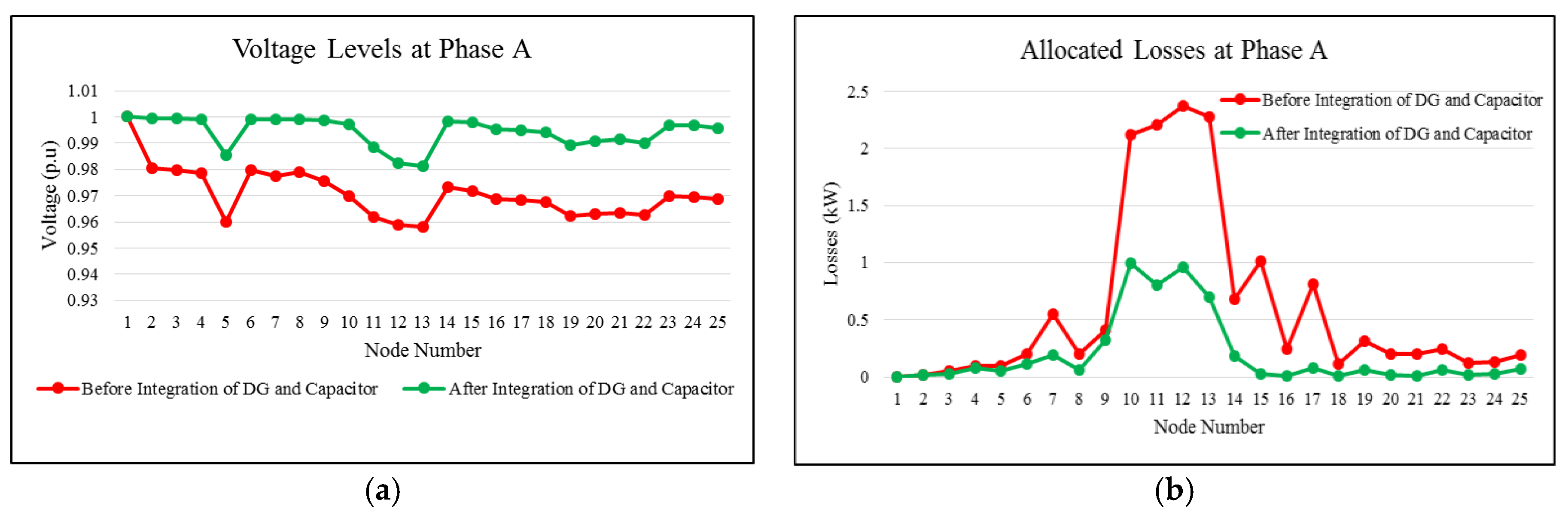
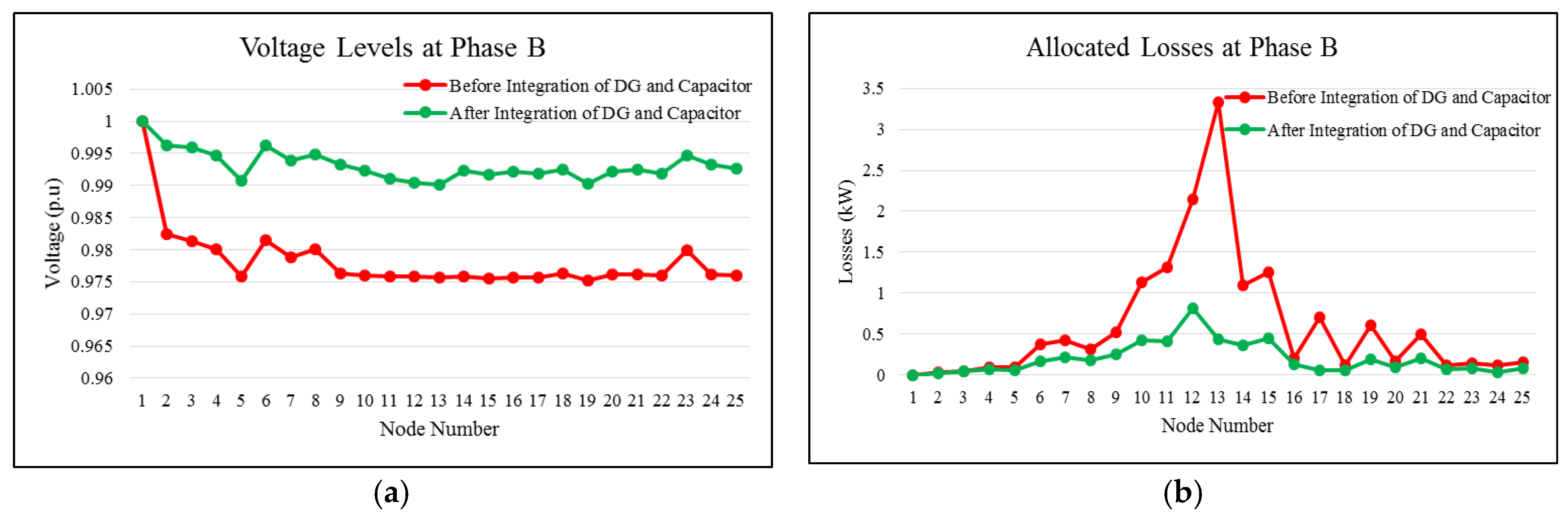
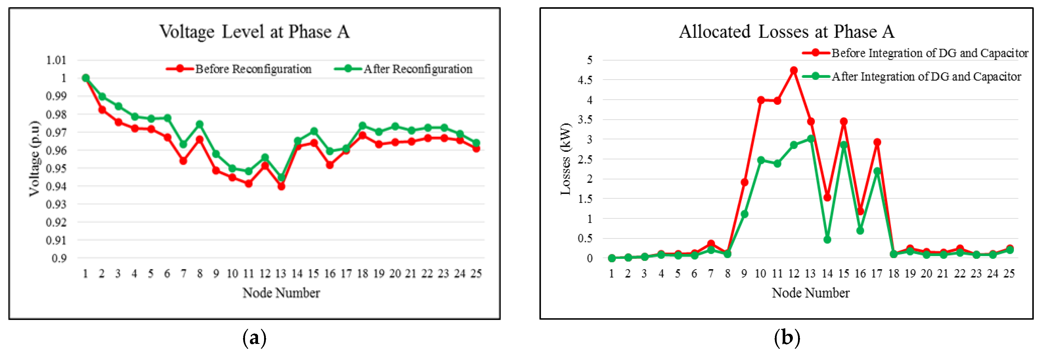
The results of LA before and after integration of DG and capacitor in the reconfigured network, as well as the voltage levels of the system are presented in
Table 5. The node number is for voltage level and branch number for loss allocation. This configuration has 25 nodes and 24 branches. The values in italics are for loss allocation.
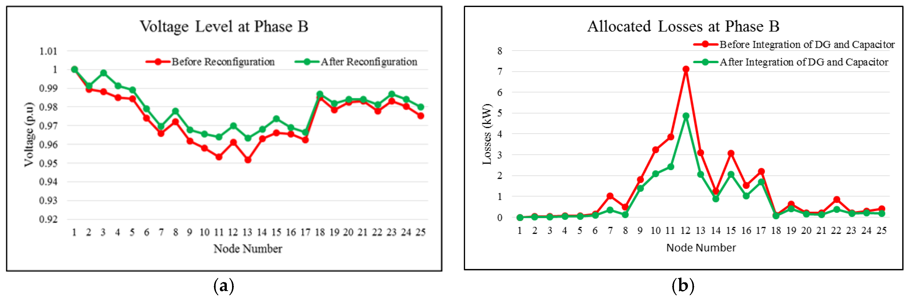
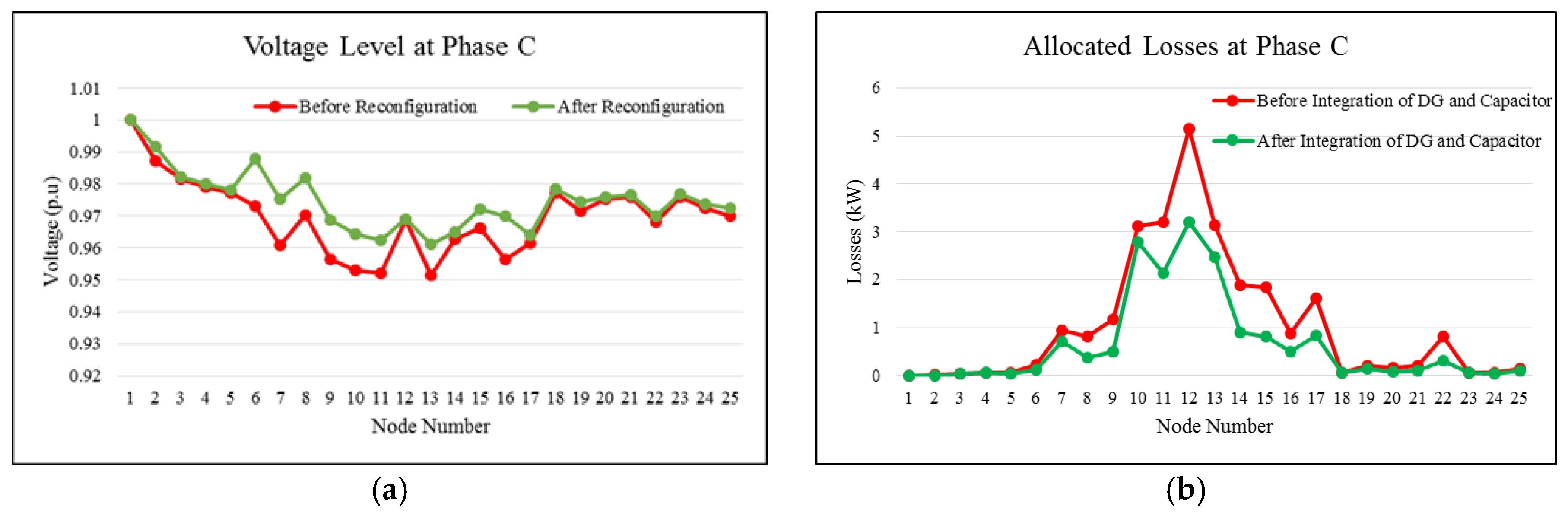
Figure 1a,
Figure 2a, and
Figure 3a show the representation of voltage levels of the Phases A–C, respectively, before and after the integration of DG and capacitor in the reconfigured network.
Figure 1b,
Figure 2b, and
Figure 3b show the LA of the Phases A–C, respectively, before and after the integration of DG and capacitor in the reconfigured network.
4.3. 25-Node UDN in Deregulated Environment
In a deregulated environment, data of equipment failure is given in
Table 6 [
15], and “the customer interruption cost” in
$ per minute per kW are given in
Table 7 [
15] and K
1 = 5
$/kW and K
2 = 2
$/kVAr [
15], respectively and the customers considered are of commercial type load.
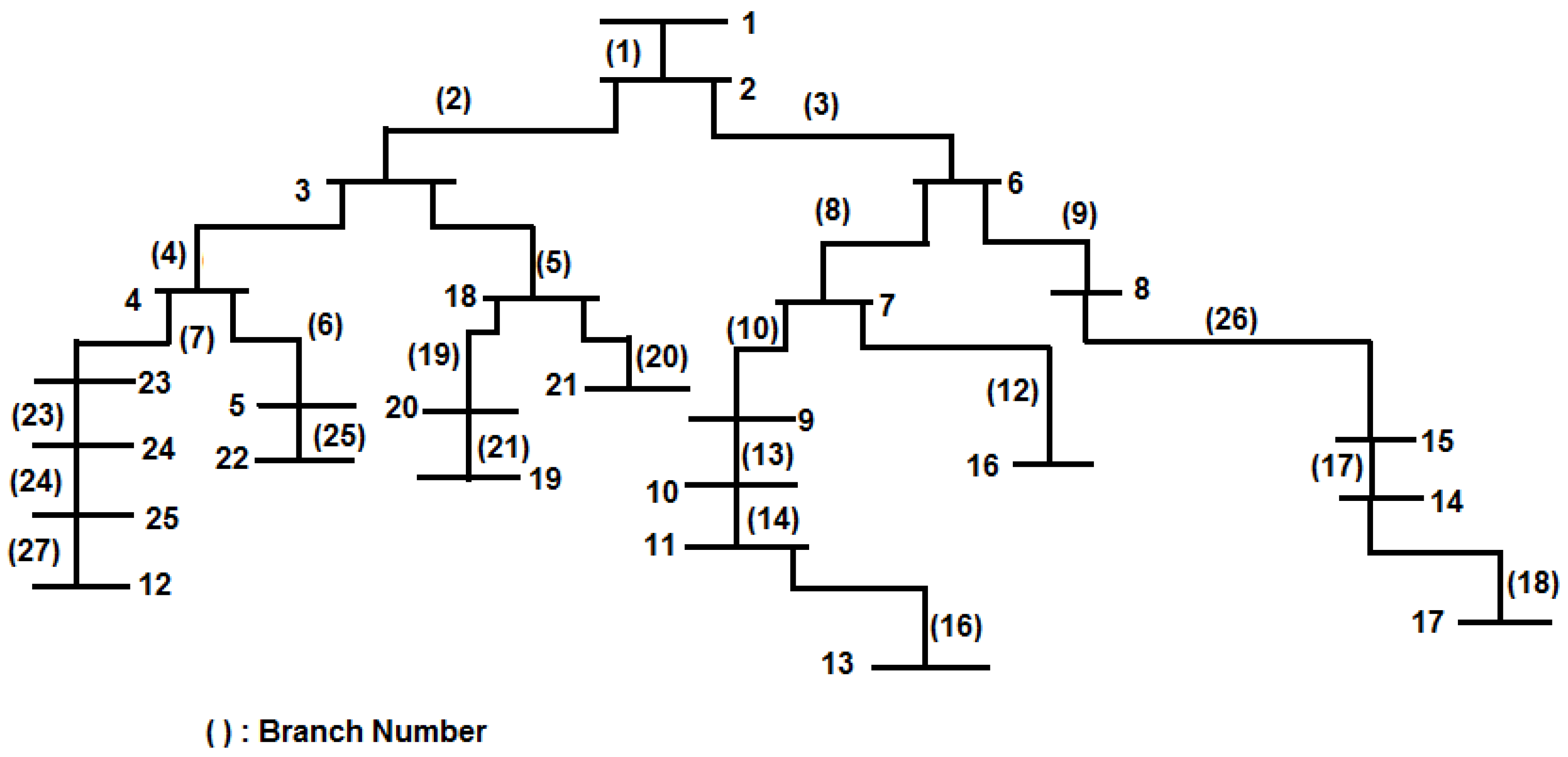
The 25 node UDN is reconfigured in the deregulated environment and the final configuration is shown in
Figure 4. The simulation results of this network before and after network reconfiguration is shown in
Table 8.
The voltage levels and LA in the deregulated environment before and after network reconfiguration are shown in
Table 9. The node number is for voltage level and branch number for loss allocation. This configuration has 25 nodes and 24 branches. The values in italics are for loss allocation.
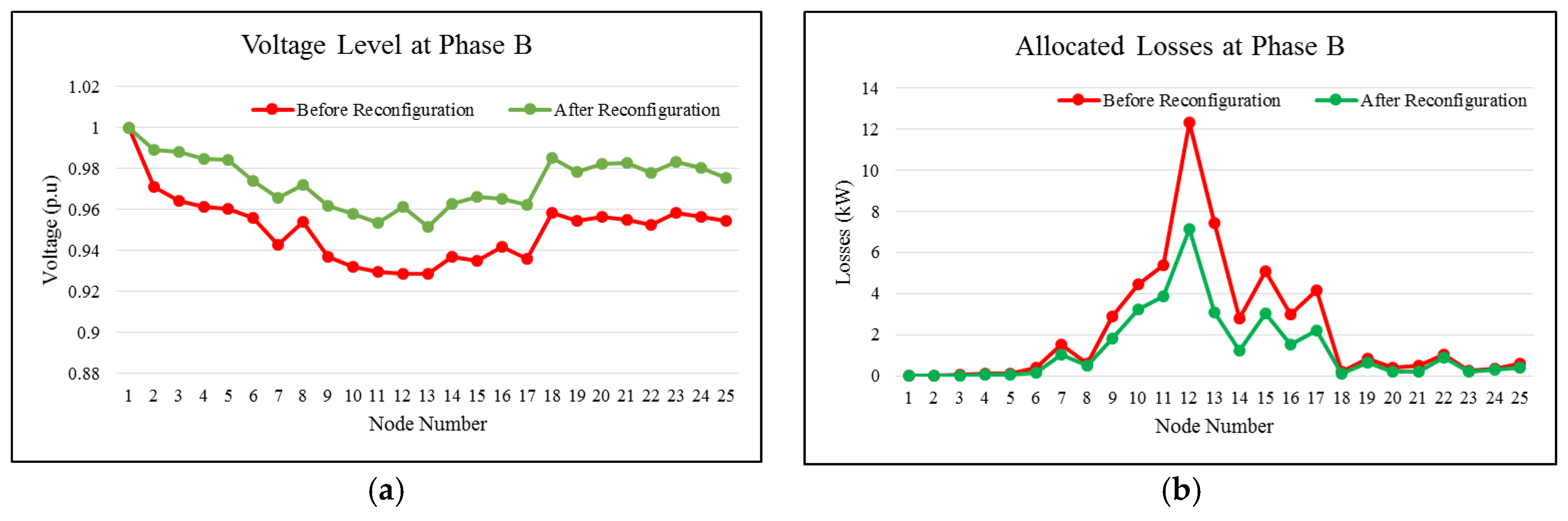
Figure 5a,
Figure 6a, and
Figure 7a show the representation of voltage levels of base and reconfigured networks for the Phases A–C, respectively.
Figure 5b,
Figure 6b, and
Figure 7b show the loss allocated base and reconfigured networks for the Phases A–C, respectively. The voltage level has been improved after network reconfiguration. Since the losses are reduced after network reconfiguration, the amount of allocated loss is also reduced.
The DG and capacitor are being integrated into the reconfigured network in a deregulated environment to further reduce the losses. The results before and after the integration of DG and capacitor in the reconfigured network are shown in
Table 10.
The voltage levels and LA in the deregulated environment before and after integration of DG and capacitor are shown in
Table 11. The node number is for voltage level and branch number for loss allocation. This configuration has 25 nodes and 24 branches. The values in italics are for loss allocation.
Figure 8a,
Figure 9a, and
Figure 10a show the representation of voltage levels of the Phases A–C, respectively, before and after integration of DG and capacitor in the reconfigured network.
Figure 8b,
Figure 9b, and
Figure 10b show the LA of the Phases A–C, respectively, before and after integration of DG and capacitor in the reconfigured network.
From these results, the losses are allocated before and after network reconfiguration in regulated and deregulated environments, as well as we have analyzed LA after the integration of DG and capacitor in the reconfigured network in both of the environments. Nowadays, in most of the existing research, the main focus was on balanced DNs but in the proposed method we have concentrated on unbalanced DN. In the already existing works, the focus is either on network reconfiguration, DG placement, or capacitor placement. Here, in our work, we are combining the advantage of network reconfiguration, DG, and capacitor placement, and we also have shown the impact of these in LA in both the regulated and deregulated environment.


