3.1. The Results of Time Difference Correlation Coefficient
Each value of the time difference term will have a corresponding result of the correlation coefficient, so a series of correlation coefficients can be obtained by changing the value of the time difference term. For the high-frequency monthly data, each change of one month in the length of time difference will be able to obtain a new correlation coefficient value. According to a series of findings, a shorter time difference term does not reflect the real time difference relationship because sometimes the maximum correlation coefficient appears in the longer time difference term. On the other hand, a longer time difference term does not necessarily lead to more accurate results. When changing the value of the time difference term, the whole time series data needs to be moved to meet the computational requirements. In this case, the data length of the original time series changes, which will be shorter with a larger time difference term. Further, the representativeness of the result of the time difference correlation coefficient decreases as the data length becomes shorter. Taking into account the above factors, 18 months are selected as the maximum value of the time difference term. In addition, we assume that the time difference relationship remains stable under different time difference terms with the maximum value of 18 months.
For each sector, positive and negative values of the time difference term with the maximum value of 18 months will generate 36 results of the correlation coefficient. Coupled with the result of synchronization, a total of 37 sets of results can be obtained, including the correlation coefficient and the corresponding number of time difference terms.
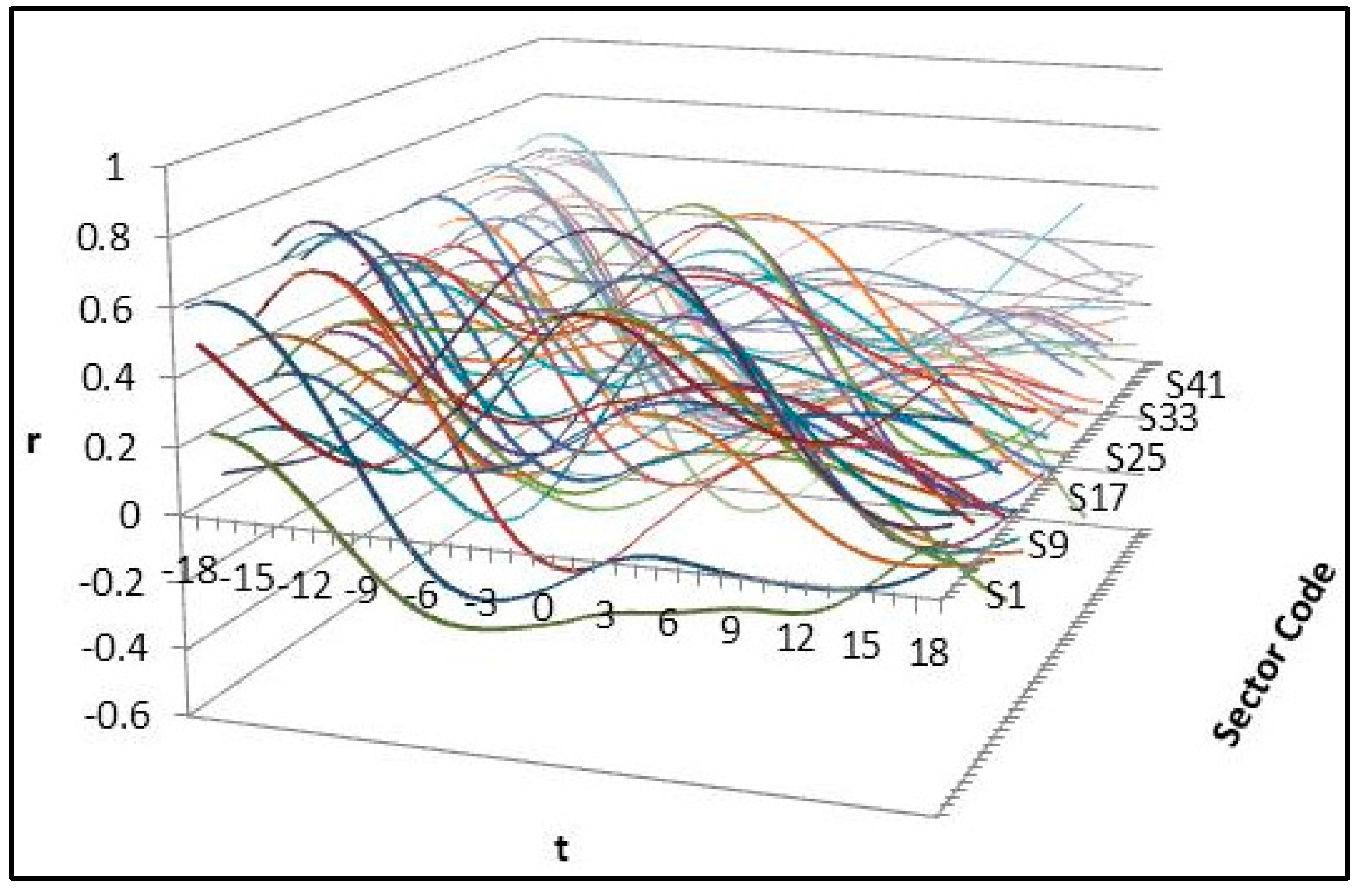
Figure 3 shows the results of time difference correlation coefficient of all 46 sectors. Each line represents the time difference results of one sector that compares with the basic series. It reflects the correlation relationship between the electricity consumption growth of a sector and economic growth under different leading or lagging months. In
Figure 3, the
t-axis represents the number of time difference terms, ranging from −18 to 18. Negative values represent a leading relationship, while positive values represent a lagging relationship, with zero for a synchronization relationship. The r-axis represents the value of the correlation coefficient, whose maximum absolute value is not greater than 1. A positive value indicates a positive correlation between sectoral electricity consumption growth and economic growth, and a value closer to 1 indicates a higher correlation between the two series. In contrast, a negative value shows a negative correlation between sectoral electricity consumption growth and economic growth. A value of 1 means that the two series are identical, a value of −1 indicates the two series are exactly the opposite, and a value of 0 indicates that the two sequences are completely unrelated.
For each sector, there are 37 correlation coefficients between electricity consumption growth and economic growth. Since the maximum value of the correlation coefficient is considered to reflect the correlation relationship under the certain terms, a set of data reflecting the time difference relationship can be obtained including the largest correlation coefficient and the corresponding time difference term. Thus, the results of the time difference correlation coefficient between electricity consumption growth of all 46 sectors and economic growth can be obtained, as shown in
Table 1. The correlation coefficient varies from a minimum of 0.096 to a maximum of 0.865, with all values positive, indicating a strong or weak positive correlation between the electricity consumption growth of all sectors and economic growth. S4, the sector of mining and processing of ferrous metal ores, has the maximum correlation coefficient with the time difference relationship lagging two months. S27, the sector of comprehensive use of waste resources, has the minimum correlation coefficient with the time difference relationship lagging seven months. The correlation coefficient close to zero indicates a very weak correlation between electricity consumption growth of S27 and economic growth.
3.2. The Results of Kullback-Leibler Divergence
The same as the correlation coefficient results, each value of the time difference term will have a corresponding result of KL divergence. For the same monthly data, a series of correlation coefficients can be obtained by changing the value of the time difference term. For comparison and consistency analysis, 18 months are still selected as the maximum value of the time difference term.
For each sector, 36 results of KL divergence will be obtained with both positive and negative values of the time difference term. Coupled with the result of synchronization, a total of 37 sets of results can be obtained, including the KL divergence and the corresponding number of time difference terms.
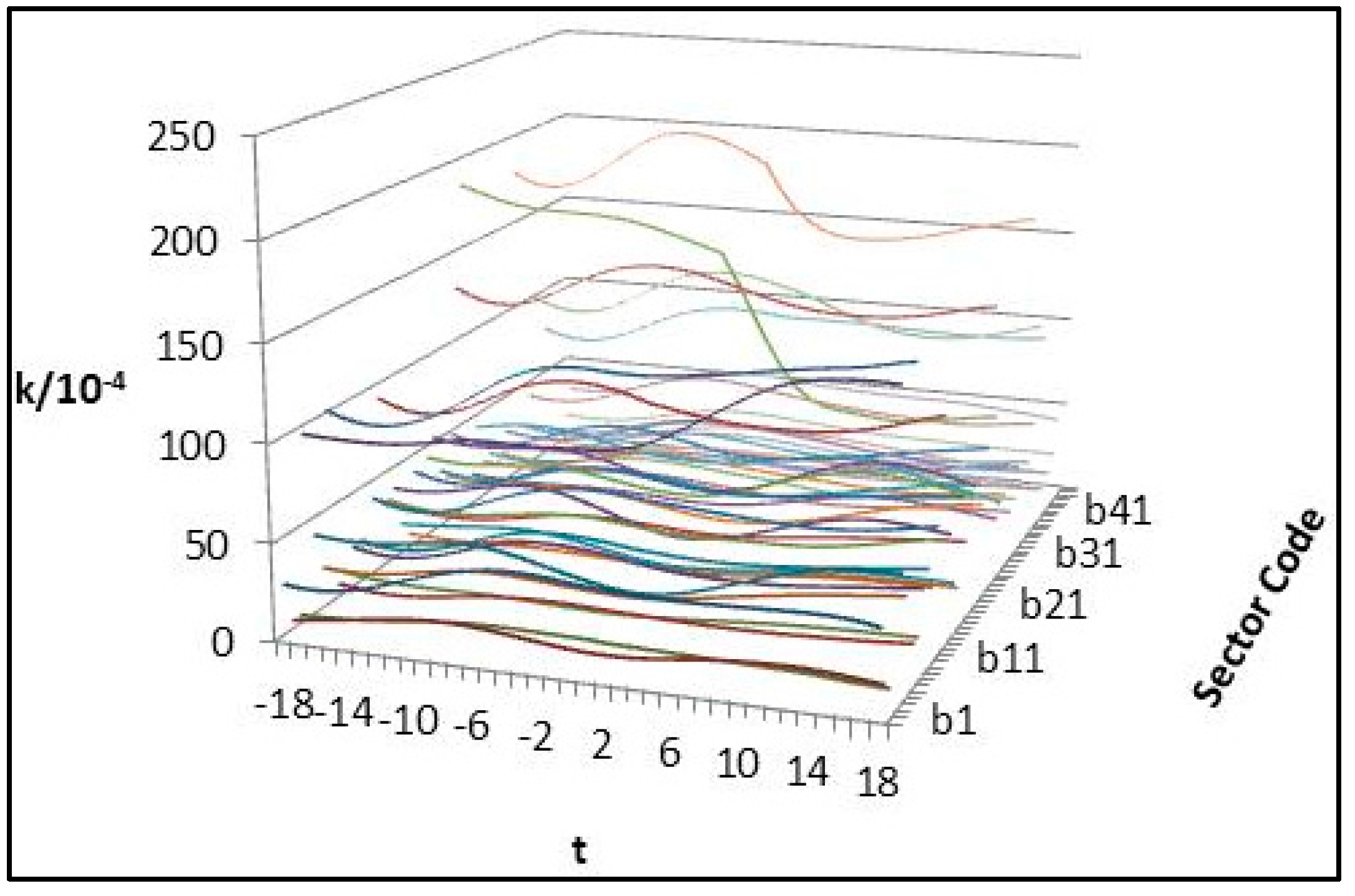
Figure 4 shows the results of KL divergence of all 46 sectors. Each line represents the KL divergence results of one sector reflecting the approximate degree of probability distribution between the electricity consumption growth of a sector and economic growth under different leading or lagging months. In
Figure 4, the t-axis represents the number of time difference terms, ranging from −18 to 18. Negative values represent a leading relationship, while positive values represent a lagging relationship, and zero for a synchronization relationship. The value of the
k-axis, which represents KL divergence, is always non-negative and takes the value of zero if and only if two series are equal. According to the definition of KL divergence, a smaller value means two series are more similar. A value closer to 0 indicates that the probability distribution of sectoral electricity consumption growth is more similar to the probability distribution of economic growth. When the KL divergence between two series takes the value of 0, they are completely consistent in terms of the probability distribution.
A total of 37 results of KL divergence can be obtained for each sector. Since the minimum value of KL divergence is considered to reflect the similarity degree under the certain terms, a set of data including the minimum KL divergence and the corresponding time difference term can be selected to reflect the similarity relationship. Thus, the results of KL divergence between electricity consumption growth of all 46 sectors and economic growth can be obtained, as shown in
Table 2. Since the calculated values of KL divergence were too small, the data given in the table were the results expanded by 10,000 times. The KL divergence varies from a minimum of 6.355 to a maximum of 156.639, indicating different degrees of similarity between the electricity consumption growth of all sectors and economic growth. S40, the sector of real estate, has the minimum KL divergence with the time difference relationship leading seventeen months. S36, the sector of software and information technology services, has the maximum KL divergence with the time difference relationship lagging seven months. The larger KL divergence of S36 indicates relatively weak consistency between sectoral electricity consumption growth and economic growth.
3.3. The Results of Time Difference Relationship
For each sector, both correlation coefficient and KL divergence will change with different time difference terms so that a series of data can be obtained. As can be seen from the figures, the results change continuously with at least one maximum and one minimum value, which makes the maximum of the correlation coefficient and the minimum value of KL divergence be selected out easily. The change in the results also indicates that there is a different correlation between sectoral electricity consumption growth and economic growth under different time difference terms. According to the definition of correlation coefficient and KL divergence, the maximum value in the series data of correlation coefficient and the minimum value of KL divergence are selected as the parameters reflecting the time difference relationship, as shown in
Table 1 and
Table 2. The maximum value of the correlation coefficient is 0.865, lagging two months, and the minimum is 0.096, lagging seven months. The longest time difference term of a leading relationship is eighteen months and the longest lagging term is also eighteen months. Obviously, different sectors have unequal maximum correlation coefficients and the corresponding time difference terms are not the same. The maximum value of KL divergence is 156.639, lagging seven months, and the minimum is 6.355, leading seventeen months. The longest time difference term of a leading relationship is seventeen months and the longest lagging term is eighteen months. As with the correlation coefficient, the value of KL divergence is different in different sectors and the corresponding time difference term is also not the same. Whether for the correlation coefficient or for the KL divergence, sectors with electricity consumption growth leading economic growth account for the majority of 46 sectors.
From the numerical results, the time difference relationship of all sectors can be divided into leading, lagging, and synchronization, corresponding to the negative, positive, and zero value of the time difference term. The correlation coefficient and KL divergence reflect the time difference relationship between sectoral electricity consumption growth and economic growth from a certain aspect. The correlation coefficient reflects the interrelation and its correlation direction between two series, while the KL divergence reflects the proximity of the distribution between two series. Only when the correlation coefficient reaches the maximum value and the KL divergence reaches the minimum value at the same time, is the time difference term considered to be the real time difference relationship between the sectoral electricity consumption growth and economic growth in this study. As can be seen from the results given above, the time difference term of the maximum correlation coefficient is not always the same as that of the minimum KL divergence in each sector. The differences in correlation coefficients and KL divergences for some sectors are not significant, so it is necessary to analyze which time difference term can represent the real time difference relationship.
For most sectors, the corresponding time difference term of correlation coefficient is the same with that of KL divergence. Taking into account data errors, a difference of one or two months between two time difference terms is ignored and the corresponding time difference term of the correlation coefficient is considered to represent the time difference relationship. There is a consistent time difference term in each of the 37 sectors, while the remaining nine sectors have the opposite results. In the nine sectors, there are two time difference terms corresponding to the maximum correlation coefficient and the minimum KL divergence. By comparing the correlation coefficient and KL divergence corresponding to these two time difference terms, respectively, the time difference relationship between sectoral electricity consumption growth and economic growth can be adjusted the same. The time difference term will be adjusted according to the difference of the result and the more representative one will prevail.
Table 3 gives the adjusted results.
From the results of time difference relationship in
Table 3, 32 sectors have a negative value for the time difference term, the other 12 sectors have a positive value, and the remaining two sectors have a zero value. Taking into account the fact that the correlation coefficient and KL divergence together determine the time difference term, it is necessary to simultaneously consider the correlation coefficient and the KL divergence in analyzing the time difference relationship between sectoral electricity consumption growth and economic growth.
3.4. Discussions
The time difference relationship between sectoral electricity consumption growth and economic growth will change in different sectors even if they belong to the same industry. S1 belongs to agriculture with its electricity consumption growth ahead of economic growth. S2 to S31 belong to industry, of which 17 sectors have a leading relationship, 11 sectors have a lagging relationship, and the remaining two sectors have a synchronous relationship. The remaining 15 sectors from S32 to S46 belong to service. Almost all sectors have a leading relationship, except for S32, the sector of transport.
The co-integration relationship between total electricity consumption and economic growth has been verified in the existing literature [
2,
10,
11,
18], which means that there should be no obvious time differences between electricity consumption growth and economic growth. Sectoral electricity consumption growth has varying time difference relationships with economic growth, and our findings show different characteristics at both the industry level and sector level. As the total electricity consumption is composed of sectoral electricity consumption, the characteristics of the sector level may disappear at the macro level, which means the different relationships between sectoral electricity consumption growth and economic growth, such as leading relationship, lagging relationship and synchronization relationship, will form an overall relationship with economic growth. The sector with a high proportion of total electricity consumption has a noticeable impact on the time difference relationship between the total electricity consumption growth and economic growth. From the industry level, electricity consumption of agriculture and service changes ahead of the economic growth as a consequence of electricity consumption in major sectors varying faster than economic growth. On the contrary, the situation of industry is difficult to judge because each sector has quite different characteristics. In 2015, electricity consumption of industry accounted for 72.15% of total electricity consumption, while agriculture accounted for 1.84%, and service accounted for 12.90%. Thanks to a high proportion, which has been declining overall during the past decade, electricity consumption of industry, to a large extent, determines the relationship between total electricity consumption and economic growth.
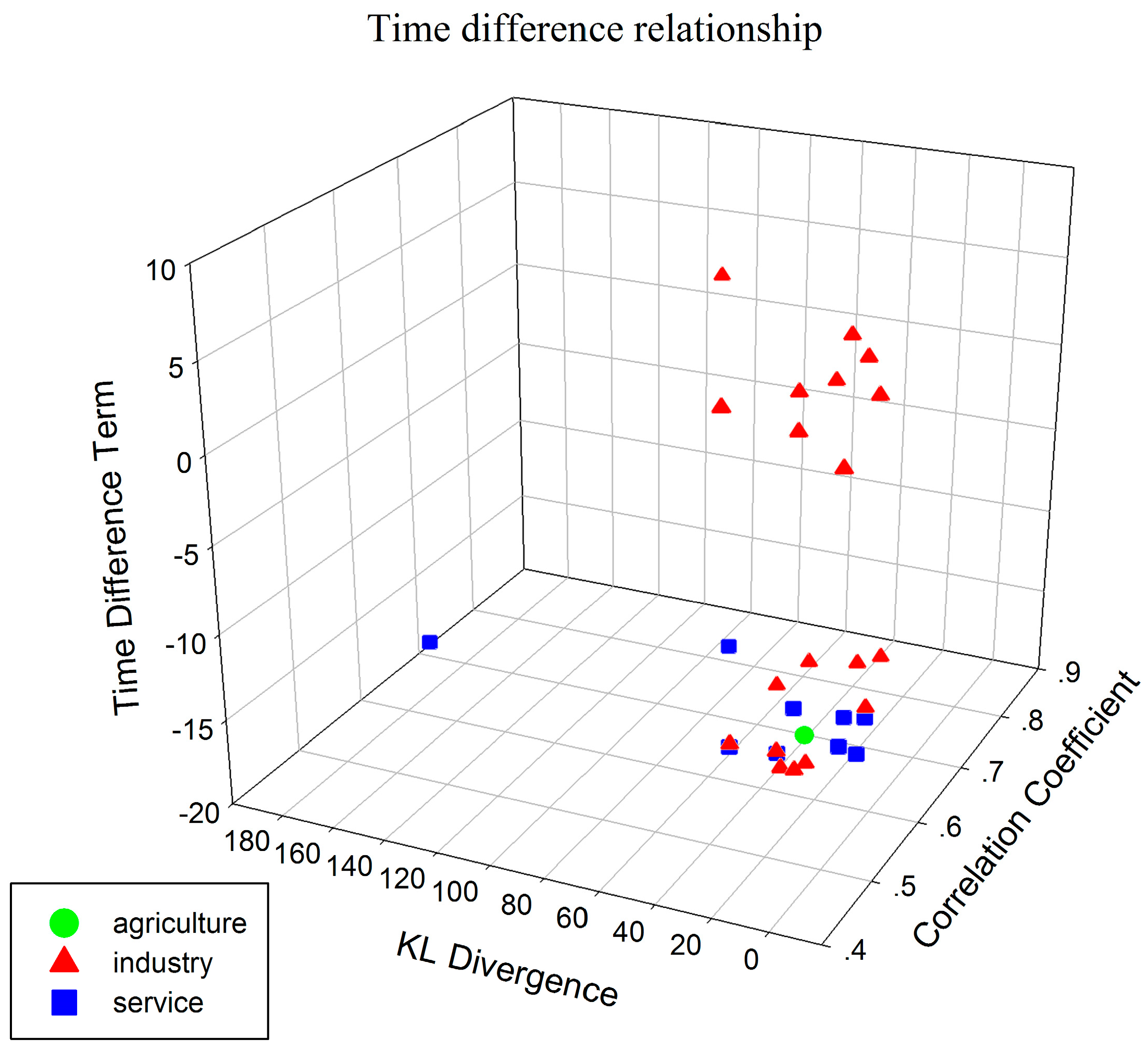
The results of the time difference relationship does not show that the electricity consumption growth of all sectors has an obvious time difference relationship with economic growth. On the basis of the correlation coefficient greater than 0.5, this value is generally considered to indicate a correlation, a total of 29 sectors distributed in various industries can be selected for further analysis on the time difference relationship between sectoral electricity consumption growth and economic growth. There are 20 sectors whose electricity consumption growth has a leading relationship with economic growth, including one sector of agriculture, 10 sectors of industry, and nine sectors of service. All of the seen lagging sectors, and the remaining two synchronous sectors, come from industry. As shown in
Figure 5, the time difference terms of all sectors present a state of aggregation viewed from the time difference term axis in spite of the difference existing in the correlation coefficient and KL divergence. The time difference terms of sectors with a leading characteristic are concentrated around 16 months with the distribution range from 15 months to 18 months. By contrast, the time difference terms of sectors with a lagging characteristic are scattered with a shorter length of time. These time difference terms are distributed within four months of which the longest one is four months from S23. Taking into account two synchronization sectors, the non-negative value of time difference terms vary from 0 to 4.
The time difference relationship between sectoral electricity consumption growth and economic growth varies in different sectors, while there are no obvious rules to follow. According to the results, whether from the sectors selected based on the correlation coefficient or from all sectors, the leading relationship accounted for the majority of all time difference relationships. Additionally, the time difference term of the leading relationship is generally longer than that of the lagging relationship. This shows that different sectors affect the relationship between the total electricity consumption and economic growth to different degrees. Sectors with lagging relationship are mainly from industry and have high electricity consumption, which will have a greater impact on the time difference characteristics of the total electricity consumption. The four major electricity consumption sectors, including manufacture of chemical raw materials and chemical products, manufacture of non-metallic mineral products, smelting and processing of ferrous metals, and smelting and processing of non-ferrous metals, corresponding to sector code S16, S20, S21, and S22, are often mentioned in the analysis of China’s electricity consumption because they account for more than a quarter of the total electricity consumption in China. In 2015, these four sectors consumed 30.24% of the total electricity consumption, of which the sector of smelting and processing of ferrous metals consumed 511.58 TWH, which accounts for 9.22%. In these four sectors, S16 and S22 show the lagging characteristics. In contrast, S20 shows the leading relationship and S21 is synchronized.
The results indicate the time difference relationship between sectoral electricity consumption and economic growth, as well as the asynchronous nature of sectoral electricity consumption. The electricity consumption of different sectors show different degrees of correlation with economic growth. Industry has all three types of sectors with different time difference relationship, while agriculture and service have similar characteristic sectors, most of which show a leading relationship. In a sense, sectors with a leading relationship, a high correlation coefficient, and a small KL divergence can indicate the trend of economic growth in the future for some time through the change of its electricity consumption, while sectors with a lagging relationship, a high correlation coefficient and a small KL divergence can reflect the trend of changes in its electricity consumption associated with economic growth. The time difference relationship between electricity consumption growth and economic growth in these sectors will contribute to the exploration of the economic trends and formulation of relevant policies.


