Operating Energy Savings of a Liquid Desiccant and Evaporative Cooling-Assisted Air-Handling System in Marine Applications

Abstract

The aim of this study is to analyze the operating energy savings of a liquid desiccant and an indirect and direct evaporative cooling-assisted 100% outdoor air system (LD-IDECOAS) for marine applications. The LD-IDECOAS comprises a liquid desiccant (LD) unit and indirect and direct evaporative coolers (IEC and DEC) to meet the target supply air (SA) conditions. In this study, seawater was used as the cooling source and the waste heat reclaimed from the engine was used as the heating source in the proposed system. The operating energy of the LD-IDECOAS was determined based on detailed energy simulations conducted on two cabins with an area of 16.5 m², which was compared to a conventional system. The thermal loads on the cabins were estimated using design weather data under various oceanic climate conditions (normal, extremely hot, and extremely cold climates), by adhering to the ISO-7547 standard. The operating energy consumption of the LD-IDECOAS was calculated by modeling the proposed system with a commercial equation solver program (i.e., EES). The results were then compared to those of a conventional constant air volume (CAV) system. The operating energy consumption of the proposed system was reduced by 57–70% in cooling operations and 39% in heating operations under normal climate conditions. In the extremely hot climate regions, the energy consumed by the proposed system was reduced by 56–63% for cooling applications and 39% for heating applications.

1. Introduction

A liquid desiccant and an indirect and direct evaporative cooling-assisted 100% outdoor air system (LD-IDECOAS) has been proposed as an alternative to conventional heating, ventilation, and air conditioning (HVAC) systems [1,2]. The LD-IDECOAS is a non-vapor compression air-conditioning system based on liquid desiccant (LD) and evaporative cooling technologies [3]. In the LD-IDECOAS, only 100% outdoor air (OA) is used as the supply air (SA), to prevent cross contamination due to mixing with the exhaust air (EA) stream. The supply air flow rate is modulated based on the air conditioning demand inside the conditioned space (similar to a conventional variable air volume (VAV) system).

While processing the outdoor air, the LD-IDECOAS removes the latent heat load from the outdoor air via the LD unit. Subsequently, the sensible cooling load of the outdoor air is accommodated using the indirect evaporative cooler (IEC) and/or the direct evaporative cooler (DEC) [1]. When the outdoor air is dehumidified in the LD unit, the desiccant solution should be cooled before the absorber and heated before the regenerator [4]. The operation modes of the LD-IDECOAS and each system component have been addressed in the literature [2,3].

In marine applications, conventional vapor-compression systems are typically used as air conditioning systems. In ISO-7547 [5], the air conditioning method used in marine spaces was similar to that used in buildings (i.e., conventional constant air volume (CAV) and VAV systems). In addition, the ASHRAE handbook states that HVAC systems proposed for marine spaces are based on the standards for building air conditioning systems [6].

Recently, for building HVAC systems, non-vapor compression systems based on an LD with evaporative cooling systems have attracted significant interest because of their energy and environmental benefits [3,7]. The advantage of the LD system is that its energy consumption can be reduced when operated with evaporative cooling systems [3]. Conventional vapor-compression systems remove the latent heat load of outdoor air via condensation as it passes through cooling coils, by lowering their temperature to the outdoor air dew-point temperature. However, the LD system can directly remove the latent heat load of outdoor air using the liquid desiccant solution. In addition, conventional refrigerants are not employed in non-vapor compression systems, as they deplete the ozone layer, thus avoiding environmental pollution.

In addition to the LD-IDECOAS proposed by Kim et al. [1,2], Kozubal et al. [8] proposed a desiccant-enhanced evaporative air conditioner (DEVap) for air conditioning common buildings. Buker et al. [9] proposed and empirically analyzed a similar air-handling system [1,2,8], which was integrated with a photovoltaic and a thermal roof collector as regeneration heat sources. Gao et al. [10] proposed and evaluated the system performance of a solid-desiccant-enhanced, counter-flow indirect evaporative cooling system. They obtained the optimum process at a specific air temperature and humidity ratio (i.e., 35 °C and 18 g/kg), and demonstrated the performance of the system in humid climates. Ham and Jeong [11] proposed a new type of dew-point evaporative cooler, comprising a dew point evaporative heat exchanger (DPHX) with an LD system.

Only a few applications of non-vapor compression air conditioning systems have been observed in marine spaces. In marine applications, seawater can be used as the water-side free-cooling source [12]. In addition, several studies have focused on the application of reclaiming the waste heat from the engine of a ship, which is a useful heating source for HVAC systems. Aghaali and Angstrom [13] presented a review study on waste-heat recovery systems of internal combustion engines. Shu et al. [14] studied the waste heat released from two-stroke internal combustion engines. Grljusic et al. [15,16] investigated the possibility of combined heat and power (CHP) applications using the waste heat released from the engine of a marine power plant. They performed a thermodynamic analysis of the power plant of a ship operating with waste-heat recovery and estimated the efficiency of the power plant operation. They demonstrated that the waste heat released from the engine could be used in marine HVAC systems. There are also established studies that have proposed empirical models to predict the thermal efficiencies of engine waste heat recovery systems [17,18]. However, only a few studies have considered using engine waste-heat recovery in non-vapor compression air conditioning systems for marine spaces.

Thus, this study evaluated the applicability of an LD-IDECOAS, which is a non-vapor compression air conditioning system, for marine spaces. To estimate the energy performance of the proposed system in air conditioning marine spaces, the thermal load of the model space was initially calculated based on the outdoor air conditions proposed in ISO-7547. Thereafter, the operating energy consumption of the LD-IDECOAS was estimated and compared to that of a conventional CAV system. The outdoor air design conditions for representative climates (i.e., normal, extremely hot, and extremely cold climates) recommended in the ASHRAE handbook [19] were also used to perform the energy simulations in this study. The energy consumptions of the LD-IDECOAS and conventional CAV system under peak thermal loads were evaluated using a commercial equation solver [20].

In this study, to evaluate the applicability of the LD-IDECOAS in marine applications, the LD-IDECOAS characteristics and mode of operation are explained based on the oceanic climate outdoor air conditions. A detailed energy simulation was conducted to estimate the system performance under the design conditions and selected climate zones, which was compared with the operating energy consumption of a conventional CAV system. The energy simulation was performed based on the regional climate zones, which were divided into normal, extremely hot, and extremely cold, respectively.

2. Liquid Desiccant and Evaporative Cooling-Assisted Air-Handling System

2.1. System Overview

This section is divided into subsections, to provide a concise and precise description of the experimental results, their interpretation, and the experimental conclusions that can be drawn. The LD-IDECOAS uses 100% outdoor air as the supply air for the conditioned space, and it can be divided into two main parts (Figure 1). Upstream of the process air, an LD unit is installed for the dehumidification of the outdoor air. Downstream of the LD unit, an IEC and a DEC are installed for sensible cooling of the process air, to meet the target supply air condition. The induced outdoor air is dehumidified using the LD system, and sensible cooling is performed by continuously passing the air through the IEC and DEC. To achieve a high sensible cooling effect in the IEC, exhaust air can be fed into the secondary channel of the IEC when the wet-bulb temperature (WBT) of the exhaust air is lower than that of the outdoor air. A sensible heat exchanger (SHE) and a heating coil (HC) are located in the exhaust air duct to maintain the exhaust air conditions necessary to use it as a secondary air source in the IEC. The supply air flow rate is adjusted based on the cooling load required for the conditioning room, which is similar to the working of a conventional VAV system.

The operation modes of the LD-IDECOAS are determined based on the outdoor air conditions, which are categorized into four regions (Figure 2) on the psychrometric chart [2]. In region A, the outdoor air is hot and humid. To meet the supply air target condition, the introduced outdoor air is initially dehumidified using the LD; subsequently, the process air undergoes sensible cooling in the IEC and adiabatic cooling in the DEC. When the outdoor air condition is located in region B or region C, the LD-IDECOAS meets the supply air conditions by only operating the IEC and/or DEC, without LD operation. In region D, the IEC operates as a SHE, without injecting water into the secondary channel of the IEC. The waste heat from the exhaust air is recovered using the IEC, to reduce the sensible heating load of the outdoor air. Moreover, additional heat recovery is possible using the SHE (installed at the terminal box).

2.2. Operation Modes of LD-IDECOAS

The outdoor air in region A is hot and humid [2]. To meet the target temperature of the supply air, the LD-IDECOAS should be operated at its full capacity. As shown in Figure 1, initially, the moisture from the outdoor air is removed using the LD system, until the humidity ratio represented by the line “a” on the psychrometric chart is obtained. After the dehumidification process, the process air is adjusted to the supply air set-point temperature (i.e., 15 °C), by sequentially passing it through the IEC and DEC. The process air entering the IEC is sensibly cooled, and subsequently, adiabatically cooled in the DEC. Before the supply air is supplied to the room, the supply air should reach a target temperature of 15 °C; moreover, the supply air should be saturated (Figure 3).

In regions B and C, the LD-IDECOAS is operated based on the sensible cooling of the outdoor air; hence, the LD system is deactivated. The induced outdoor air bypasses the LD and sensibly cools in the IEC, to meet the supply air target temperature. The DEC is operated to provide adiabatic cooling in order to meet the supply air condition. The boundary between the regions B and C is defined by the outdoor air enthalpy line. If the enthalpy of the outdoor air is lower than that of the target supply air condition (i.e., 15 °C or 42.1 kJ/kg), the condition corresponds to region C, for which the target supply air temperature can be met by only operating the DEC (Figure 4).

Finally, in region D (Figure 5), when the dry-bulb temperature (DBT) of the outdoor air is lower than the target supply air temperature, the LD unit and DEC remain switched off. Additionally, the IEC operates as a SHE, without spraying water into the secondary channel of the IEC. The waste-heat energy recovered from the exhaust air stream is used in the IEC. If the supply air temperature is not sufficiently high to meet the target temperature (i.e., the neutral temperature of the air-conditioned space), the HC is operated to add sensible heat to the heat recovered from the exhaust air stream.

Table 1. Operation modes of the LD-IDECOAS.

Region	LD	IEC	DEC
A	On	On	On
B	Off	On	On
C	Off	Off	On
D	Off	On (dry mode)	Off

lists the operation modes of the LD-IDECOAS corresponding to the various outdoor air conditions.

3. Research Methodology

To analyze the applicability of the LD-IDECOAS as an HVAC system for air conditioning marine spaces, the operating energy consumption was compared with that of a conventional system (Figure 6). The operating energy consumptions of the proposed and conventional systems were estimated by performing detailed energy simulations based on the air conditioning demands of the model space. The thermal demands of the model space were determined based on the design outdoor air conditions provided in ISO-7547 [5] and the representative climate zones (i.e., normal, extremely hot, and extremely cold climates) recommended in the ASHRAE handbook [19].

3.1. Outdoor Air Design Condition

The peak thermal loads of the model space were estimated using the calculation method recommended by ISO-7547, which utilizes the load calculation procedure and basic assumptions that are critical for designing HVAC systems serving passenger cabins in ships [5]. In ISO-7547, the outdoor air condition with a 35 °C dry bulb and 70% relative humidity was suggested for the summer design condition, and a −20 °C dry bulb was provided for the winter design condition. The design room air conditions used a 27 °C dry bulb and 50% relative humidity for the summer and a 22 °C dry bulb for the winter. ISO-7547 does not specify the design humidity level for the outdoor air and the room air for winter operation. The design conditions provided in ISO 7547 should only be used in normal climate regions and not in extremely cold or hot climates. Hence, to estimate the thermal load of the design space under various climate conditions, the ASHRAE design weather conditions [19] were employed for seven selected climate regions (i.e., three normal climate regions, two extremely hot climate regions, and two extremely cold climate regions) (Figure 7). Accordingly, the simulations of both the LD-IDECOAS and the conventional CAV system were performed.

The outdoor air design conditions for each selected region are specified using the DBT and humidity ratio, which have a cumulative occurrence frequency of 0.4% or 1%. The design condition with a cumulative occurrence frequency of 0.4% was selected to estimate the regional peak thermal loads of marine spaces.

Table 2. OA design conditions of selected climate zones.

Climate	Region	Cooling Design Conditions	Heating Design Conditions	Location
Normal climate	Horta (Atlantic)	25.8 °C, 72.3%	9.8 °C	38.5° N, 28.7° W
	Plaisance (Indian Ocean)	30.8 °C, 66.8%	16.2 °C	20.4° N, 57.7° E
	La Roche (Pacific Ocean)	30.1 °C, 67%	9.2 °C	21.5° S, 168.0° E
Extremely hot climate	Hawaii (Pacific Ocean)	27.9 °C, 60%	-	13.5° N, 144.8° E
	Virgin Islands (Atlantic)	32 °C, 60.3%	-	17.7° N, 64.8° W
Extremely cold climate	Halley (Antarctic)	-	−45.8 °C	75.5° S, 26.7° W
	Polargmo (Arctic)	-	−37.3 °C	80.6° N, 58.1° E

lists the regional outdoor air design conditions used in this study.

3.2. Thermal-Load Calculation

Based on ISO-7547, the transmission heat losses and gains for each marine space surface can be calculated using Equation (1). To estimate the heat transmission through the external deck and window, the total heat transfer coefficients of the external deck and window were assumed to be 0.9 and 3.5 kW/m²K, respectively. The heat transmission between the cabins was neglected based on the assumption that the indoor air temperature in each cabin (i.e., 27 °C) was identical.

Table 3. Geometry and physical information of the deck and window [5].

Deck	Window
Type: plane insulation of uniform thickness	Type: round side scuttles of 2.26 m2
Total heat-transfer coefficient: 0.9 kW/m2 K	Total heat-transfer coefficient: 3.5 kW/m2 K

lists the geometry and physical information of the deck and window of each cabin.

$$Q=\mathit{\Delta }T\times \left[\left(K_v\times A_v\right)+\left(K_g\times A_g\right)\right]$$

(1)

where $K_v$ is the heat transfer coefficient of the external surface in (W/(m² °C)) and $K_g$ is the heat transfer coefficient of the external glass window in [W/(m² °C)].

The solar heat gain from the external surfaces exposed to solar radiation was calculated using Equation (2), as recommended in ISO-7547. For the external deck, the direction and color are important factors in determining the solar heat gain. In this study, the solar heat gain of the external deck was calculated by assuming a horizontal, light-colored surface (i.e., $\mathit{\Delta }{T}_r$ in Equation (2) is 15 °C). The solar heat gain from the window was estimated by employing the solar heat gain factor suggested in ISO-7547. The solar heat gain factor of the clear glass window scuttles without interior shading was 350 W/m².

$$Q_s=\Sigma A_{v}K\mathit{\Delta }{T}_r+\Sigma A_g{G}_s$$

(2)

where $K$ is the total heat transfer coefficient of the external surface in (W/(m² °C)), $\mathit{\Delta }{T}_r$ is the temperature difference between the external and internal surface at 15 °C, and $G_s$ is the solar heat gain factor of the clear glass window scuttles in (W/m²).

The sensible and latent heat gains from a person exerting medium work were assumed to be 70 W/person and 50 W/person, respectively. If a person is doing heavy work, a sensible heat of 85 W/person and latent heat of 150 W/person can be assumed. For the lighting heat gain, fluorescent lighting equipment was assumed; the lighting equipment yielded a sensible heat emission of 8 W/m². The maximum occupant density suggested in ISO-7547 for the accommodation spaces and passenger cabins (i.e., 3 persons/m²) was considered in this study. Because of the high level of air-tightness in ship spaces and the design proposal given in ASHRAE handbook, air infiltration and leakage in the cabin were neglected while calculating the thermal load [6].

Table 4. Physical parameters of the model space for calculating the thermal load.

Number of Spaces	2
Schedule	On board: for one hour
Room conditions	Summer: 27 °C, 50%, Winter: 22 °C
Cabin area	33 m2 (16.5 m2 each)
Window-to-deck ratio	15%
Occupants	People: 10 (Sensible heat: 70 W/person; latent heat: 50 W/person)
Lighting	8 W/m2 (fluorescent lighting)

lists the physical information of the modeled cabin spaces.

Additionally, because a ship continuously sails on the sea and cannot be considered a building, the hourly energy simulation approach typically applied to buildings cannot be employed; thus, the energy performances of both the proposed and conventional CAV systems were compared to obtain the peak thermal loads.

3.3. Energy Simulation

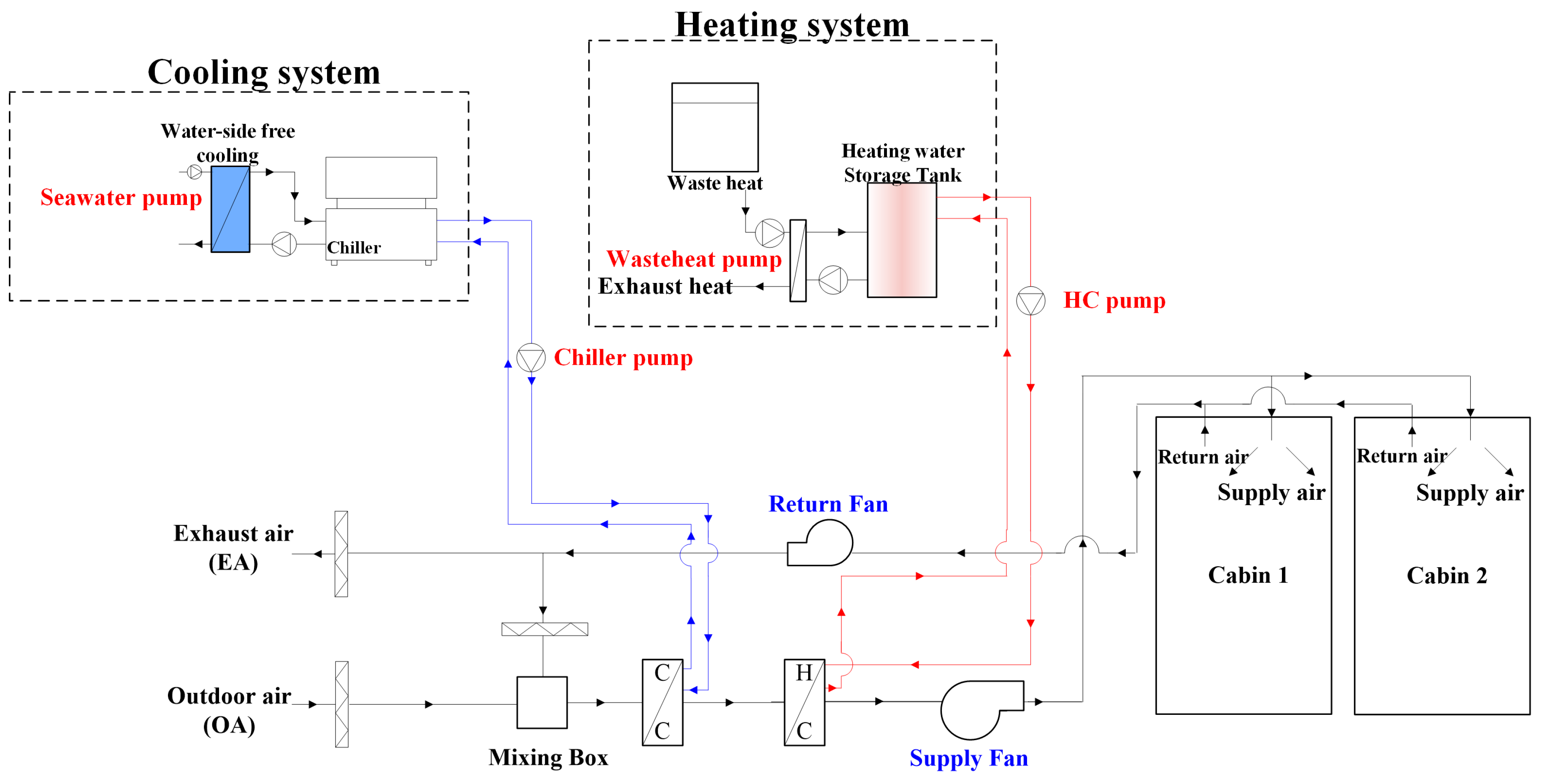
3.3.1. Constant Air Volume System

Figure 6 shows the configuration of the conventional CAV system considered in this study. The energy consumption of the CAV system was calculated based on the predicted peak thermal loads of the model space. Based on ISO-7547, the cooling set-point of the conditioned space was 27 °C with 50% relative humidity, and the heating set-point was 22 °C, without considering humidity control. In the cooling operation, the supply air was cooled, and subsequently dehumidified using the cooling coil. The supply air flow rate was maintained at 1200 m³/h, wherein 40% of the supply air flow (i.e., 480 m³/h) comprised fresh outdoor air introduced for ventilation (in accordance with ISO-7547). The conventional CAV system was able to meet the thermal load by means of supply air temperature control, while the design supply air temperature was 13 °C. A DOE-2 air-cooled chiller model with a coefficient of performance (COP) of 2.95 was applied in this simulation [21,22]. The energy of the chiller was calculated using Equation (3), considering the part load ratio of the chiller. The power demand of the reference chiller was estimated using Equation (4), based on the reference chiller capacity and COP.

$$\mathrm{P}={\mathrm{P}}_{ref}\times PTR$$

(3)

where ${\mathrm{P}}_{ref}$ is the reference chiller power in (W).

$${\mathrm{P}}_{ref}={\dot{Q}}_{ref}\times CO{P}_{ref}$$

(4)

where ${\dot{Q}}_{ref}$ is the reference chiller capacity in (kW).

Alternatively, the water-side free cooling with seawater was considered during the chiller operation to reduce the energy consumption of the chiller. The temperature of seawater in the summer was assumed to be 20 °C, based on the literature [23]. The efficiency of the SHE was set to 70%. To estimate the energy consumption of the seawater pump using Equation (5), the pump was assumed to be a constant-flow pump with an efficiency of 60% and a head of 20 m [22].

$${\mathrm{P}}_{design,pump}=\frac{V\times H\times 10}{{\eta }_{pump}}$$

(5)

where $V$ is the volume flow rate in (m³/s), $H$ is the pump head in (m), and $\eta$ is the pump efficiency in (-).

The HC was activated as a reheating coil to meet the supply air conditions and adjust the thermal load of the conditioning space. During operation in the winter season, the HC was operated to maintain the heating temperature set-point of the supply air (i.e., 45 °C), with a design supply air flow rate of 400 m³/h. The intake flow rate of the outdoor air for ventilation was 160 m³/h (i.e., 40% of the supply air flow rate).

3.3.2. LD-IDECOAS

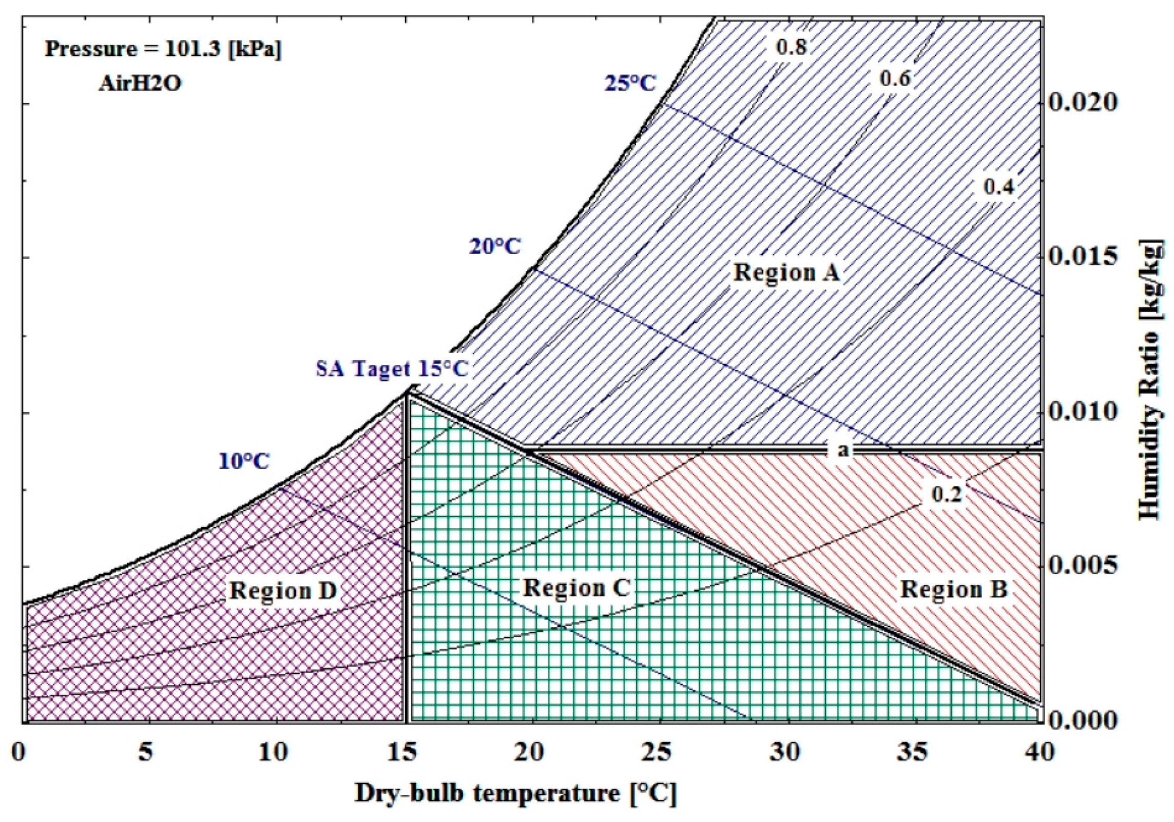
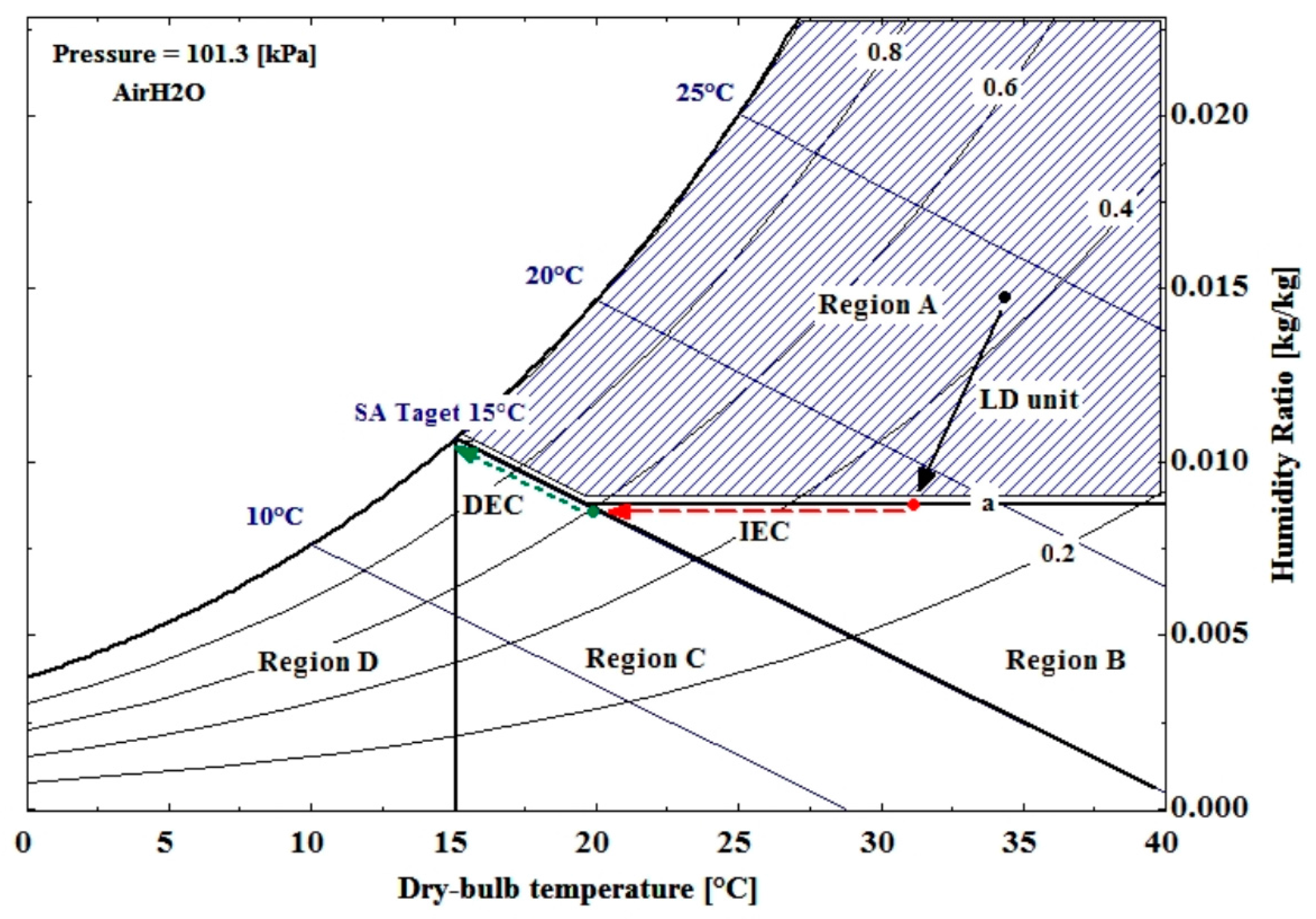
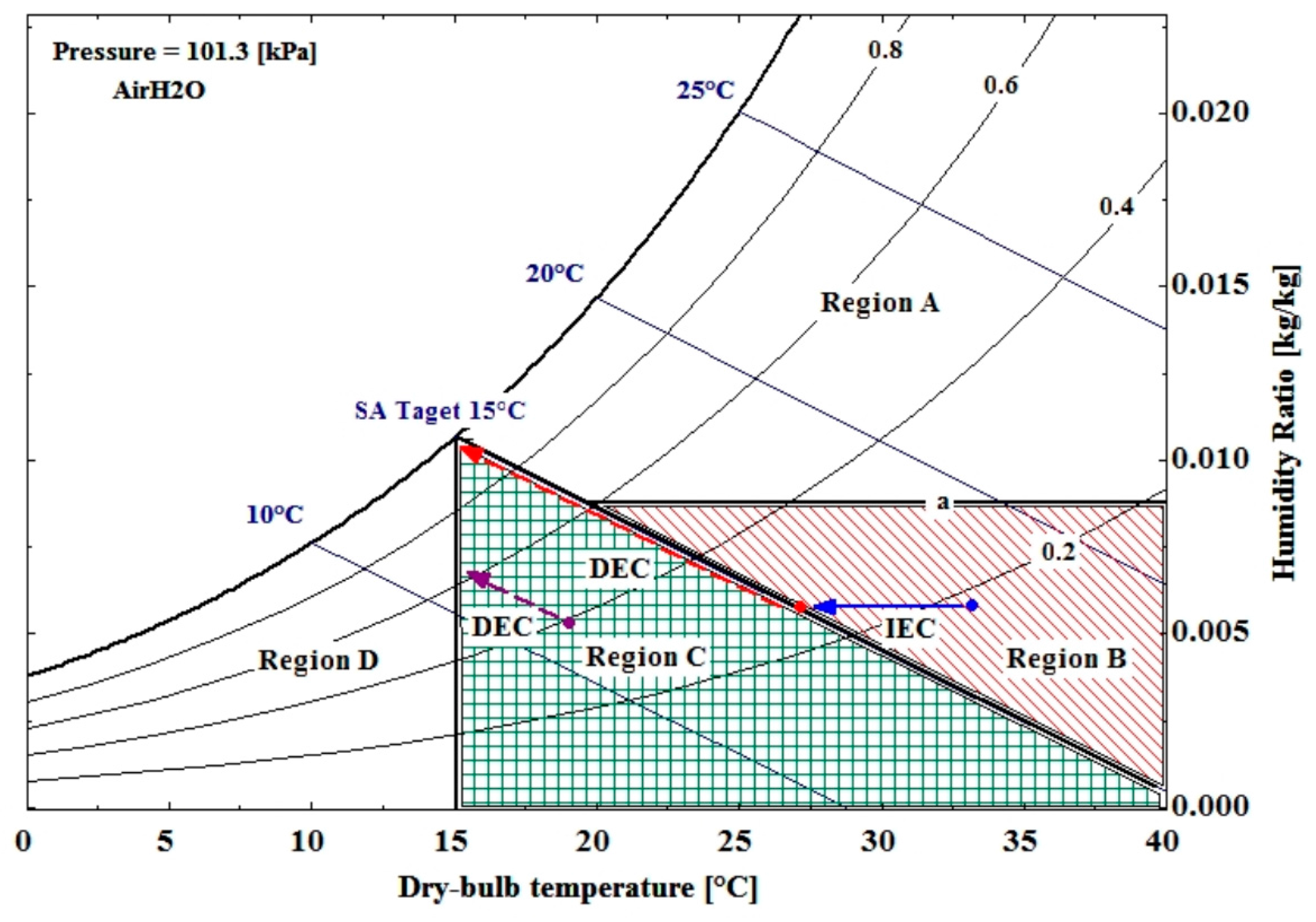
Considering the energy consumption of the LD-IDECOAS in summer conditions, the outdoor air is in region A on the psychrometric chart (Figure 2). Thus, the equipment present within the LD-IDECOAS should be operated. To meet the supply air condition (i.e., 15 °C), the induced outdoor air is dehumidified using the LD, before entering the IEC. After dehumidification, the process air enters the IEC for sensible cooling, and subsequently enters the DEC for adiabatic cooling, to meet the supply air conditions. The outdoor air conditions in winter correspond to region D on the psychrometric chart. For outdoor air conditions within this region, the LD system of the LD-IDECOAS is bypassed. The heat recovered from the exhaust air stream preheats the induced outdoor air in the IEC. The IEC operates in a similar manner to a SHE, without spraying water into the secondary channel of the IEC. When the supply temperature is not sufficiently high to meet the supply air conditions after IEC and SHE operations, the HC is operated to ensure the high sensible heat of the supply air condition (i.e., 45 °C).

The process air condition at the outlet of the LD unit ($T_{LD}$) was determined using Equation (6), whereas the outdoor air temperature ($T_{oa}$), inlet temperature of the solution ($T_{si}$), and temperature efficiency were known values (${\epsilon }_{LD,T}$). In addition, the DBT condition of the process air at the outlet of the IEC ($T_{IEC}$) was calculated using Equation (7), as the efficiency of the IEC (${\epsilon }_{IEC}$) was known. In this study, the efficiency of the IEC was assumed to be 70% [24]. Moreover, the inlet WBT condition of the secondary air ($WB{T}_{sec,IEC}$) was considered the same as that of the WBT condition of the exhaust air (Figure 1). Similarly, the DBT condition at the outlet of the DEC ($T_{DEC}$) was the target DBT condition of the supply air ($T_{sa}$), which was estimated using Equation (8) for a given efficiency of the DEC (${\epsilon }_{DEC}$); herein, the efficiency of the DEC was assumed to be 95% [24]. The humidity ratio of the outlet condition of the LD unit (${\omega }_{LD}$) was determined using Equation (9), for an assumed dehumidification efficiency of the LD unit (${\epsilon }_{LD,\omega }$). Based on the literature, the temperature efficiency of the LD unit (${\epsilon }_{LD,T}$) was found to be similar to its dehumidification efficiency (${\epsilon }_{LD,\omega }$) [25,26].

$${\epsilon }_{LD,T}=\frac{\left(T_{oa}-T_{LD}\right)}{\left(T_{oa}-T_{si}\right)}$$

(6)

$${\epsilon }_{IEC}=\frac{\left(T_{LD}-T_{IEC}\right)}{\left(T_{LD}-WB{T}_{sec,IEC}\right)}$$

(7)

$${\epsilon }_{DEC}=\frac{\left(T_{IEC}-T_{DEC}\right)}{\left(T_{IEC}-WB{T}_{IEC}\right)}$$

(8)

$${\epsilon }_{LD,\omega }=\frac{\left({\omega }_{oa}-{\omega }_{LD}\right)}{\left({\omega }_{oa}-{\omega }_e\right)}$$

(9)

The dehumidification effectiveness of the LD was evaluated using an existing model (Equations (10) and (11)) found in the literature [27,28]. The model is an empirical model applicable to an LD unit with a lithium chloride (LiCl) solution. In addition, the regeneration effectiveness of the LD unit was determined using Equations (12)–(14), by employing the coefficients listed in

Table 5. Coefficients of the regeneration effectiveness model [29].

C1	b	${\mathit{\gamma }}_{\mathit{t}}$	${\mathit{k}}_{\mathbf{1}}$	${\mathit{m}}_{\mathbf{1}}$	${\mathit{k}}_{\mathbf{2}}$	${\mathit{m}}_{\mathbf{2}}$
48.3	−0.751	61	0.396	−1.57	0.0331	−0.906

[29]. The thermodynamic characteristics of the LiCl solution were obtained from the literature [20,30].

$${\epsilon }_{LD}=\frac{[1-(0.024{({\mathsf{ṁ}}_{ai}/{\mathsf{ṁ}}_{si})}^{0.6}\exp (1.057(T_{oa}/T_{si})))/({\left(a{Z}_t\right)}^{-0.185}{\pi }^{0.638})]}{\left[1-\left(0.192\exp \left(0.615\left(T_{oa}/T_{si}\right)\right)\right)/\left({\pi }^{-21.498}\right)\right]}$$

(10)

where:

$$\pi =\left(P_{wa\left(T_{si}\right)}\right)-(P_{so\left(T_{si},X_{si}\right)})/\left(P_{wa\left(T_{si}\right)}\right)$$

(11)

$${\epsilon }_{Reg}=1-C_1{\left(L/G\right)}^a{\left(H_{ai}/H_{si}\right)}^b{\left(a{Z}_t\right)}^c$$

(12)

where:

$$a=k_1\left({\gamma }_{si}/{\gamma }_t\right)+m_1$$

(13)

$$c=k_2\left({\gamma }_{si}/{\gamma }_t\right)+m_2$$

(14)

To evaluate the system performance of the LD unit, the operating conditions of the system were adjusted using the initial conditions. The LD unit was modeled with the LiCl solution as the desiccant material. An inlet temperature of 30 °C (obtained by adjusting the seawater free cooling) and an inlet concentration of 40% were considered for the solution. The thermal load of the regeneration energy of the desiccant solution was considered, depending on the moisture removal rate. The weak desiccant solution must be heated to the regeneration temperature (60 °C) before entering the regenerator.

Alternatively, to estimate the fan energy consumptions of the proposed system, the air-side pressure drop in each system component was considered.

Table 6. Air-side pressure drops for fans.

	Component	Design Pressure ΔP	Specification
LD-IDECOAS	SA fan	805 Pa	Absorber 145 Pa [31], IEC 140 Pa [24], DEC 20 Pa [32], balance of system 500 Pa
	EA fan (IEC)	470 Pa	IEC 220 Pa [24], balance of system 250 Pa
	Regenerator	145 Pa	Design air flow 1200 m3/h
CAV system	SA fan	750 Pa	with balance of system and AHU [22]
	EA fan	200 Pa	with EA duct and plenum [22]

presents the static pressure drops of each component under a design flow rate of 1200 m³/h [22,24,31,32]. The fan energy consumptions were estimated using Equations (15) and (16) for constant and variable flow fans, respectively.

$${\mathrm{P}}_{design,fan}=\frac{\mathsf{ṁ}\times \Delta P}{{\rho }_{ai}\times {\eta }_{fan}}$$

(15)

where $\rho$ is the density of air in (kg/m³) and $\eta$ is the fan efficiency in (-).

$${\mathrm{P}}_{variable}={\mathrm{P}}_{design}{\left(\frac{V_{variable}}{V_{design}}\right)}^3$$

(16)

where $V$ is the volume flow rate in (m³/s).

To estimate the energy consumption of the pump in the proposed system, the head of each pump was determined based on the design flow rate of each pump required in the proposed system. The pump energy consumptions were estimated using Equations (5) and (16) for constant and variable flow pumps, respectively. The efficiency of each pump was assumed to be 60%.

Table 7. Head of each pump.

	Component	Design Pump Head	Specification
LD-IDECOAS	Abs. and Reg. pumps	15 m at 0.33 m3/s	Solution-circulation pump [33]
	IEC and DEC pumps	10 m at 0.001 m3/s	Water-circulation pump [33]
	HC pump	20 m at 0.0011 m3/s	Energy plus model [22]
	Waste-heat pump
	Seawater pump
CAV system	Chiller pump	18 m at 0.28 m3/s	Energy plus model [22]
	HC pump	20 m at 0.0011 m3/s
	Water-heat pump
	Seawater pump

presents the head of each pump considered in this study.

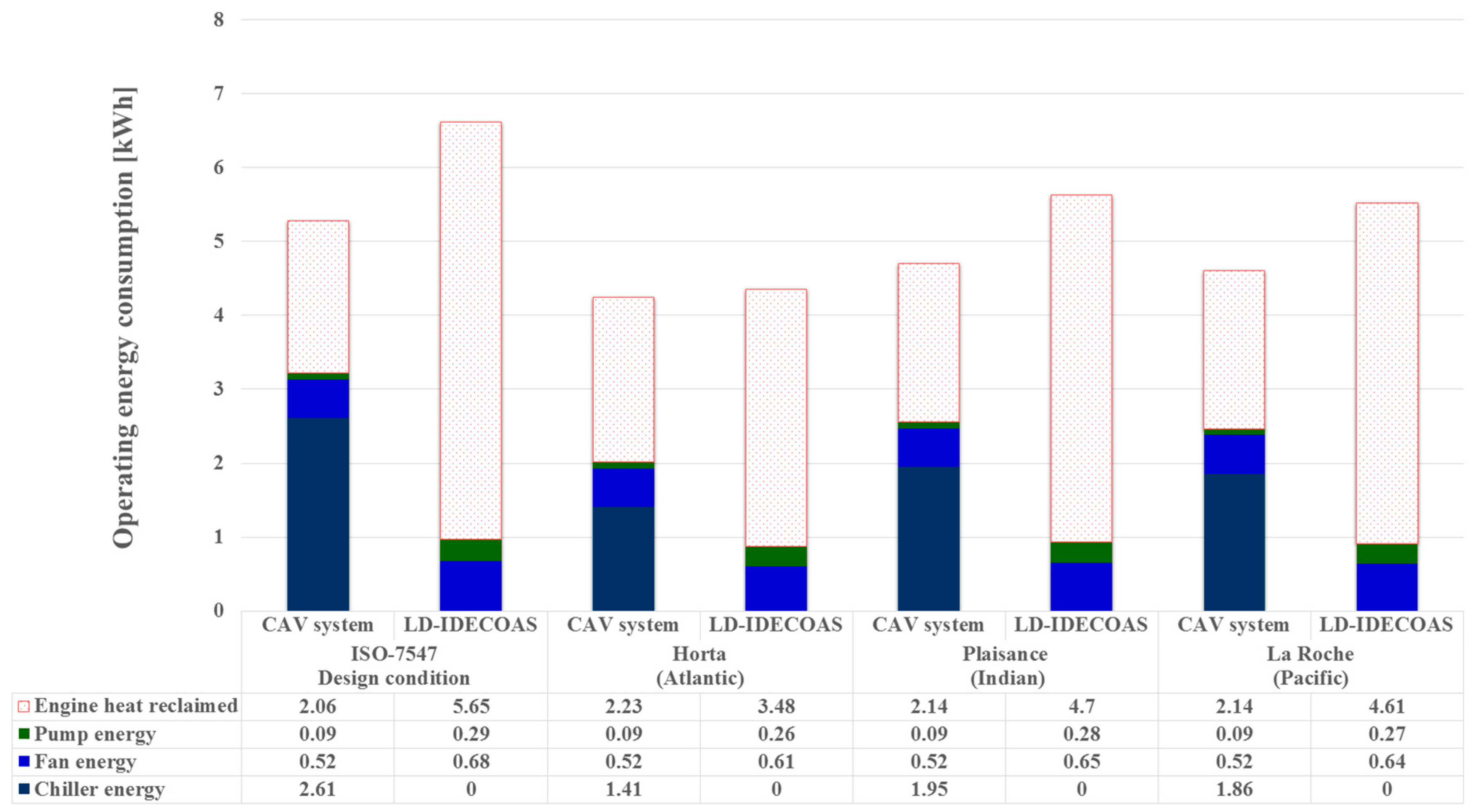
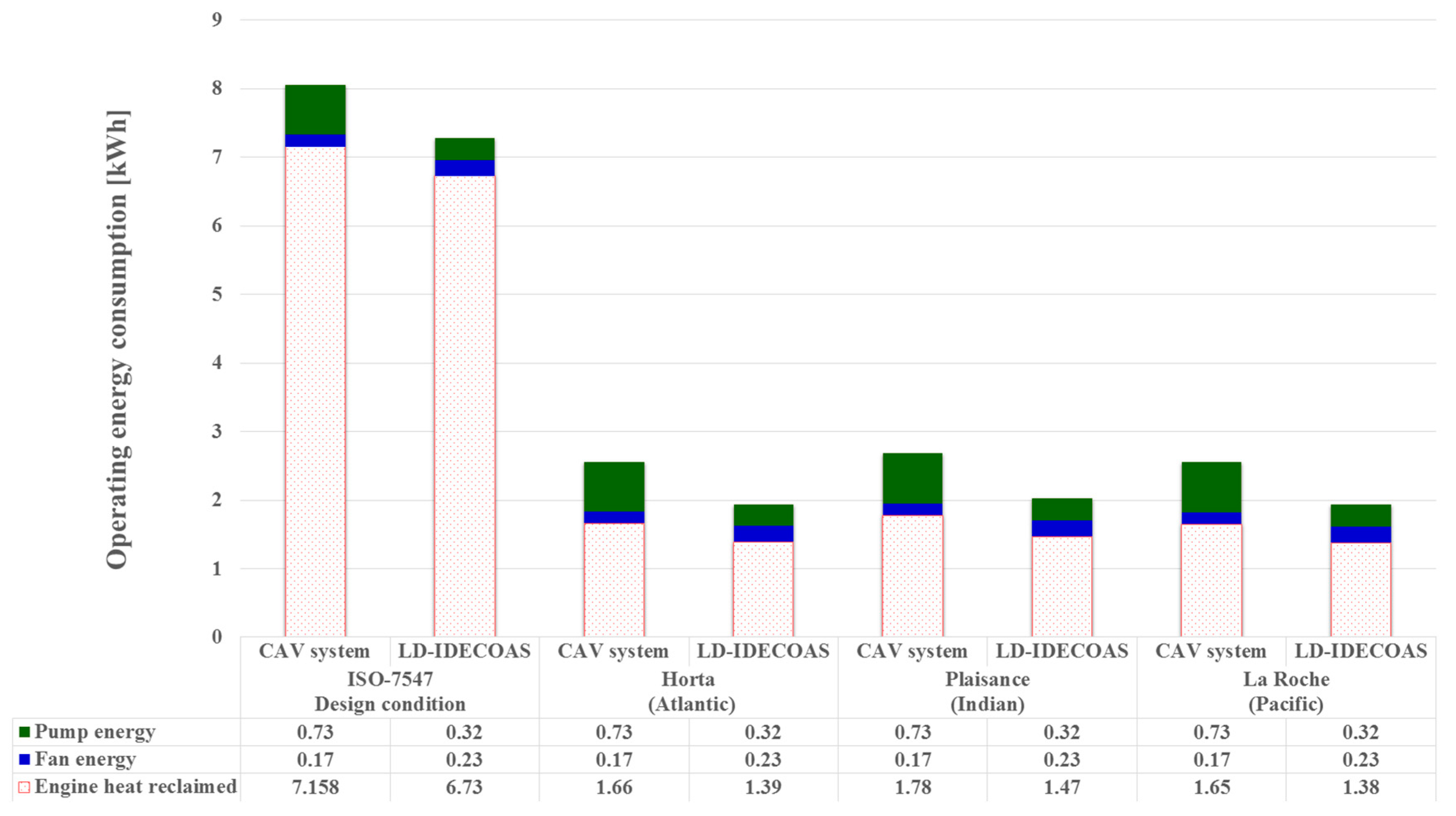
During the operation of the LD unit, a regeneration heat source should be supplied to meet the required solution heating load. In this study, the engine waste heat was considered to be the heat source for regenerating the desiccant solution. Generally, the Rankine cycle is employed for the application of waste-heat recovery to understand the thermal characteristics based on the theory of thermodynamics. The organic Rankine cycle is a promising technology, wherein the waste heat can be used as a renewable heat source without CO₂ emissions. In the present simulation, a prediction model for organic Rankine-cycle heat recovery was used to estimate the quantity of waste heat [15,16,17,18]. 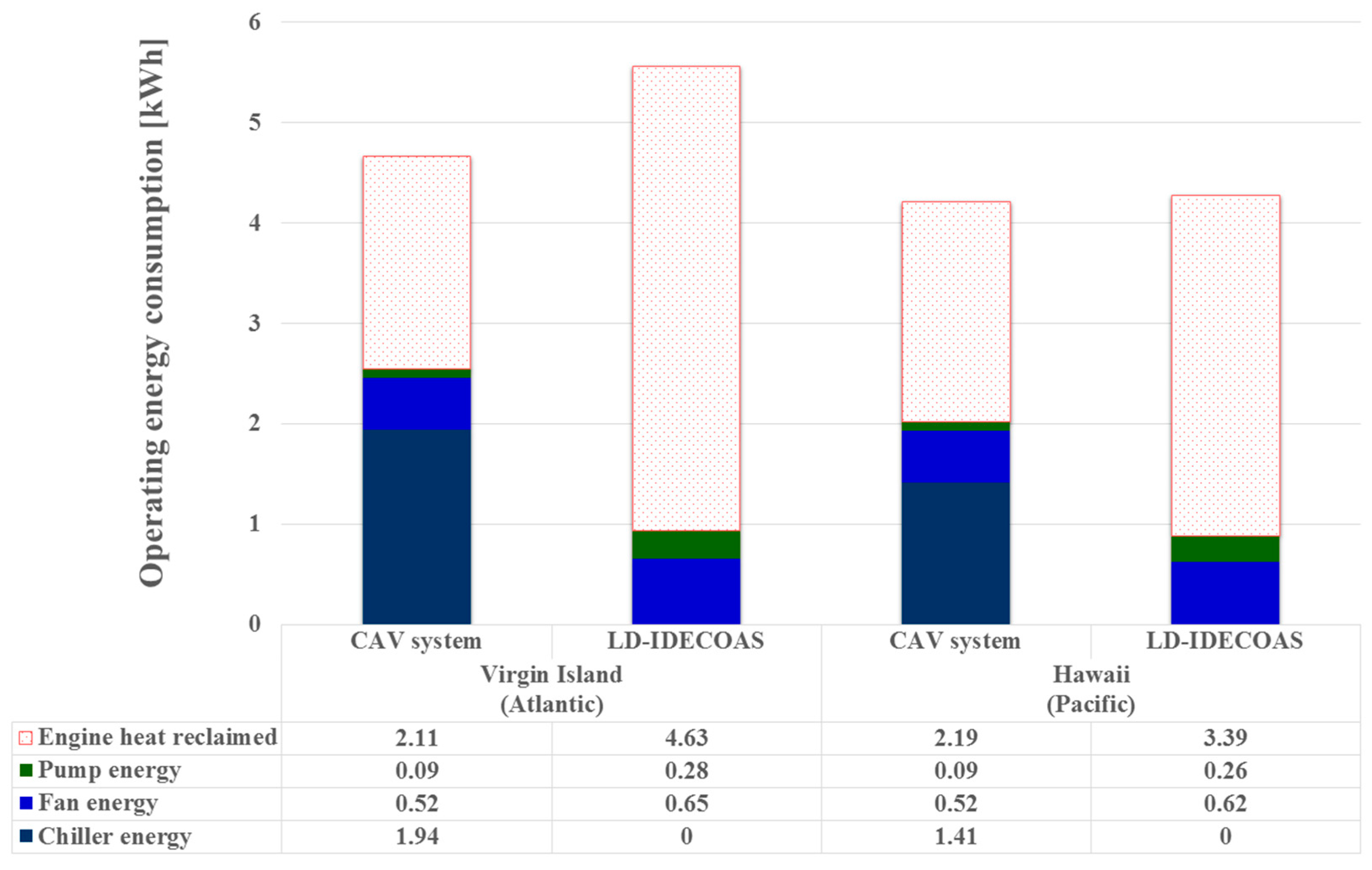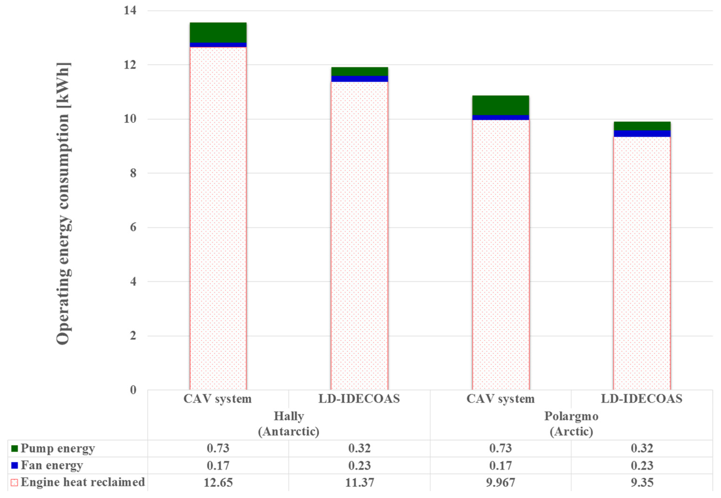To estimate the waste-heat recovery, the efficiency of the organic Rankine cycle was assumed to be 10% and 70% of the efficiency of the waste-heat recovery [18]. Based on this estimation, engine waste heat can be reclaimed at 80 kW/h. Consequently, both of the considered HVAC systems (i.e., the LD-IDECOAS and CAV system) would be able to meet the required system heating load.

4. Simulation Results

4.1. Peak Thermal Loads

The peak cooling and heating loads of the model space were initially estimated based on the design outdoor air conditions and the load calculation procedure proposed in ISO-7547. However, the design outdoor air conditions suggested by ISO-7547 could not accommodate extremely hot or cold climates. Consequently, the ASHRAE design outdoor air conditions [19] for seven representative locations, including extreme climate zones, were considered to estimate the peak cooling and heating loads of the model space. Figure 8 shows the peak thermal loads of the model space estimated for each design outdoor air condition. The results show that the peak thermal loads estimated under the ISO-7547 design outdoor air conditions were 4.59 and 0.86 kW for the cooling and heating loads, respectively. The peak cooling loads in both the normal and extremely hot climate regions were lower than those estimated under the ISO-7547 design outdoor air conditions. However, the peak heating loads estimated for the extremely cold climate regions were higher than those under the ISO-7547 design outdoor air conditions. Alternatively, as listed in Table 2, outdoor air design conditions were not recommended for the heating load calculation in the extremely hot climate regions or cooling load calculation in the extremely cold climate regions. Consequently, as shown in Figure 8, the peak heating loads in the extremely hot climate regions and peak cooling loads in the extremely cold climate regions were zero.

4.2. Energy Consumption in Normal Climates

Figure 9 presents a comparison of the operating energy consumptions of both systems under the peak cooling load conditions estimated for the design outdoor air conditions, as recommended in ISO-7547, as well as those of three representative regions with normal climates in the Atlantic, Indian, and Pacific Oceans. The results show that the energy consumptions of the fan and pump in the LD-IDECOAS were higher than those in the conventional CAV system under each design outdoor air condition. This is because of the additional fans and pumps in the proposed system, which were not required in the conventional system. However, the increased energy consumptions of the pump and fan in the LD-IDECOAS were compensated for by the decreased operational demands of the chiller; the chiller of the CAV system consumed a significant amount of energy.

Alternatively, as shown in Figure 9, the heating energy required for regenerating the desiccant solution in the LD-IDECOAS was higher than the reheating energy in the conventional CAV system. However, the heat for both systems was obtained from a free heat source; the heat was reclaimed from the engine of the ship [15,16,17,18]. Consequently, the operating energy consumptions of both of the systems under the peak cooling load conditions were compared to consider the operating energy consumptions, except for the heating energy.

The results show that the energy consumption of the LD-IDECOAS was 70% lower than that of the CAV system under the peak cooling load estimated for the ISO-7547 design condition. Similarly, the energy consumption of the proposed system was 57% lower at Horta in the Atlantic Ocean, 63% lower at Plaisance in the Indian Ocean, and 63% lower at La Roche in the Pacific Ocean.

Figure 10 shows the comparison of the operating energy consumptions of both the LD-IDECOAS and CAV system under the heating design outdoor air conditions recommended in ISO-7547, as well as under the three representative regions with normal climates in the Atlantic, Indian, and Pacific Oceans (selected from the ASHRAE handbook). The results show that the heating energy required for both of the systems to meet the peak heating demand of the conditioned spaces was significant. Nevertheless, the LD-IDECOAS consumed less heating energy than the CAV, because of the sensible heat recovered from the exhaust air stream via the SHE and IEC during the operation. Moreover, the LD-IDECOAS consumed more fan energy than the CAV system because of the larger air-side pressure drops in the IEC and SHE. However, the increased fan energy consumption was compensated for by the reduced pump and heating energy consumptions.

In marine applications, the heating energy required for both the LD-IDECOAS and CAV system could be supplied by the waste heat reclaimed from the engine [15,16,17,18], which is a free heat source. The heating energy consumptions of both of the systems were compared by considering the operating energy consumptions, except for the heating energy. Thus, this result represents the operating energy consumption during the heating season, considering the energy consumptions of the fans and pumps of both the LD-IDECOAS and CAV system. The results show that the operating energy consumption of the LD-IDECOAS was 39% lower than that of the CAV system under the peak heating load estimated for the ISO-7547 design condition. The reduction in the operating energy of the proposed system was similar under the peak heating loads estimated for the other normal climate regions.

4.3. Energy Consumption in Extremely Hot Climate Zones

Figure 11 shows a comparison of the operating energy consumptions of both the LD-IDECOAS and CAV system estimated under the peak cooling loads in two extremely hot oceanic climate regions: the Virgin Islands in the Atlantic Ocean and Hawaii in the Pacific Ocean. As expected, the proposed system showed higher heating energy demands than the conventional CAV system, because the desiccant solution was regenerated. However, the heating energy demands of both of the systems were met by reclaiming the heat from the engine of the ship; therefore, the use of more reclaimed heat in the proposed system was not a significant disadvantage in terms of energy consumption. Moreover, the LD-IDECOAS showed more fan and pump energy consumptions than the CAV system. However, this disadvantage in the proposed system was compensated for by the decreased energy consumption of the chiller. The operating energy consumptions of both of the systems under the peak cooling load conditions were compared by considering the operating energy consumptions, except for the heating energy. The results show that in the Virgin Islands, the operating energy consumption of the LD-IDECOAS was 63% lower than that of the conventional CAV system. Similarly, the operating energy consumption of the proposed system decreased by 56% in Hawaii.

4.4. Energy Consumption in Extremely Cold Climate Zones

Figure 12 presents a comparison of the operating energy consumptions of both the LD-IDECOAS and CAV system under the peak heating loads in two extremely cold oceanic climate regions: Hally in the Antarctic Ocean and Polargmo in the Arctic Ocean. The results show that the proposed system consumed more fan energy than the CAV system. However, this disadvantage was compensated for by the reduced pumping energy. Although the LD-IDECOAS consumed less heating energy than the CAV system because of the sensible heat recovered from the exhaust air via the SHE and IEC, the heat used in both of the systems was obtained from the reclaimed engine heat, which was neglected in the operating energy comparison. The LD-IDECOAS showed a 39% lower operating energy consumption than the CAV system under peak heating loads in both extremely cold climate regions.

5. Conclusions

To validate the LD-IDECOAS for air conditioning marine spaces, its operating energy consumption was compared to that of a conventional CAV system. The results of the energy simulations performed in this study for both the LD-IDECOAS and CAV system show that the operating-energy consumption of the LD-IDECOAS was 57–70% lower than that of the CAV system in the cooling operation, and 39% loewr in the heating operation under normal climate conditions. Similarly, the proposed system consumed 56–63% less energy in the cooling operation in extremely hot climate regions and 39% less in the heating operation in extremely cold climate regions. The following points are the main conclusions drawn from this study:

• Considering the cooling energy consumption of the proposed system, a significant amount of operating energy was saved by replacing the chiller with an LD and evaporative coolers.
• A significant amount of operating energy was saved by reclaiming the waste heat from the engine of the ship in both the proposed system and conventional CAV system.
• In terms of the operating energy savings in the heating operation of the proposed system, the sensible heat recovered from the exhaust air stream via the IEC and SHE led to a decrease in the heating coil operation demand for supply air heating. This was because of the pumping energy savings in the hot water supply side for the heating operation.

The high heat demand required for regenerating the desiccant solution in the cooling operation of the proposed system might reduce the advantages of replacing the chiller. In addition, a free heat source, such as the waste heat recovered from the engine, should be supplied to meet the required heating load for cooling and heating operations. As a non-vapor compression HVAC system, the proposed system showed desirable energy saving potential in marine applications under various climate conditions.