3.1. Computational Domain, Governing Equations and Boundary Conditions
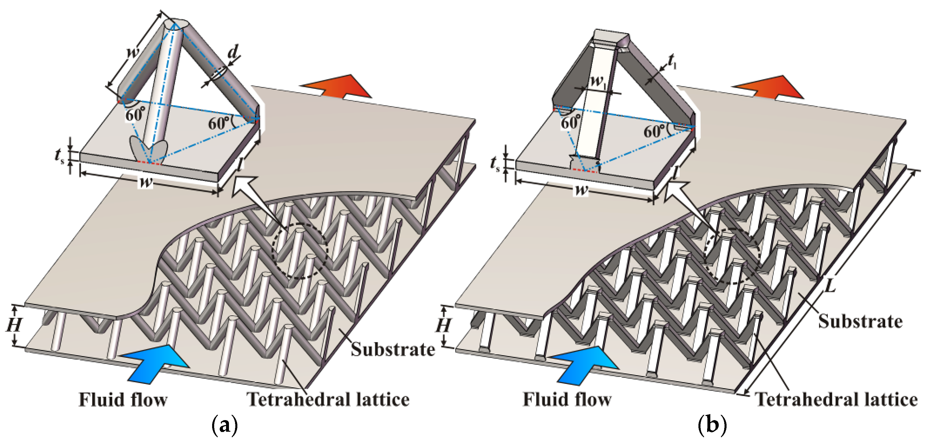
In light of the geometrical symmetry of the sandwich panels, only ten half-unit cells and the corresponding fluid around them are considered, as detailed in
Figure 3. To improve the numerical stability, two empty channels with a lengths of
l and 3
l, respectively, are configured upstream and downstream of the sandwich panel. It should be mentioned that the lattice core fabricated by the metal sheet folding method is modeled by using Sheet Metal Tools in Solidworks™, which can well represent the in-situ morphology.
The flow and heat transfer associated with the above sandwich panels are governed by the conservation of mass, momentum, and energy. To incorporate the turbulence effect, the shear stress transport (SST) turbulence model [
27] with a dimensionless wall distance (
y+) of less than 1.0 is adopted. The SST model has been proven to behave well for complex separated flow [
28], which is expected in the present sandwich panels. In this paper, the basic assumptions include: (a) the flow and heat transfer are steady-state; (b) the fluid is incompressible; (c) both the solid and fluid have constant thermo-physical properties; (d) the body force term in the momentum equation is neglected; and (e) the viscous dissipation term in the energy equation of fluid is neglected. The corresponding governing equations in a tensor form, which have been well documented in [
27,
28,
29], are summarized as follows:
Turbulent kinetic energy equation:
Turbulent frequency equation:
In the above equations, Vi (i = 1, 2, 3) denotes the three velocity components in the Cartesian coordinate system; xi (i = 1, 2, 3) refers to the Cartesian coordinate components; ρf is the density of the fluid; p is the static pressure; μf is the dynamic viscosity of the fluid; μt is the turbulent viscosity; Tf denotes the fluid temperature; kf is the thermal conductivity of the fluid; cpf is the specific heat of the fluid; Prt is the turbulent Prandtl number; Ts is the solid temperature; k is the turbulent kinetic energy; Pk refers to the production rate of turbulent kinetic energy due to fluid viscosity; ω is the turbulent frequency; F1 is a non-dimensional blending function; and the other symbols are the model constants.
In Equations (2) to (5), the turbulent viscosity (
μt) and turbulence production rate (
Pk) are separately defined as:
In Equations (6) and (7), the strain rate
S′ and the dimensionless function
F2 are separately defined as:
In Equation (9),
y′ denotes the minimum distance from an arbitrary point to its surrounding solid walls. The blending function
F1 is defined as:
In Equation (10), the term
CDkω is defined as:
In Equations (4) and (5), the coefficients
α3,
β3,
σk3, and
σω3 are separately calculated as follows:
The model constants in the above equations are summarized in
Table 2.
For a given mass flow rate of the working fluid (i.e., air in the present study), fully developed isothermal flow between two parallel plates is first simulated; for brevity, the details of this simple model are not shown here. Then the obtained flow field in conjunction with a constant static temperature (Tin) of 298.15 K is specified at the inlet of the computational domain as the inlet boundary condition. The mass flow rate is specified at the outlet to ensure mass conservation. The side surfaces of both the fluid and solid domains are set to be symmetric. A constant heat flux (q″) of 8000 W/m2 is applied to the outer surface of the bottom substrate, while the other walls are set to be adiabatic. For the interface between the solid and fluid domains, conservative interface flux and no-slip conditions are adopted.
The details of the numerical simulations are summarized in
Table 3. For comparison between the two different sandwich panels, the height of the lattice core (
H) is selected as the characteristic length scale; correspondingly, the Reynolds number in
Table 3 is defined as:
where
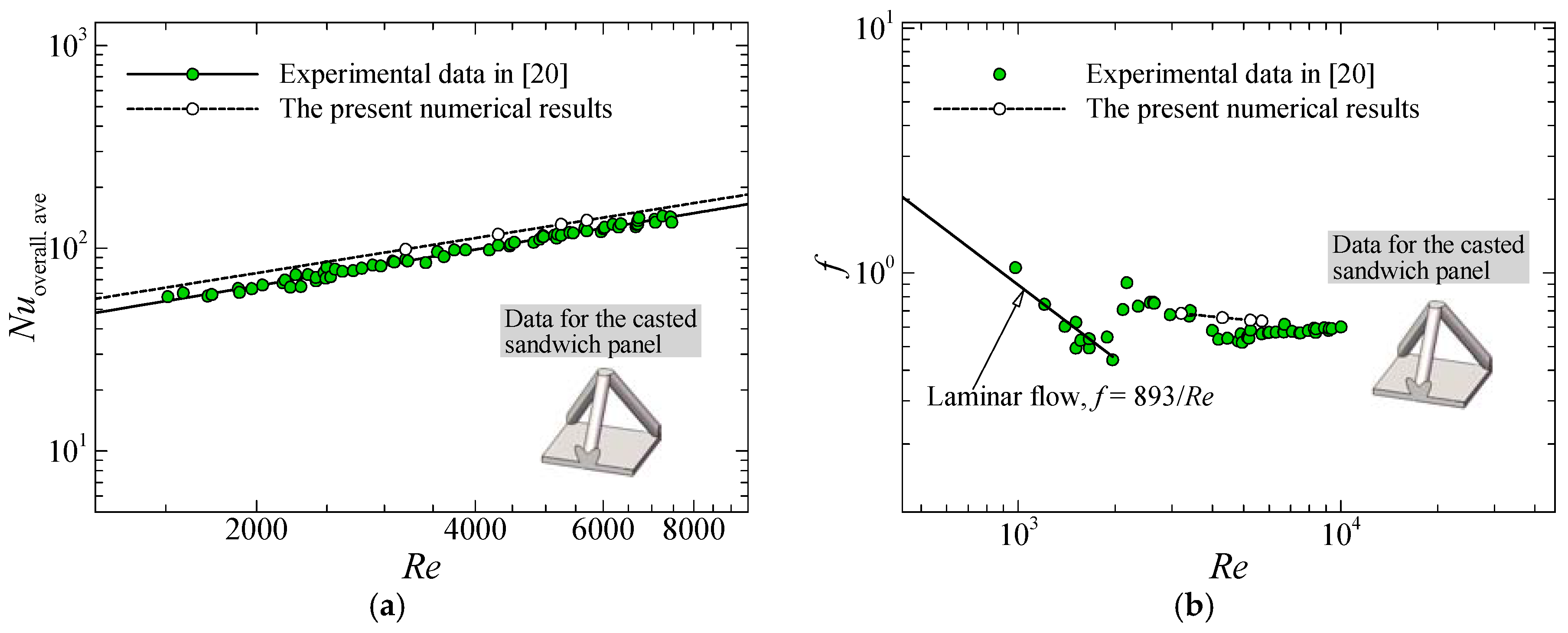
Um is the mean velocity along the channel height at the inlet of the computational domain. According to [
20], the flow considered in the present study is fully turbulent.
3.2. Numerical Methods
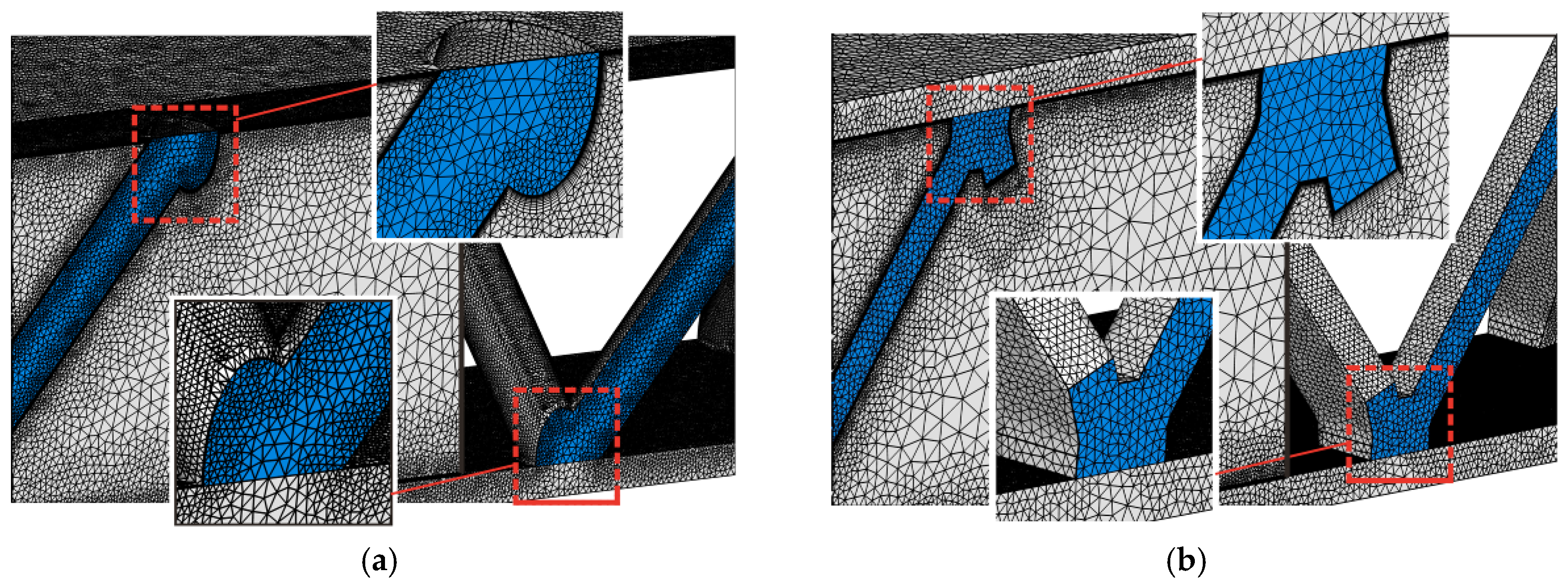
Due to the geometrical complexity of the present metallic lattices, an unstructured mesh composed of tetrahedral and prism elements is adopted to discretize both the solid and fluid domains as shown in
Figure 4. Fine meshes incorporating nine layers of prism elements are generated near all no-slip walls to well resolve the flow and thermal boundary layers; the height of the first layer of elements away from the solid walls is set to be 0.01 mm. To save computational cost, relatively coarse mesh is adopted for regions away from the walls. A smooth transition of the mesh is ensured to minimize numerical error.
The conjugate flow and heat transfer problem is solved in the commercial software package ANSYS CFX 15.0 (ANSYS Inc., Canonsburg, PA, USA) based on the finite volume method and time-marching algorithm. The fluid is assumed to be incompressible and has constant thermo-physical properties as given in
Table 3. A high resolution scheme and a central difference scheme are selected to discretize the advection terms and the diffusion terms in the governing equations, respectively. The solution is thought to be converged when the normalized residuals of all the governing equations are less than 10
−5. Correspondingly, the average temperature on the heated solid wall and the friction factor almost remain unchanged, with a variation less than 0.1%.
3.3. Mesh Independency
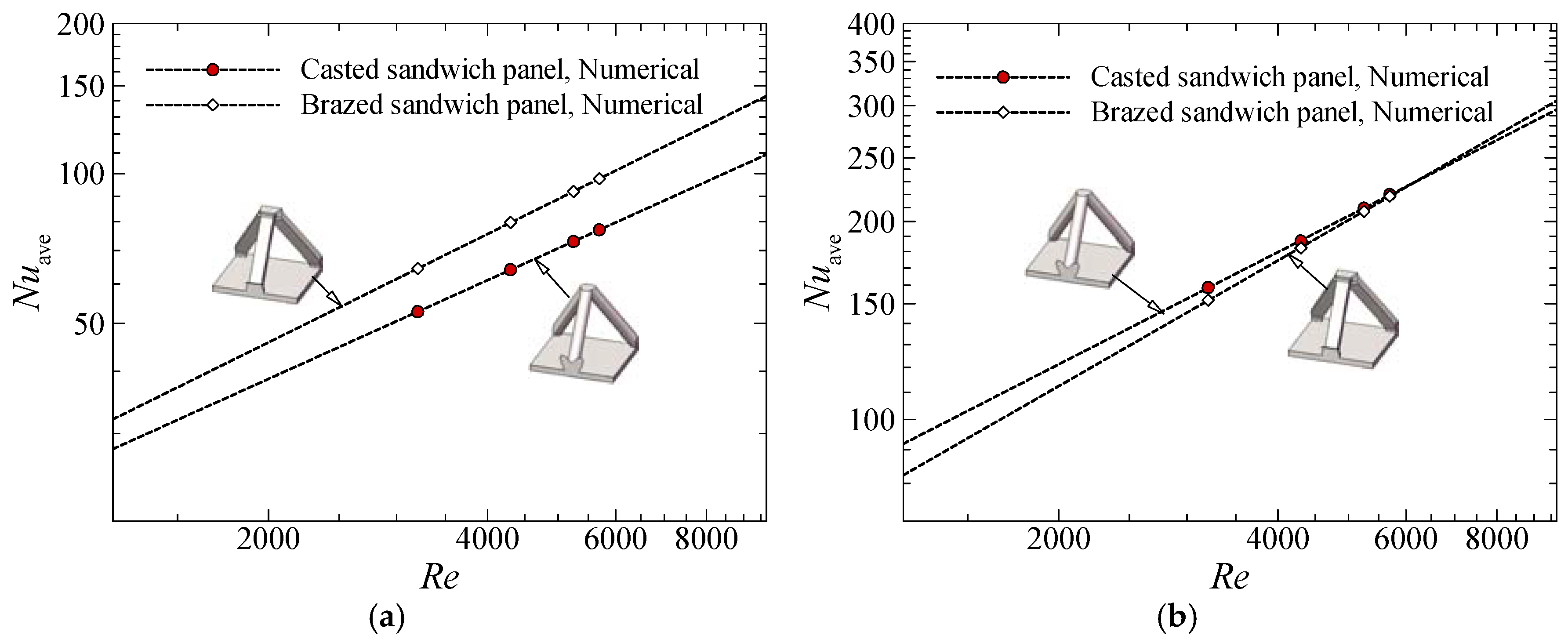
For the mesh sensitivity evaluation, two dimensionless parameters are defined. First, the overall Nusselt number (
Nuoverall) as an index of heat transfer is defined as:
The overall heat transfer coefficient (
hoverall) for each unit cell is defined as:
where
Twm is the inner surface temperature at the center of the substrate corresponding to each unit cell and
Tfb is the local bulk mean fluid temperature, which can be calculated based on the energy balance as:
where
yL is the distance between the inlet and the target point along the flow direction.
Second, the friction factor (
f) as an evaluation index of the pressure drop is defined as:
where Δ
p is the pressure drop through the sandwich panel and
L is the length of the sandwich panel along the flow direction as previously shown in
Figure 2.
For the casted sandwich panel, the mesh sensitivity is examined at the highest Reynolds number (i.e., 5700) within the range of 3209–5700 considered in the present study. Three sets of meshes with 7,649,638, 13,666,657, and 18,690,337 elements are separately generated. As revealed by
Table 4, the corresponding overall Nusselt number and the friction factor from the last two meshes show a discrepancy less than 1%, which is acceptable. Therefore, the mesh with 13,666,657 elements is used for all subsequent simulations. For the brazed sandwich panel, based on our previous experience during simulating a more complex X-type lattice cored sandwich panel [
18], the mesh with 21,4450,432 elements is sufficient to obtain a mesh-independent solution.


