Estimating Lithium-Ion Battery State of Charge and Parameters Using a Continuous-Discrete Extended Kalman Filter

Abstract

A real-time determination of battery parameters is challenging because batteries are non-linear, time-varying systems. The transient behaviour of lithium-ion batteries is modelled by a Thevenin-equivalent circuit with two time constants characterising activation and concentration polarization. An experimental approach is proposed for directly determining battery parameters as a function of physical quantities. The model’s parameters are a function of the state of charge and of the discharge rate. These can be expressed by regression equations in the model to derive a continuous-discrete extended Kalman estimator of the state of charge and of other parameters. This technique is based on numerical integration of the ordinary differential equations to predict the state of the stochastic dynamic system and the corresponding error covariance matrix. Then a standard correction step of the extended Kalman filter (EKF) is applied to increase the accuracy of estimated parameters. Simulations resulting from this proposed estimator model were compared with experimental results under a variety of operating scenarios—analysis of the results demonstrate the accuracy of the estimator for correctly identifying battery parameters.

1. Introduction

The crisis in Syria has deprived many of continuous and permanent access to electrical networks, so daily needs must be met through electrical energy storage, such as lead-acid and lithium-ion batteries. Given their importance, we have investigated means to maximize efficient monitoring, operation and management of battery resources.

To carry out this work, we chose lithium-ion technology. It is currently widely used in Syria to power portable electronics, such as laptop computers charged via solar bags. Moreover, compared with older battery technologies, lithium-ion batteries offer relatively high voltage, high specific energy, high specific power, no memory effect, and low self-discharge rates during storage.

An accurate model of battery dynamics should take into account multiple coefficients, such as open-circuit voltage, discharge rate, power, state of charge (SOC) and temperature.

However, it is difficult to determine or estimate battery parameters, because they are interdependent and vary over time and use. Many battery models are used to represent the battery behaviour. The most commonly used models can be divided into two categories: the electrochemical models and the electrical equivalent circuit models. The electrochemical models utilize a set of coupled non-linear differential equations to describe the pertinent transport, thermodynamic, and kinetic phenomena. The dynamical behaviour of a lithium-ion battery can be simulated correctly using the Warburg diffusion impedance with complex electrical equivalent circuits [1,2,3]. However, estimating the parameters of this sophisticated model usually requires an electrochemical impedance spectrometry (EIS). EIS data are analysed by fitting to a complex electrical equivalent circuit model for different values of the SOC and the temperature.

A big capacitor with series resistance can be selected to calculate dynamic terminal voltage of the battery. Later, a model with two capacitors in parallel was developed consisting of a double layer capacitor, a bulk capacitor, a charge transfer resistance and a terminal resistance [4]. Recently, the dual polarization model has been commonly used [5,6,7,8,9].

There are a lot of SOC estimation methods. The commonly used methods can be generally classified into four categories, namely, the direct discharge method, the Ampere-Hour counting method, the voltage/impedance-based method, and model-based filter methods [8,10,11,12]. The extended Kalman filter (EKF) is widely used for estimating the SOC and other battery parameters related to the SOC [13,14,15].

This paper proposes an experimental approach for identifying battery parameters. An EKF estimator was developed based on the Thevenin equivalent battery circuit. This recursive method can be used in real time to eliminate measurement and process noise. This hybrid approach, which is applied here to a continuous system with discrete measurements, is particularly suitable for battery systems [16,17,18].

2. Dynamical Model of Battery

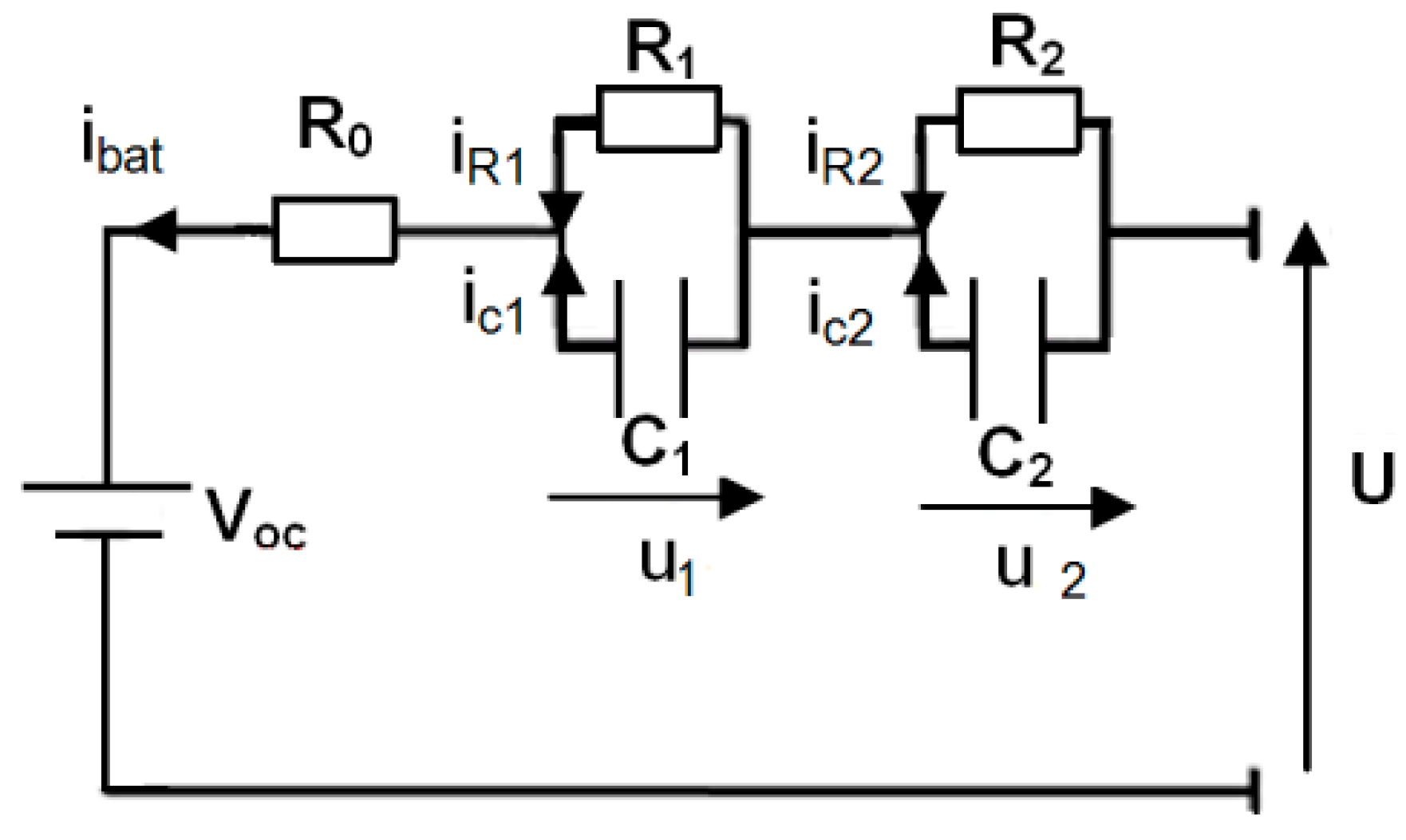
In order to describe the dynamic behaviour of a battery, we use the Thevenin equivalent circuit (dual polarization) shown in Figure 1 [19,20,21]. This battery equivalent circuit consists of two time constants ${\tau }_1=R_1{C}_1$ and ${\tau }_2=R_2{C}_2$. The constant ${\tau }_1$ characterizes the activation polarization while the constant ${\tau }_2$ characterizes the concentration polarization.

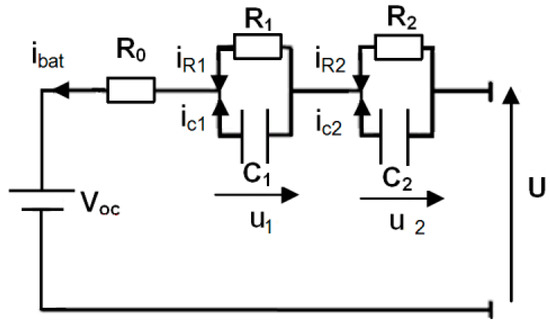
Figure 1. Thevenin equivalent circuit.

The elements of the battery equivalent circuit depicted in Figure 1 are as follows: $V_{oc}$ is the open-circuit voltage, $R_0$ is the ohmic resistance of the battery's collectors and electrodes, $i_{bat}$ is the charge/discharge current and $U$ represents the terminal voltage of the battery cell. As shown in Figure 1, the current $i_{bat}$ flowing through resistance $R_0$ can be expressed by the following equation:

$$i_{bat}=i_{R_1}+i_{C_1}=\frac{u_1}{R_1} +C_1\cdot \frac{{\mathrm{d}u}_1}{\mathrm{d}t}$$

(1)

Equation (1) can be rewritten as:

$$R_1\cdot i_{bat}=u_1+R_1\cdot C_1\cdot \frac{{\mathrm{d}u}_1}{\mathrm{d}t}$$

(2)

where $u_1$ is the voltage drop due to activation polarization. Similarly, we can write the following equation in the second circuit $R_2{C}_2$,

$$R_2\cdot i_{bat}=u_2+R_2\cdot C_2\cdot \frac{{\mathrm{d}u}_2}{\mathrm{d}t}$$

(3)

where $u_2$ is the voltage drop due to mass transport (concentration polarization).

Therefore, the terminal voltage $U$ of the cell is determined by the open-circuit voltage $V_{oc}$ and the different drops of voltage as given by Equation (4).

$$U=V_{oc}+u_1+u_2+R_0\cdot i_{bat}$$

(4)

3. Studied Battery and Experimental Device

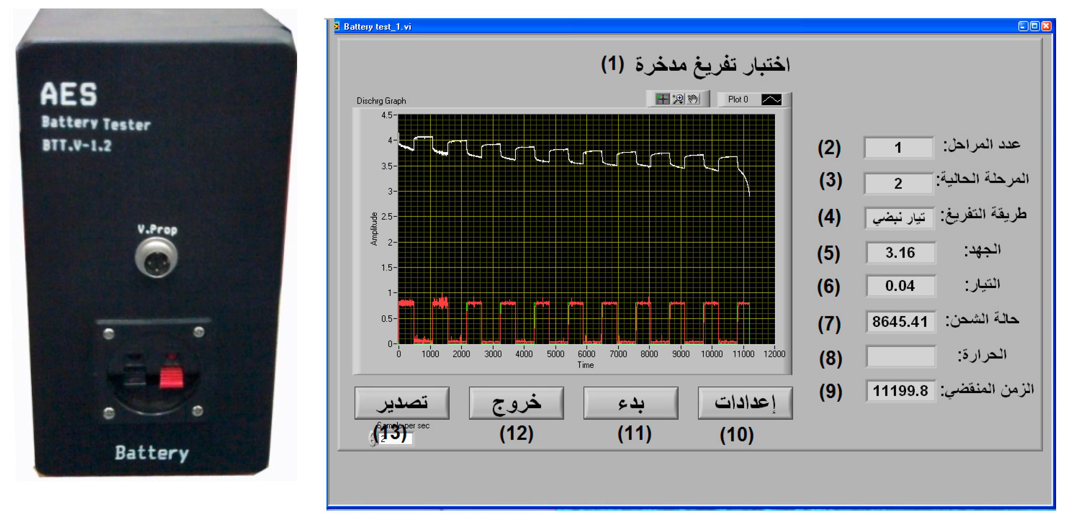
In order to measure the parameters of the battery, a single cell of Li-ion battery (2.15 Ah, 3.7 V) is used [22]. Appendix A provides detailed parameters of the battery cell. Figure 2 shows a photo of the charge/discharge experimental device which we programmed using LabView.

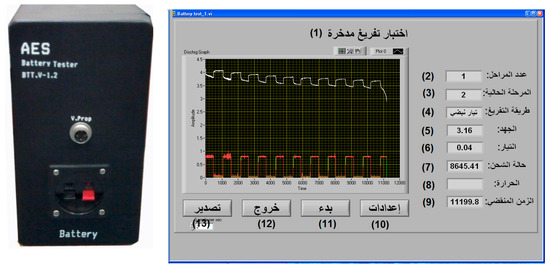
Figure 2. Experimental device and user interface (1) battery discharge test (2) step number (3) current step (4) discharge method (5) voltage (6) current (7) state of charge (8) temperature (9) elapsed time (10) edit (11) start (12) exit (13) export.

4. Determining Open-Circuit Voltage as a Function of SOC

Accuracy of the Thevenin circuit relies on diverse conditions, especially the $\mathrm{SOC}$. To estimate the $\mathrm{SOC}$ during the charging/discharging of a battery, the Ampere-Hour counting (AHC) technique is used. It is the most common technique for calculating the $\mathrm{SOC}$. The $\mathrm{SOC}$ variation during charge/discharge can be calculated as [7,23]:

$$\frac{\mathrm{d}}{\mathrm{d}t}\mathrm{SOC}=\eta \cdot \frac{i_{bat}-I_0}{Q}$$

(5)

where, $Q$ is the initial ampere-hour of battery, $I_0$ is the current consumed by the parasitic reactions, $\eta$ is the Coulombic efficiency, which is a function of the current and the temperature. Coulombic efficiency is the ratio of the Ampere-hours removed from a battery during discharge to the Ampere-hours required to restore the initial capacity [24]. Before each discharge test, the battery is fully charged for more than 24 hours with the floating technique. This allows us to neglect the losses due to parasitic reactions [25].

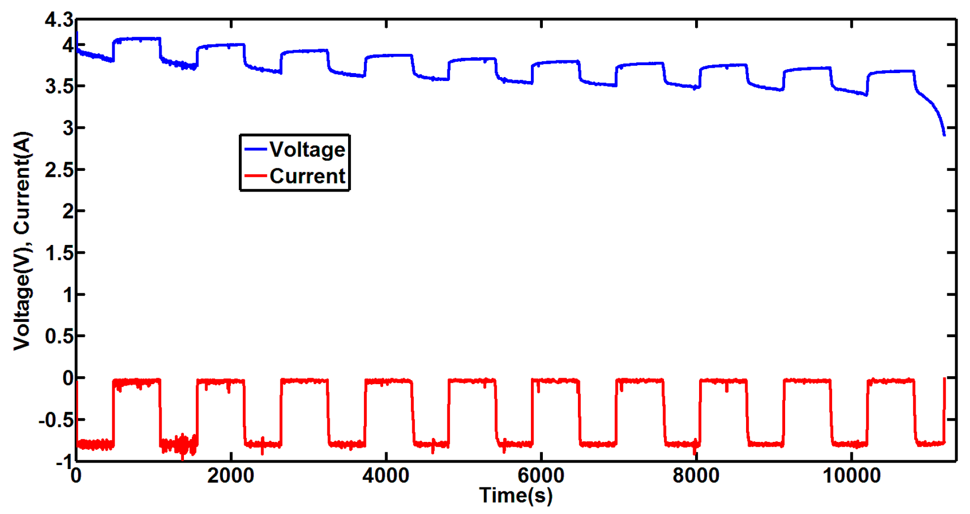
The first parameter in the model shown in Figure 1 is the open-circuit voltage $V_{oc}$. The $V_{oc}$ is usually measured at various $\mathrm{SOC}$ points as the steady-state open circuit terminal voltage. For each $\mathrm{SOC}$ point, this measurement can take many days, but in our research, we used a quick measurement technique. To measure $V_{oc}$ at various $\mathrm{SOC}$ points, the battery was discharged by injecting successive current pulses. The battery cell was discharged with a pulse current of 0.8 A (0.37 C) from full charge ($\mathrm{SOC}=100\%$) to cut-off voltage ($\mathrm{SOC}=0\%$) [22]. C-rate is the discharge rate of the battery relative to its capacity. This current pulse has 480 s on-time and 600 s off-time. Figure 3 shows the pulse discharge current and the battery terminal voltage. The experimental data was obtained at a room temperature of 25 °C.

Figure 3. Discharge current and battery terminal voltage.

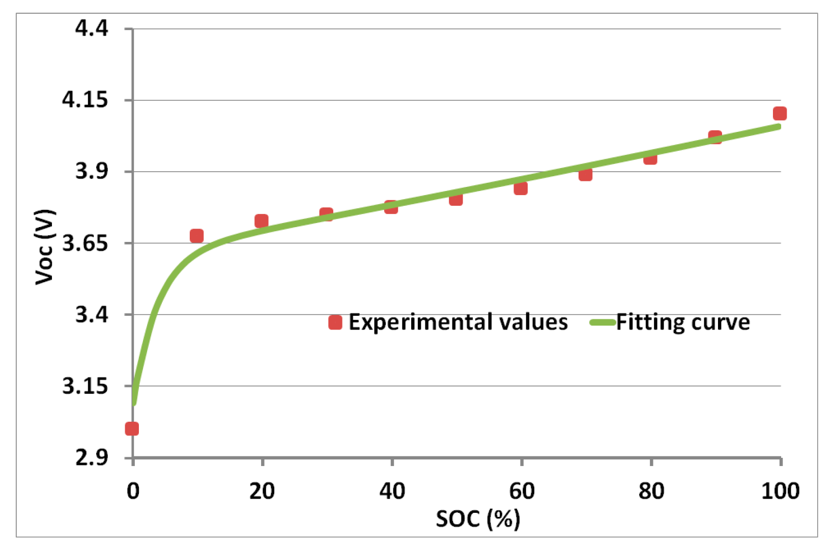
It was considered that each pulse current discharged the battery by 10%. The open-circuit voltage $V_{oc}$ was measured at equilibrium potential. The points in Figure 4 show the $V_{oc}$ versus $\mathrm{SOC}$. The relation between the $V_{oc}$ and the $\mathrm{SOC}$ is non-linear. The curve is steep at the beginning (for $\mathrm{SOC}$ lower than 20%) and then linear [26,27,28].

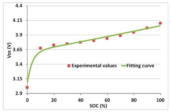
Figure 4. Experimental and fitting result of $V_{oc}$ versus state of charge ($\mathrm{SOC}$).

It is important to include the variation of $V_{oc}$ as a function of $\mathrm{SOC}$ in the whole battery model. The experimental value is interpolated by a fitting technique (using software FindGraph). The resulting fitting function is given by:

$$V_{OC} \left(\mathrm{SOC}\right)=a_v\cdot \exp (b_v\cdot \mathrm{SOC})+d_v\cdot \exp (c_v\cdot \mathrm{SOC})$$

(6)

Table 1 represents the relative fitting errors for battery parameters.

Table 1. Fitting error for battery parameters.

Parameter	Error (Root Mean Square)
$\mathsf{\Delta }{R}_1$	1.5%
$\mathsf{\Delta }{C}_1$	2.0%
$\mathsf{\Delta }{R}_2$	1.3%
$\mathsf{\Delta }{C}_2$	2.3%
$\mathsf{\Delta }{V}_{oc}$	1.2%

5. Identification of Model Parameters as a Function of SOC

Figure 5 shows the typical voltage response of a battery. The voltage drop may be divided into two parts. The first ($\mathsf{\Delta }{V}_1$) is a vertical straight drop largely dependent on the battery’s ohmic resistance $R_0$. It can be estimated by [29]:

$$R_0=\frac{\mathsf{\Delta }{V}_1}{i_{bat}}$$

(7)

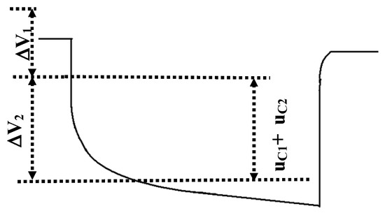
Figure 5. Single pulse of voltage response.

The second ($\mathsf{\Delta }{V}_2$) is the voltage drop based on resistances $R_1$ and $R_2$. It is experimentally difficult to measure the time constants for activation and concentration separately. Moreover, some simplified hypotheses may lead to important errors. As the experimental results show, resistance $R_0$ varies slightly with SOC. This concurs with publications [8,29,30] showing that other parameters of the model vary non-linearly versus $\mathrm{SOC}$.

In a single pulse, the value of the current $i_{bat}$ is either constant or zero. Therefore, the solutions for Equations (2) and (3) will be as follows:

$$u_1=i_{bat}\cdot R_1\cdot (1-\exp (-t/{\tau }_1\left)\right)$$

(8a)

$$u_2=i_{bat}\cdot R_2\cdot (1-\exp (-t/{\tau }_2\left)\right)$$

(8b)

This means that during discharge, each voltage can be represented by an exponential. We suggest using regression analysis to fit the voltage experimental data with two exponentials. Based on the experimental data, a regression analysis is conducted at each $\mathrm{SOC}$ separately, and for different pulse currents (0.8, 1.2 and 1.5 A; 0.37, 0.56 and 0.7 C). Through this approach, the elements of the battery equivalent circuit can be determined.

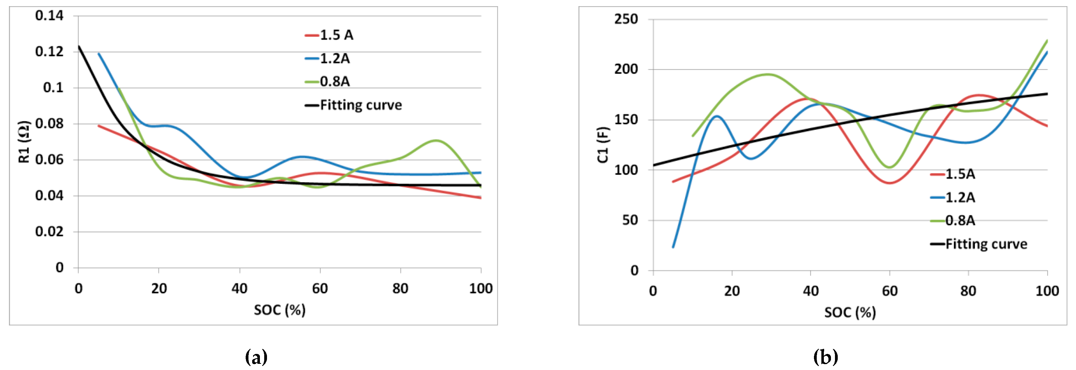
This approach is repeated for each pulse where it is supposed that the elements $R_1$, $C_1$, $R_2$ and $C_2$ are independent of $\mathrm{SOC}$ only for the related pulse. Figure 6 represents the values of the resistance $R_1$ and the capacitance $C_1$ as a function of $\mathrm{SOC}$ for three values of the discharge current.

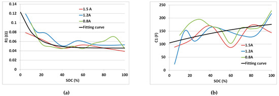
Figure 6. Values of activation parameters versus $\mathrm{SOC}$ for different discharge currents (a) resistance $R_1$ (b) capacitance $C_1$.

The resistance $R_1$ decreases roughly with the increase of $\mathrm{SOC}$. Using fitting, the average value of $R_1$ can be expressed by an exponential function as follows:

$$R_1\left(\mathrm{SOC}\right)=a_{r1}+b_{r1}\cdot \exp (c_{r1}\cdot \mathrm{SOC})$$

(9a)

$$C_1\left(\mathrm{SOC}\right)=a_{c1}\cdot {\mathrm{SOC}}^2+b_{c1}\cdot \mathrm{SOC}+c_{c1}$$

(9b)

A polynomial is selected to fit the experimental values of the capacitance $C_1$.

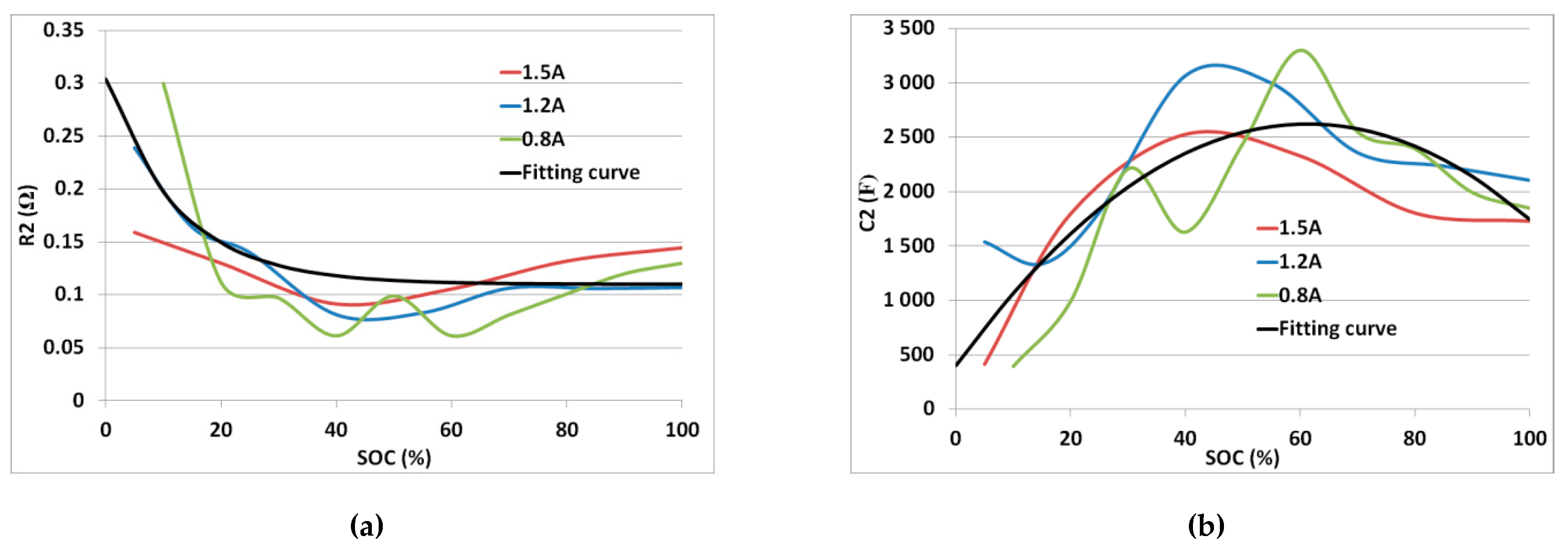
The values of the resistance $R_2$ and of the capacitance $C_2$ as a function of $\mathrm{SOC}$ are shown in Figure 7 for different discharge currents. It can be seen where $\mathrm{SOC}$ is less than 20%, resistance $R_2$ is higher.

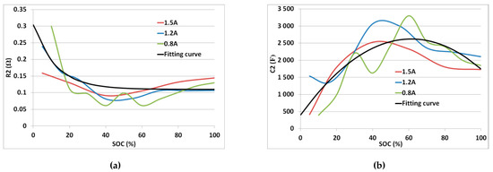
Figure 7. Values of concentration parameters versus $\mathrm{SOC}$ for different discharge currents (a) resistance $R_2$ (b) capacitance $C_2$.

Similarly, we found that the both parameters $R_2$ and $C_2$ can be expressed as:

$$R_2\left(\mathrm{SOC}\right)=a_{r2}+b_{r2}\cdot \exp (c_{r2}\cdot \mathrm{SOC})$$

(10a)

$$C_2\left(\mathrm{SOC}\right)=a_{c2}\cdot {\mathrm{SOC}}^4+b_{c2}\cdot {\mathrm{SOC}}^3+c_{c2}\cdot {\mathrm{SOC}}^2+d_{c2}\cdot \mathrm{SOC}+e_{c2}$$

(10b)

where $\mathrm{SOC}$ is at or above 30%, variation is low for resistances and high for capacitances.

6. Determining the Battery Coulombic Efficiency

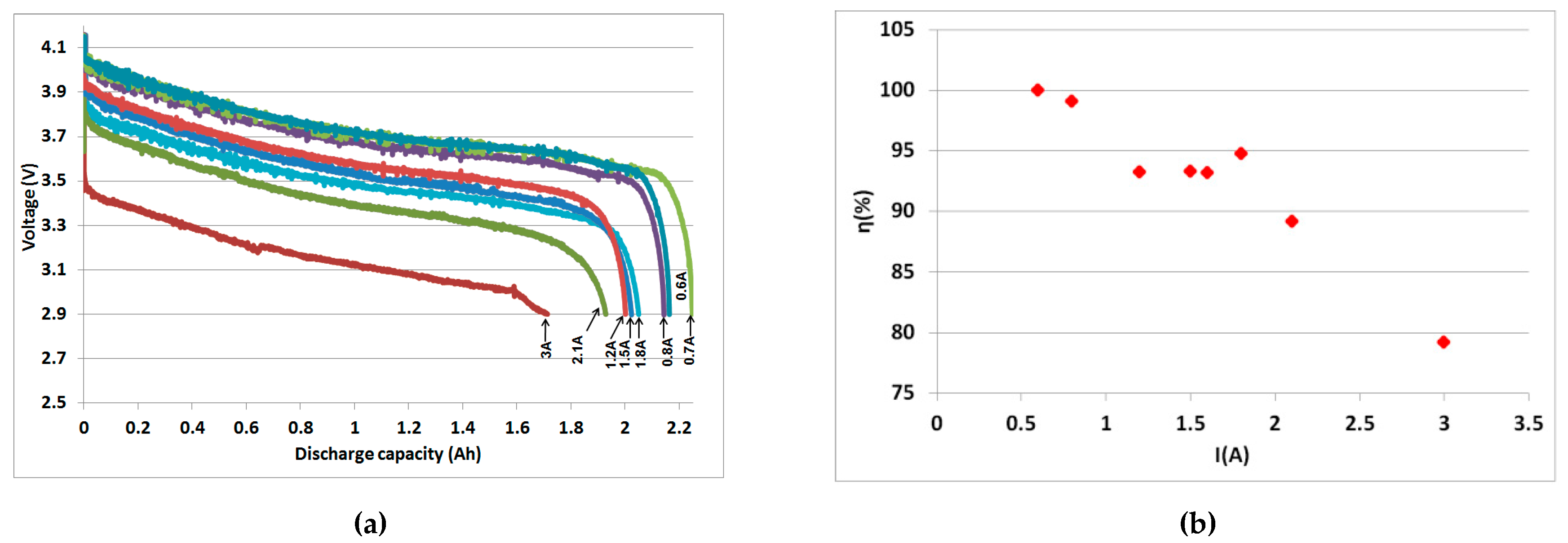
The battery is discharged at various constant currents in the range of 0.6–3 A (0.2–1.4 C). The experimental results are shown in Figure 8. The discharge rate of the battery substantially affects the voltage curve—as it increases, the voltage curve shifts downward significantly. For a high discharge current (3 A), the discharge curve is deformed and the battery capacity decreases markedly.

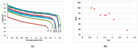
Figure 8. Battery capacity at different discharge currents (a) voltage response (b) Coulombic efficiency.

The battery Coulombic efficiency will decrease as the discharge rate increases, as shown in Figure 8b. There is an approximately linear relationship between the discharge current and the Coulombic efficiency. As can be noticed in Figure 8, the effect of discharge rate on useful battery capacity is clear. It is still lower in Li-ion batteries than in lead acid batteries, however, due to the very fast redox reactions in Li-ion batteries [31].

Since phenomena in battery systems are influenced by temperature, the model adjusts for Coulombic efficiency variation [22,24].

7. Comparison between Simulation and Experimental Results

Using the previous equations, an extended battery model (EBM) was built with the MATLAB/SIMULINK environment. To compare the experimental and simulated results, several tests were carried out using pulse discharge currents. The results are as follows:

• Pulse discharge current of 0.8 A (presented in Figure 3): Figure 9a shows the comparison between the simulation and the experimental voltages. Figure 9b illustrates the small size of the simulation error, hardly reaching 0.06 V and remaining at less than 1% virtually throughout the test.
  

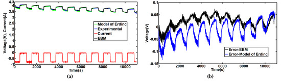  Figure 9. Simulation and experimental curves for 0.8 A current (a) voltages and current, (b) voltages error.
• Pulse discharge current of 1 A (0.47 C) (180 s on-time and 60 s off-time): Figure 10a overlays the simulated voltage and the experimental voltage curves, while Figure 10b illustrates the small error rate.
  

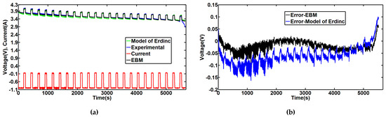  Figure 10. Simulation and experimental curves for 1A current (a) voltages and current, (b) voltages error.
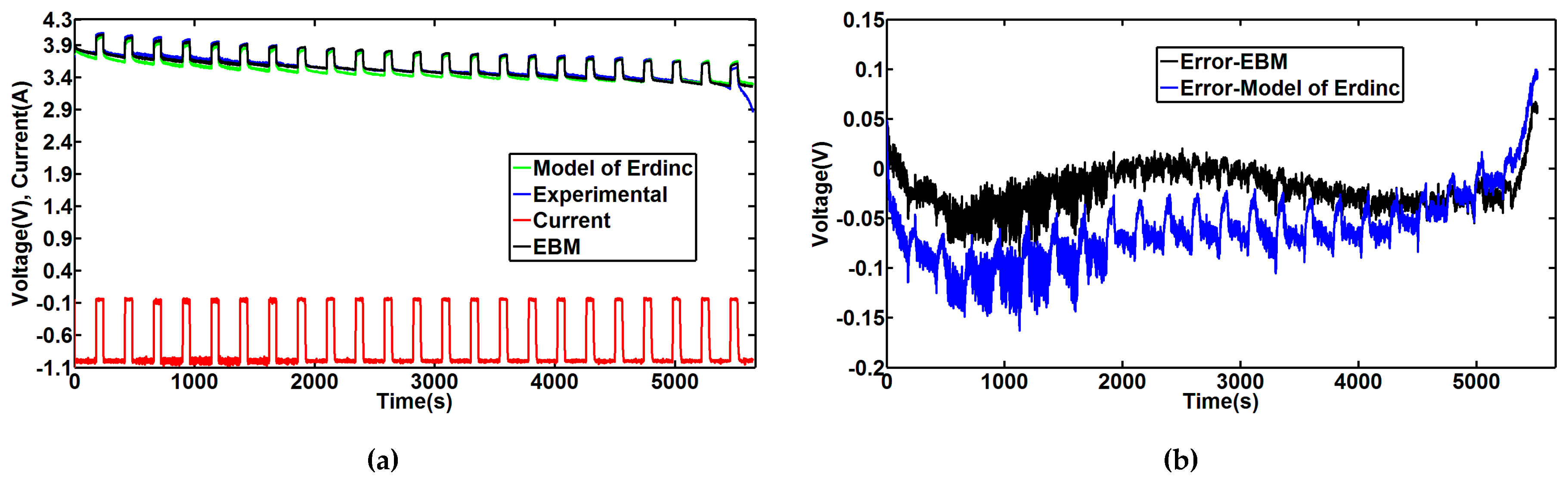
• Pulse discharge current of 1.5 A (0.7 C) (480 s on-time and 600 s off-time): The comparison between the simulation and the experimental voltages is represented in Figure 11a. It can be observed in Figure 11b that the error rate, while still low, is slightly higher at this higher pulse discharge current, especially as the battery reaches full discharge.
  

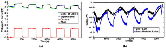  Figure 11. Simulation and experimental curves for 1.5 A current (a) voltages and current, (b) voltages error.

The previously proposed model was used to simulate the dynamic characteristics of the lithium battery. The model’s relative accuracy was validated across a variety of voltage profiles. As the discharge current increased, however, the EBM error increased slightly. And as the battery approached full discharge, an important error emerged. This error can be explained by the sharp open-circuit voltage drop that slightly influences battery runtime. The proposed EBM model is also compared with the Erdinc model [6] on Figure 9, Figure 10 and Figure 11. These Figures clearly show that since it considers that the battery parameters slightly vary with SOC, the Erdinc model produces simulation results that are farther from the experimental results than the EBM model.

We will now examine additional steps to estimate the parameters of a real battery in real time.

8. Estimating Battery Parameters Using an Extended Kalman Filter

The Ampere Hour counting (AHC) technique used for estimating $\mathrm{SOC}$ can be accurate, but it can accumulate errors with time. Its accuracy depends very much on determining initial $\mathrm{SOC}$, and it is subject to measurement noise [32,33]. To improve accuracy, an extended Kalman filter (EKF) is used. It is a nonlinear optimum state estimation method based on a continuous-time model and on discrete-time measurements. A continuous-discrete extended Kalman estimator of the lithium-ion battery is derived from the model previously built to determine the $\mathrm{SOC}$ and other parameters of a battery with less error.

$u_1$, $u_2$, $\mathrm{SOC}$, $1/{\tau }_1$, $1/C_1$, $1/{\tau }_2$, $1/C_2$ and $R_0$ are chosen as state-variables: $x_1=u_1$, $x_2=u_2, x_3=\mathrm{SOC}$, $x_4=1/{\tau }_1$, $x_5=1/C_1$, $x_6=1/{\tau }_2$, $x_7=1/C_2$, $x_8=R_0.$ We have chosen this set of parameters because it simplifies the extended Kalman filter estimator. From Thevenin circuit equations of Figure 1 and Equation (5) (see Appendix B), we can write the state equations as follows:

$${\dot{x}}_1=-x_4\cdot x_1+x_5\cdot i_{bat}$$

(11a)

$${\dot{x}}_2=-x_6\cdot x_2+x_7\cdot i_{bat}$$

(11b)

$${\dot{x}}_3=\eta (i_{bat})\cdot \frac{1}{Q}\cdot i_{bat}$$

(11c)

Determination of battery parameters as a function of $\mathrm{SOC}$ allows us to develop the extended Kalman filter observer to identify parameters in real-time. The derivation of time equations for the other state-variables is summarised below.

The time equation for $x_4$ can be developed from Equation (12a).

$${\dot{x}}_4=\frac{{dx}_4}{{dx}_3}\cdot {\dot{x}}_3$$

(12a)

Equation (12a) can be rewritten replacing $x_4$ by $1/{\tau }_1$ as:

$${\dot{x}}_4=\left(-\frac{\frac{{\mathrm{d}\tau }_1}{{\mathrm{d}x}_3}(x_3)}{{\tau }_1{(x_3)}^2}\right)\cdot \frac{\eta \cdot i_{bat}}{Q}=-x_4^2\cdot \frac{{\mathrm{d}\tau }_1}{{\mathrm{d}x}_3}(x_3)\cdot \frac{\eta \cdot i_{bat}}{Q}$$

(12b)

The derivative of the constant ${\tau }_1$ with respect to $x_3$ can be calculated as:

$$\frac{{\mathrm{d}\tau }_1}{{\mathrm{d}x}_3}(x_3)=\frac{{\mathrm{d}R}_1}{{\mathrm{d}x}_3}(x_3)\cdot C_1(x_3)+R_1(x_3)\cdot \frac{{\mathrm{d}C}_1}{{\mathrm{d}x}_3}(x_3)$$

(12c)

Then, Equation (12b) can be rewritten as:

$${\dot{x}}_4=-x_4^2\cdot \left(\frac{{\mathrm{d}R}_1}{{\mathrm{d}x}_3}(x_3)\cdot \frac{1}{x_5}+R_1(x_3)\cdot \frac{{\mathrm{d}C}_1}{{\mathrm{d}x}_3}(x_3)\right)\cdot \frac{\eta \cdot i_{bat}}{Q}$$

(12d)

The resistance $R_1$ is replaced as:

$$R_1(x_3)=\frac{x_5}{x_4}$$

(12e)

Finally, variable $x_4$ can be expressed as follows:

$${\dot{x}}_4=-x_4^2\cdot \left(\frac{{\mathrm{d}R}_1}{{\mathrm{d}x}_3}(x_3)\cdot \frac{1}{x_5}+\frac{x_5}{x_4}\cdot \frac{{\mathrm{d}C}_1}{{\mathrm{d}x}_3}(x_3)\right)\cdot \frac{\eta \cdot i_{bat}}{Q}$$

(12f)

Similarly, the time equation for $x_5$ can developed as follows:

$${\dot{x}}_5=\frac{{\mathrm{d}x}_5}{{\mathrm{d}x}_3}\cdot {\dot{x}}_3=\left(-\frac{\frac{{\mathrm{d}C}_1}{{\mathrm{d}x}_3}(x_3)}{C_1{(x_3)}^2}\right)\cdot \frac{\eta \cdot i_{bat}}{Q}=-x_5^2\cdot \frac{{\mathrm{d}C}_1}{{\mathrm{d}x}_3}(x_3)\cdot \frac{\eta \cdot i_{bat}}{Q}$$

(13)

Likewise, we can compute variables $x_6$ and $x_7$ in the same manner.

$${\dot{x}}_6=-x_6^2\cdot \left(\frac{{\mathrm{d}R}_2}{{\mathrm{d}x}_3}(x_3)\cdot \frac{1}{x_7}+\frac{x_7}{x_6}\cdot \frac{{\mathrm{d}C}_2}{{\mathrm{d}x}_3}(x_3)\right)\cdot \frac{\eta \cdot i_{bat}}{Q}$$

(14)

$${\dot{x}}_7=-x_7^2\cdot \frac{{\mathrm{d}C}_2}{{\mathrm{d}x}_3}(x_3)\cdot \frac{\eta \cdot i_{bat}}{Q}$$

(15)

The time derivative of variable $x_8$ is assumed to be zero.

$$\frac{{\mathrm{d}x}_8}{\mathrm{d}t}=0$$

(16)

In such a case, we can use a continuous-discrete extended Kalman filter (CD-EKF). The system of interest is a continuous-time dynamic system with discrete-time measurements given by [34,35,36]:

$$\dot{x}=f(x(t), i_{bat}(t))+\nu (t)$$

(17a)

$$U(n\cdot T_s)=h(x(n\cdot T_s),i_{bat}(n\cdot T_s))+w_n$$

(17b)

where $v\left(t\right)$ is the unmeasured “process noise” which is assumed to be a continuous-time Gaussian zero-mean white noise of covariance matrix $q$; $w_n$ is the measurement noise which is assumed to be a discrete-time Gaussian zero-mean white noise of covariance matrix $R$; and $x_n=x({nT}_s)$, where $n$ is the sampling number; and $T_s$ is the sampling period. The $U$ and $i_{bat}$ are the output and input measurements.

The Kalman filter mainly involves two steps: prediction and measurement update. The predicted state $x$ and its covariance matrix $P$ is calculated by solving ordinary differential equations (ODE) in the form Equation (15) [37]:

$$\dot{\widehat{x}}=f(\widehat{x}(t), i_{bat}(t))$$

(18a)

$$\dot{P}(\widehat{x}(t))=F(\widehat{x}(t))\cdot P(t)+P(t).F{(\widehat{x}(t))}^T+q$$

(18b)

The dynamic matrix $F$ (the Jacobian matrix of partial derivatives of function $f$) can be computed:

$$F(\widehat{x}(t))=\frac{\partial f}{\partial x}(\widehat{x}(t),i_{bat}(t))=\left[\begin{array}{llllllll}{F}_{11}& 0& 0& F_{14}& F_{15}& 0& 0& 0\\ 0& F_{22}& 0& 0& 0& F_{26}& F_{27}& 0\\ 0& 0& 0& 0& 0& 0& 0& 0\\ 0& 0& F_{43}& F_{44}& F_{45}& 0& 0& 0\\ 0& 0& F_{53}& 0& F_{55}& 0& 0& 0\\ 0& 0& F_{63}& 0& 0& F_{66}& F_{67}& 0\\ 0& 0& F_{73}& 0& 0& 0& F_{77}& 0\\ 0& 0& 0& 0& 0& 0& 0& 0\end{array}\right]$$

(19)

where,

$$F_{11}=-x_4,F_{14}=-x_1, F_{15}=i_{bat}, F_{22}= -x_6, F_{26}=-x_2, F_{27}= i_{bat}$$

(20a)

$$F_{43}=x_4^2\cdot \left(2\times x_4\cdot {\left(\frac{{\mathrm{d}\tau }_1}{{\mathrm{d}x}_3}(x_3)\right)}^2-\frac{{\mathrm{d}}^2{\tau }_1}{\mathrm{d}{x}_3^2}(x_3)\right)\cdot \frac{\eta \cdot i_{bat}}{Q}$$

(20b)

$$F_{44}=-2\times x_4\cdot \frac{{\mathrm{d}\tau }_1}{{\mathrm{d}x}_3}(x_3)\cdot \frac{\eta \cdot i_{bat}}{Q}$$

(20c)

$$F_{45}=x_4\cdot \left(\frac{x_4}{x_5^2}\cdot \frac{{\mathrm{d}R}_1}{{\mathrm{d}x}_3}(x_3)-\frac{{\mathrm{d}C}_1}{{\mathrm{d}x}_3}(x_3)\right)\cdot \frac{\eta \cdot i_{bat}}{Q}$$

(20d)

$$F_{53}=x_5^2\cdot \left(2\times x_5\cdot {\left(\frac{{\mathrm{d}C}_1}{{\mathrm{d}x}_3}(x_3)\right)}^2-\frac{{\mathrm{d}}^2{C}_1}{\mathrm{d}{x}_3^2}(x_3)\right)\cdot \frac{\eta \cdot i_{bat}}{Q}$$

(20e)

$$F_{55}=-2\times x_5\cdot \frac{{\mathrm{d}C}_1}{{\mathrm{d}x}_3}(x_3)\cdot \frac{\eta \cdot i_{bat}}{Q}$$

(20f)

$$F_{63}=x_6^2\cdot \left(2\times x_6\cdot {\left(\frac{{\mathrm{d}\tau }_2}{{\mathrm{d}x}_3}(x_3)\right)}^2-\frac{{\mathrm{d}}^2{\tau }_2}{\mathrm{d}{x}_3^2}(x_3)\right)\cdot \frac{\eta \cdot i_{bat}}{Q}$$

(20g)

$$F_{66}=-2\times x_6\cdot \frac{{\mathrm{d}\tau }_2}{{\mathrm{d}x}_3}(x_3)\cdot \frac{\eta \cdot i_{bat}}{Q}$$

(20h)

$$F_{67}=x_6\cdot \left(\frac{x_6}{x_7^2}\cdot \frac{{\mathrm{d}R}_2}{{\mathrm{d}x}_3}(x_3)-\frac{{\mathrm{d}C}_2}{{\mathrm{d}x}_3}(x_3)\right)\cdot \frac{\eta \cdot i_{bat}}{Q}$$

(20i)

$$F_{73}=x_7^2\cdot \left(2\times x_7\cdot {\left(\frac{{\mathrm{d}C}_2}{{\mathrm{d}x}_3}(x_3)\right)}^2-\frac{{\mathrm{d}}^2{C}_2}{\mathrm{d}{x}_3^2}(x_3)\right)\cdot \frac{\eta \cdot i_{bat}}{Q}$$

(20j)

$$F_{77}=-2\times x_7\cdot \frac{{\mathrm{d}C}_2}{{\mathrm{d}x}_3}(x_3)\cdot \frac{\eta \cdot i_{bat}}{Q}$$

(20k)

The initial value of error matrix covariance $P_0$ and $q$ are given by:

$$P_0=\left[\begin{array}{llllllll}{P}_{110}& 0& 0& 0& 0& 0& 0& 0\\ 0& P_{220}& 0& 0& 0& 0& 0& 0\\ 0& 0& P_{330}& 0& 0& 0& 0& 0\\ 0& 0& 0& P_{440}& 0& 0& 0& 0\\ 0& 0& 0& 0& P_{550}& 0& 0& 0\\ 0& 0& 0& 0& 0& P_{660}& 0& 0\\ 0& 0& 0& 0& 0& 0& P_{770}& 0\\ 0& 0& 0& 0& 0& 0& 0& P_{880}\end{array}\right] q=\left[\begin{array}{llllllll}{q}_1& 0& 0& 0& 0& 0& 0& 0\\ 0& q_2& 0& 0& 0& 0& 0& 0\\ 0& 0& q_3& 0& 0& 0& 0& 0\\ 0& 0& 0& q_4& 0& 0& 0& 0\\ 0& 0& 0& 0& q_5& 0& 0& 0\\ 0& 0& 0& 0& 0& q_6& 0& 0\\ 0& 0& 0& 0& 0& 0& q_7& 0\\ 0& 0& 0& 0& 0& 0& 0& q_8\end{array}\right]$$

(21)

The values of these matrices are provided in Appendix A. The covariance matrix $q$ was computed through manual testing in MATLAB.

The two Equations (18a) and (18b) are solved simultaneously with the nonlinear ODE solver [38]. Equation (18b) is vectorised. Here, we implanted the filter (CD-EKF) in MATLAB with ODE45 Dormand-Prince variable-step differential equation solver because it implements the Runge-Kutta pair, one of the best methods for treating non-stiff general-form initial value problems for ODE. The integration is done in the interval [$t_{n-1}$, $t_n$] with the initial conditions: $\widehat{x}(t_{n-1})={\widehat{x}}_{n-1/n-1}$ and the error covariance matrix $P(t_{n-1})=P_{n-1/n-1}$. We compute the predicted estimate state ${\widehat{x}}_{n/n-1}=\widehat{x}(t_n)$ and the error covariance matrix $P_{n/n-1}=P(t_n)$ at time $t_n$ [37]. Then, we use the standard correction step of the EKF. Additionally, we calculate only the upper triangular part of the error covariance matrix including the main diagonal because of its symmetry. As a result, we have 44 equations (ODE) to solve with 44 unknown variables. Then the standard measurement update is applied at time ($t_n=n{T}_s$). The function $h$ deriving the observation equation is given by:

$$h(x,i_{bat})=V_{oc}(x_3)+x_1+x_2+x_8\cdot i_{bat}$$

(22)

The observation matrix $H$ can be calculated by:

$$H(x)=\frac{\partial h}{\partial x}(x,i_{bat})=\left[1 1 h_3(x_3) 0 0 0 0 i_{bat}\right]$$

(23a)

where,

$$h_3(x_3)=\frac{\partial V_{oc}}{\partial x_3}(x_3)=a_v\cdot b_v\cdot \exp (b_v\cdot x_3)+c_v\cdot d_v\cdot \exp (d_v\cdot x_3)$$

(23b)

The Kalman gain can be computed as:

$$K_n=P_{n/n-1}\cdot H{({\widehat{x}}_{n/n-1})}^T\cdot {S_n}^{-1}$$

(24a)

$$S_n=H({\widehat{x}}_{n/n-1})\cdot P_{n/n-1}\cdot H{({\widehat{x}}_{n/n-1})}^T+R$$

(24b)

where $R$ is the measurement noise covariance. As presented in Reference [39], Auger et al. proposed that the value of covariance $R$ can be set to one ($R=1$). The state estimation covariance is updated by:

$$P_{n/n}=(1-K_n\cdot H({\widehat{x}}_{n/n-1}))\cdot P_{n/n-1}$$

(25)

We use the Kalman gain to update the state estimation:

$${\widehat{x}}_{n/n}={\widehat{x}}_{n/n-1}+K_n\cdot (U(n\cdot Ts)-h({\widehat{x}}_{n/n-1},i(n\cdot Ts))$$

(26)

Lastly, the process repeats itself.

9. EKF Estimator Results and Discussion

9.1. Validation using the EBM Model

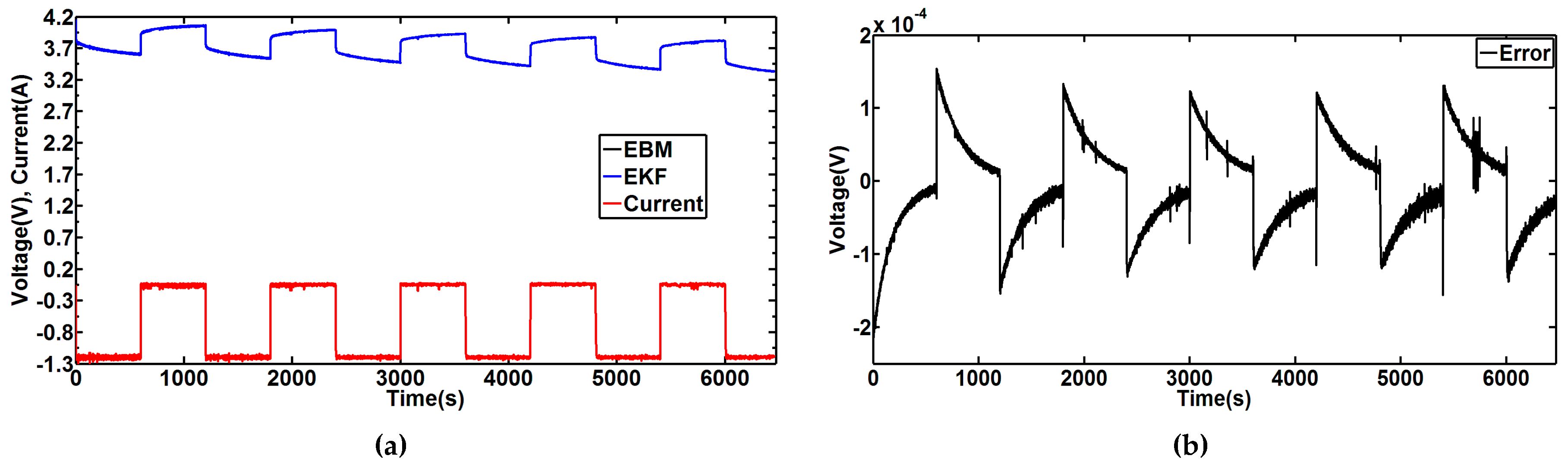
Firstly, we compared the voltage estimated by the EKF with the voltage output of the EBM model, based on the same current. The battery is discharged with a current of 1.2 A (600 s on-time and 600 s off-time) as shown in Figure 12a. This Figure shows the voltages obtained with EKF and EBM. The voltage error is lower than 0.02% as shown in Figure 12b.

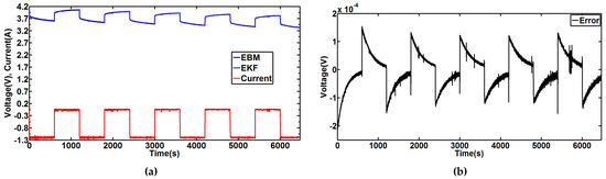
Figure 12. Extended battery model (EBM) and extended Kalman filter (EKF) voltages for 1.2 A current profile (a) voltages and current, (b) voltage error.

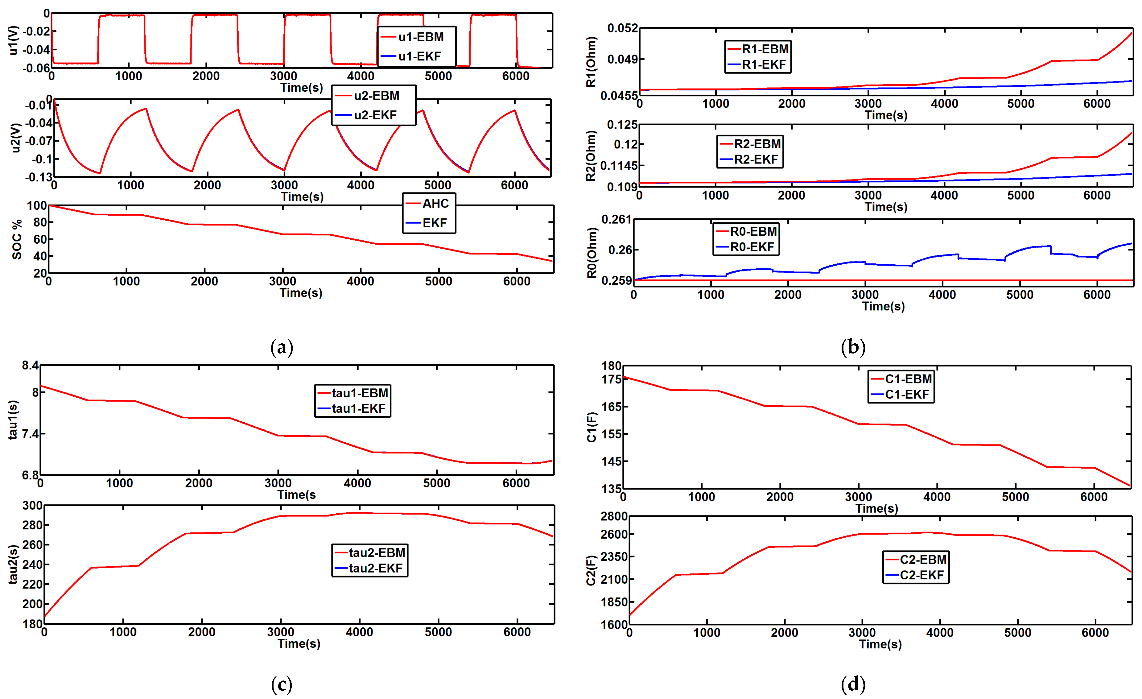
Figure 13 compares the battery parameters for the EBM with the EKF-estimated parameters ($u_1$, $u_2, \mathrm{SOC}$, ${\tau }_1$, $C_1$, ${\tau }_2$, $C_2, R_1, R_2$ and $R_0$). It is observed that the estimator can accurately identify the battery parameters of the model. For Figure 13a,c,d, the output curves obtained with EKF and EBM are virtually identical and so are superimposed in the graphs.

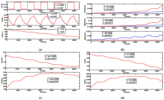
Figure 13. Comparison of EBM and EKF results for the 1.2 A current profile (a) plot of $u_1$, $u_2$ and $\mathrm{SOC}$, (b) resistances $R_1,R_2$ and $R_0$ (c) time constants ${\tau }_1$ and ${\tau }_2$ (d) capacitances $C_1$ and $C_2$.

These estimated parameters vary with time due to their variation with $\mathrm{SOC}$. The main observations concern the resistances which do not vary significantly with time. There is some fluctuation in resistance $R_0$, but it seems to be low.

These resistances vary slightly for a $\mathrm{SOC}$ interval of 30–100%; conversely, capacitances vary considerably with $\mathrm{SOC}$. These hypothetical observations can be confirmed by experimental results.

9.2. Validation using Experimental Signals

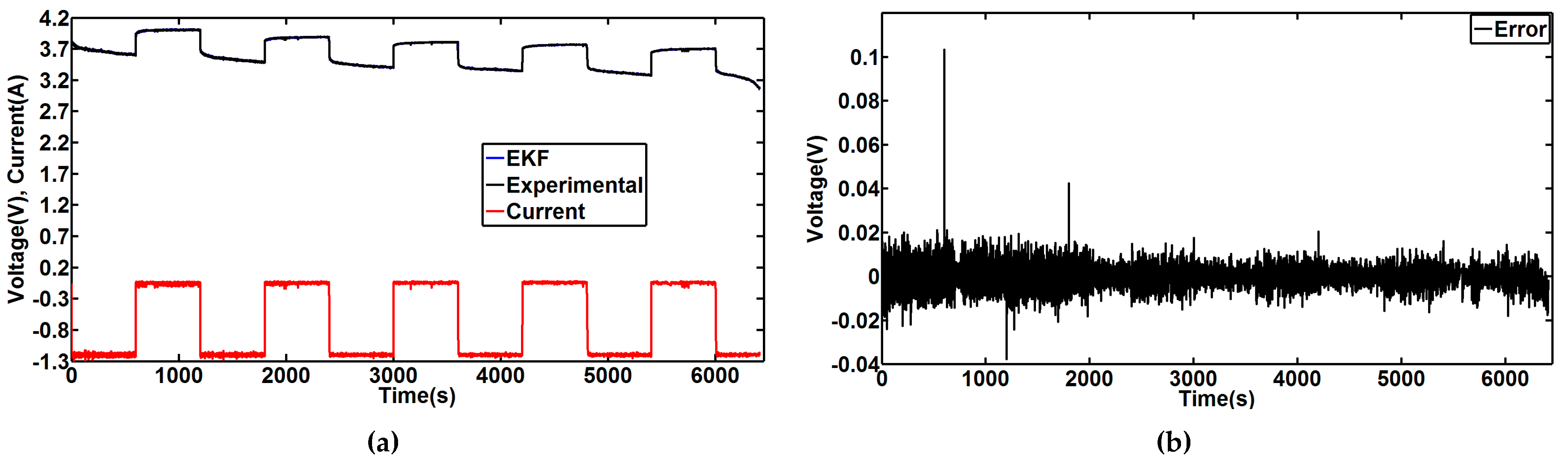
To validate the EKF observer, we used the same current profile shown previously in Figure 12a. The battery voltage over time was measured experimentally and compared with the voltage estimated by the CD-EKF estimator. As seen in Figure 14, the voltage with CD-EKF converges with the experimental data, and the error between these voltages is very low (on the order of 2 mV).

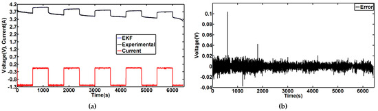
Figure 14. Experimental and EKF voltages for the 1.2 A current profile (a) voltages and current, (b) voltage error.

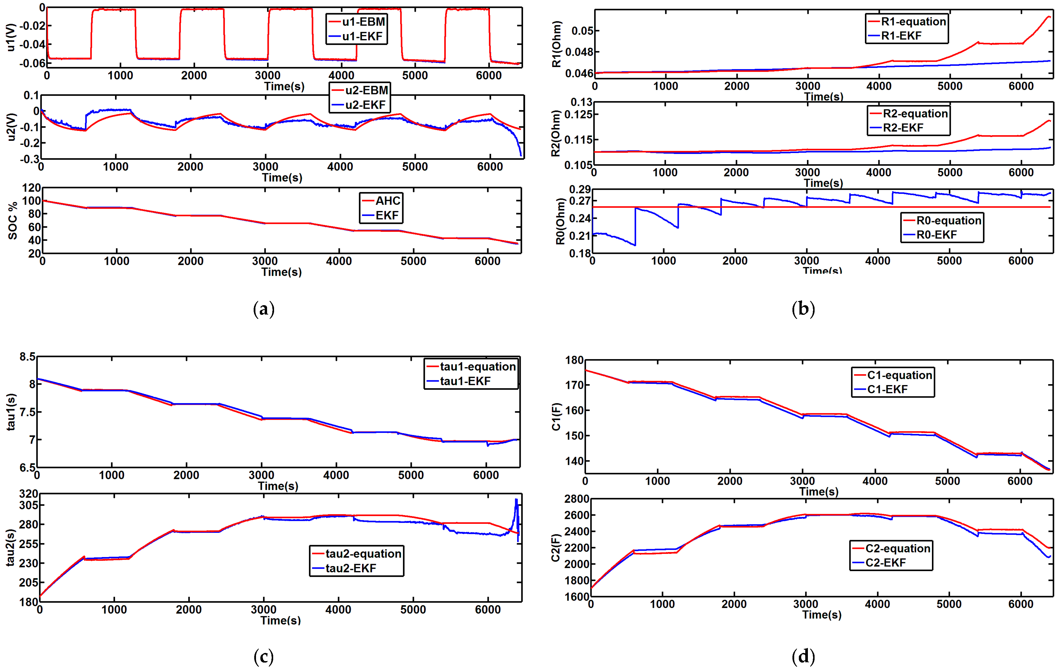
Figure 15 shows the variation of parameters with time. The parameters of the EKF estimator are initialized with values slightly different from the true ones. The estimated drop voltages $u_1$ and $u_2$ are compared with values obtained using the EBM, as presented in Figure 15a. The first voltage drop is close to the value obtained with the EBM, but the voltage drop $u_2$ is greater than $u_1$, yet it can be influenced by different coefficients, such as temperature. This can lead to errors determining the concentration parameters ($R_2$ and $C_2$), particularly at the beginning of discharge.

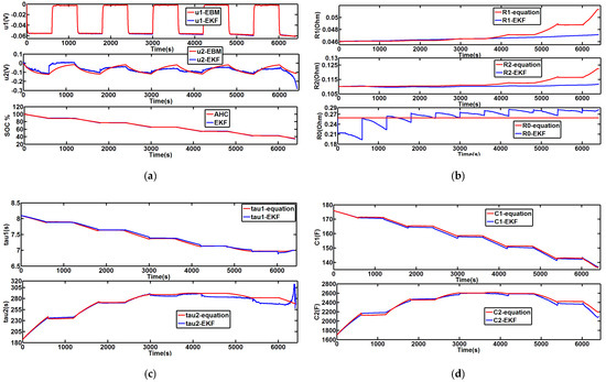
Figure 15. EKF results for 1.2 A current profile (a) plot of $u_1$, $u_2$ and $\mathrm{SOC}$, (b) resistances $R_1,R_2$ and $R_0$ (c) time constants ${\tau }_1$ and ${\tau }_2$ (d) capacitances $C_1$ and $C_2$.

The values for resistance and the capacitance estimated by CD-EKF are compared with those calculated by theoretical Equations (9) and (10) using the $\mathrm{SOC}$ value obtained by the estimator. These results are shown in Figure 15a–d. The temporal change of the estimated parameters matches the calculations closely.

The main difficulties when determining these parameters usually reside at the beginning and the end of discharge. For this CD-EKF estimator, minor errors occur, especially at low $\mathrm{SOC}$. It is found that the relative error of the estimated parameters oscillates around the zero value. Maximum error is presented in Table 2.

Table 2. Maximum relative errors of estimated parameters.

Parameter	Error
$\mathsf{\Delta }{\tau }_1$	$1\%$
$\mathsf{\Delta }{C}_1$	$0.9\%$
$\mathsf{\Delta }{\tau }_2$	$5\%$
$\mathsf{\Delta }{C}_2$	$4\%$
$\mathsf{\Delta }{R}_1$	$5\%$
$\mathsf{\Delta }{R}_2$	$6\%$
$\mathsf{\Delta }{R}_0$	$8\%$

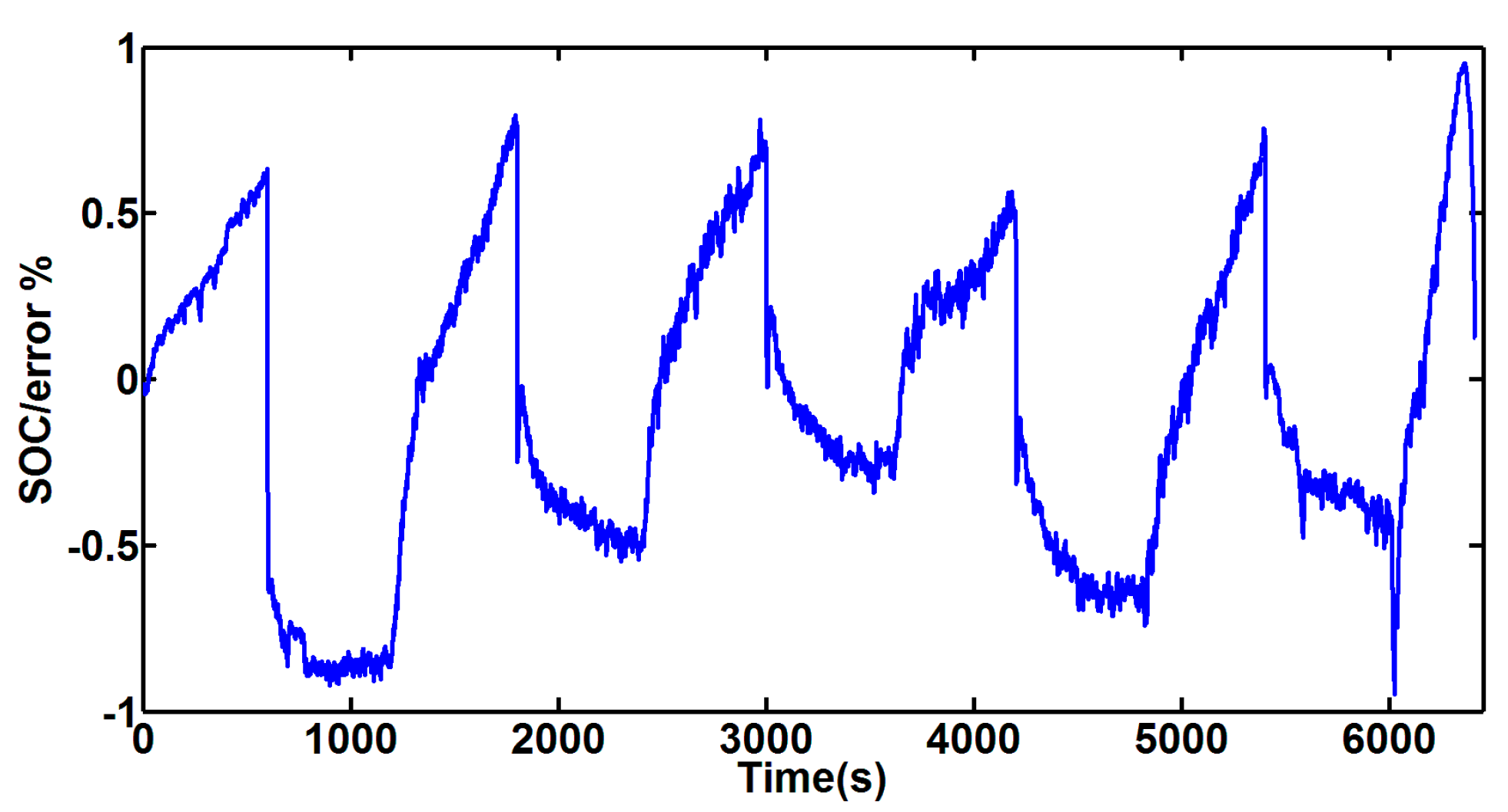
The $\mathrm{SOC}$ results estimated with EKF and AHC are compared in Figure 15a. The $\mathrm{SOC}$ with EKF converges to the value with AHC with error lower than 1% as shown in Figure 16.

Figure 16. $\mathrm{SOC}$ estimation error.

10. Conclusions

In this paper, we propose an extended model to simplify the characterisation of battery parameters (state of charge, resistances and capacitances). This lithium-ion battery model relies on iterative measures of voltage and current as well as estimations from a continuous-discrete extended Kalman filter. We employed the pulse discharge method and fitting technique to determine battery parameters and to validate the model experimentally.

The model, established in the MATLAB environment, takes into account the effect of the discharge rate on battery parameters, and simulates the dynamic voltage behaviours of the battery well. It satisfies a trade-off between complexity and precision. However, at the end of discharge, the model becomes less precise because of increasing superposed errors and electrochemical phenomena that may take place at low voltage. For more stable estimates of the state of charge, further research can be performed to determine the time constants.

Although the model adjusts for Coulombic efficiency variation, temperature can have a substantial effect on battery behaviour and needs to be analysed more deeply.

We have developed a CD-EKF estimator based on the battery model we first derived, using an EKF observer to update parameters for ongoing, iterative input to the model. One of the great advantages of using the observer is the ability to recover from incorrect initial conditions.

Experimental results indicate that this revised CD-EKF estimator can accurately determine battery parameters throughout most of the discharge cycle. In further study, we are currently working to apply the developed estimator in real time measurements with another battery.

The estimator uses only a few equations, and should not require significant computing resources. The developed estimator can be used in various applications such as laptops, telephones and electric vehicles. We are also considering using extended Kalman filters to create an online tool for estimating the state of health of batteries online.

References

- Andre, D.; Meiler, M.; Steiner, K.; Wimmer, C.; Soczka-Guth, T.; Sauer, D.U. Characterization of high-power lithium-ion batteries by electrochemical impedance spectroscopy. I: Experimental investigation. J. Power Sources 2011, 196, 5334–5341. [Google Scholar] [CrossRef]
- Andre, D.; Meiler, M.; Steiner, K.; Walz, H.; Soczka-Guth, T.; Sauer, D.U. Characterization of high-power lithium-ion batteries by electrochemical impedance spectroscopy. II: Modelling. J. Power Sources 2011, 196, 5349–5356. [Google Scholar] [CrossRef]
- Smith, K.A.; Rahn, C.D.; Wang, C.-Y. Model-based electrochemical estimation and constraint management for pulse operation of lithium ion batteries. IEEE Trans. Control Syst. Technol. 2010, 18, 654–663. [Google Scholar] [CrossRef]
- Bhangu, B.S.; Bentley, P.; Stone, D.A.; Bingham, C.M. Nonlinear observers for predicting state-of-charge and state-of-health of lead-acid batteries for hybrid-electric vehicles. IEEE Trans. Veh. Technol. 2005, 54, 783–794. [Google Scholar] [CrossRef]
- Subburaj, A.S.; Bayne, S.B. Analysis of dual polarization battery model for grid applications. In Proceedings of the IEEE 36th International Telecommunications Energy Conference (INTELEC), Vancouver, BC, Canada, 28 September–2 October 2014; pp. 1–7. [Google Scholar]
- Chen, M.; Rincon-Mora, G.A. Accurate electrical battery model capable of predicting runtime and IV performance. IEEE Trans. Energy Convers. 2006, 21, 504–511. [Google Scholar] [CrossRef]
- Piller, S.; Perrin, M.; Jossen, A. Methods for state-of-charge determination and their applications. J. Power Sources 2001, 96, 113–120. [Google Scholar] [CrossRef]
- Einhorn, M.; Conte, V.; Kral, C.; Fleig, J. Comparison of electrical battery models using a numerically optimized parameterization method. In Proceedings of the IEEE Vehicle Power and Propulsion Conference (VPPC), Chicago, IL, USA, 6–9 September 2011; pp. 1–7. [Google Scholar]
- Spotnitz, R. Simulation of capacity fade in lithium-ion batteries. J. Power Sources 2003, 113, 72–80. [Google Scholar] [CrossRef]
- Pop, V.; Bergveld, H.J.; Danilov, D.; Regtien, P.P.; Notten, P.H. Battery Management Systems: Accurate State-of-Charge Indication for Battery-Powered Applications; Springer Science & Business Media: Berlin, Germany, 2008. [Google Scholar]
- Xiong, R.; He, H.; Sun, F.; Zhao, K. Online estimation of peak power capability of Li-ion batteries in electric vehicles by a hardware-in-loop approach. Energies 2012, 5, 1455–1469. [Google Scholar] [CrossRef]
- Xiong, R.; Gong, X.; Mi, C.C.; Sun, F. A robust state-of-charge estimator for multiple types of lithium-ion batteries using adaptive extended Kalman filter. J. Power Sources 2013, 243, 805–816. [Google Scholar] [CrossRef]
- Hu, C.; Youn, B.D.; Chung, J. A multiscale framework with extended Kalman filter for lithium-ion battery SOC and capacity estimation. Appl. Energy 2012, 92, 694–704. [Google Scholar] [CrossRef]
- Chen, Z.; Qiu, S.; Masrur, M.A.; Murphey, Y.L. Battery state of charge estimation based on a combined model of Extended Kalman Filter and neural networks. In Proceedings of the 2011 International Joint Conference on Neural Networks (IJCNN), San Jose, CA, USA, 31 July–5 August 2011; pp. 2156–2163. [Google Scholar]
- Andre, D.; Nuhic, A.; Soczka-Guth, T.; Sauer, D.U. Comparative study of a structured neural network and an extended Kalman filter for state of health determination of lithium-ion batteries in hybrid electricvehicles. Eng. Appl. Artif. Intell. 2013, 26, 951–961. [Google Scholar] [CrossRef]
- Särkkä, S.; Sarmavuori, J. Gaussian filtering and smoothing for continuous-discrete dynamic systems. Signal Process. 2013, 93, 500–510. [Google Scholar] [CrossRef]
- Kulikov, G.Y.; Kulikova, M.V. High-order accurate continuous-discrete extended Kalman filter for chemical engineering. Eur. J. Control 2015, 21, 14–26. [Google Scholar] [CrossRef]
- Hua, Y.; Xu, M.; Li, M.; Ma, C.; Zhao, C. Estimation of state of charge for two types of Lithium-Ion batteries by nonlinear predictive filter for electric vehicles. Energies 2015, 8, 3556–3577. [Google Scholar] [CrossRef]
- Kim, T.; Qiao, W. A hybrid battery model capable of capturing dynamic circuit characteristics and nonlinear capacity effects. IEEE Trans. Energy Convers. 2011, 26, 1172–1180. [Google Scholar] [CrossRef]
- Nikolian, A.; Firouz, Y.; Gopalakrishnan, R.; Timmermans, J.M.; Omar, N.; van den Bossche, P.; van Mierlo, J. Lithium ion batteries—Development of advanced electrical equivalent circuit models for nickel manganese cobalt lithium-ion. Energies 2016, 9, 360. [Google Scholar] [CrossRef]
- He, H.; Zhang, X.; Xiong, R.; Xu, Y.; Guo, H. Online model-based estimation of state-of-charge and open-circuit voltage of lithium-ion batteries in electric vehicles. Energy 2012, 39, 310–318. [Google Scholar] [CrossRef]
- Panasonic DataSheet. Available online: http://www.alldatasheet.com/datasheet-pdf/pdf/219494/PANASONIC/CGR18650CF.html (accessed on 11 May 2017).
- He, H.; Xiong, R.; Fan, J. Evaluation of lithium-ion battery equivalent circuit models for state of charge estimation by an experimental approach. Energies 2011, 4, 582–598. [Google Scholar] [CrossRef]
- Feng, F.; Lu, R.; Zhu, C. A combined state of charge estimation method for lithium-ion batteries used in a wide ambient temperature range. Energies 2014, 7, 3004–3032. [Google Scholar] [CrossRef]
- Garche, J.; Dyer, C.K.; Moseley, P.T.; Ogumi, Z.; Rand, D.A.; Scrosati, B. Encyclopedia of Electrochemical Power Sources; Newnes: Sydney, Australia, 2013. [Google Scholar]
- Jiang, J.; Liu, Q.; Zhang, C.; Zhang, W. Evaluation of acceptable charging current of power Li-ion batteries based on polarization characteristics. IEEE Trans. Ind. Electron. 2014, 61, 6844–6851. [Google Scholar] [CrossRef]
- Chun, C.Y.; Seo, G.-S.; Yoon, S.H.; Cho, B.-H. State-of-charge estimation for lithium-ion battery pack using reconstructed open-circuit-voltage curve. In Proceedings of the 2014 International Power Electronics Conference (IPEC-Hiroshima 2014-ECCE-ASIA), Hiroshima, Japan, 18–21 May 2014; pp. 2272–2276. [Google Scholar]
- Xu, J.; Mi, C.C.; Cao, B.; Deng, J.; Chen, Z.; Li, S. The state of charge estimation of lithium-ion batteries based on a proportional-integral observer. IEEE Trans. Veh. Technol. 2014, 63, 1614–1621. [Google Scholar]
- Yao, L.W.; Aziz, J.A. Modeling of Lithium Ion battery with nonlinear transfer resistance. In Proceedings of the IEEE Applied Power Electronics Colloquium (IAPEC), Johor Bahru, Malaysia, 18–19 April 2011; pp. 104–109. [Google Scholar]
- Kim, J.H.; Lee, S.J.; Kim, E.S.; Kim, S.K.; Kim, C.H.; Prikler, L. Modeling of battery for EV using EMTP/ATP draw. J. Electr. Eng. Technol. 2014, 9, 98–105. [Google Scholar] [CrossRef]
- Diab, Y.; AbouKair, M. Electric Energy Storage; Damascus University: Damascus, Syria, 2014; pp. 131–133. [Google Scholar]
- Kim, J.; Shin, J.; Chun, C.; Cho, B.H. Stable configuration of a Li-ion series battery pack based on a screening process for improved voltage/SOC balancing. IEEE Trans. Power Electron. 2012, 27, 411–424. [Google Scholar] [CrossRef]
- Charkhgard, M.; Zarif, M.H. Design of adaptive H∞ filter for implementing on state-of-charge estimation based on battery state-of-charge-varying modelling. IET Power Electron. 2015, 8, 1825–1833. [Google Scholar] [CrossRef]
- Xiong, R.; He, H.; Sun, F.; Zhao, K. Evaluation on state of charge estimation of batteries with adaptive extended Kalman filter by experiment approach. IEEE Trans. Veh. Technol. 2013, 62, 108–117. [Google Scholar] [CrossRef]
- He, H.; Xiong, R.; Zhang, X.; Sun, F.; Fan, J. State-of-charge estimation of the lithium-ion battery using an adaptive extended Kalman filter based on an improved Thevenin model. IEEE Trans. Veh. Technol. 2011, 60, 1461–1469. [Google Scholar]
- Zhang, C.P.; Liu, J.Z.; Sharkh, S.M.; Zhang, C.N. Identification of Dynamic Model Parameters for Lithium-Ion Batteries used in Hybrid Electric Vehicles. Available online: https://eprints.soton.ac.uk/73265/1/Identification_of_Dynamic_Model_Parameters_for.pdf (accessed on 24 July 2017).
- Kulikov, G.Y.; Kulikova, M.V. Accurate numerical implementation of the continuous-discrete extended Kalman filter. IEEE Trans. Autom. Control 2014, 59, 273–279. [Google Scholar] [CrossRef]
- Axelsson, P.; Gustafsson, F. Discrete-time solutions to the continuous-time differential Lyapunov equation with applications to Kalman filtering. IEEE Trans. Autom. Control 2015, 60, 632–643. [Google Scholar] [CrossRef]
- Auger, F.; Hilairet, M.; Guerrero, J.M.; Monmasson, E.; Orlowska-Kowalska, T.; Katsura, S. Industrial applications of the Kalman filter: A review. IEEE Trans. Ind. Electron. 2013, 60, 5458–5471. [Google Scholar] [CrossRef]
© 2017 by the authors. Licensee MDPI, Basel, Switzerland. This article is an open access article distributed under the terms and conditions of the Creative Commons Attribution (CC BY) license (http://creativecommons.org/licenses/by/4.0/).