1. Introduction
Wind turbines are being increasingly integrated into weak grids that possess limited synchronous generators (i.e., are inertia weak) or long transmission lines (i.e., are link weak), a situation found in many areas in China [
1]. The impact of this large-scale integration of wind turbines on power system stability in such systems has been widely studied in terms of transient stability [
2,
3,
4,
5], small signal stability [
6,
7], and frequency stability [
8]. Based on these studies, many optimizations or re-designs of wind turbine controllers have been proposed to improve different aspects of power system stability [
9,
10,
11,
12,
13,
14,
15,
16].
In terms of transient stability, Ullah et al. [
11] proposed an E.ON-grid-code-compliant current reference controller that preferentially boosted the reactive current in proportion to the voltage dip to simultaneously support the system voltage and improve transient stability. A study by Weise [
12] further revealed there was a beneficial effect of the accompanied active current reduction with this type of controller on transient stability, and discussed the optimum setting of the proportional gain for reactive current boosting. Furthermore, [
13] proposed an independent active current reduction controller that optimized the active current reference with a multiplier approximately proportional to the square of the remaining voltage. In addition, [
14] proposed a torque reference controller that optimized the torque reference based on the terminal frequency for a rigid interval subsequent to a fault. Reference [
15] proposed a swing-equation-based constant-virtual-inertia control of wind turbines (virtual synchronous generators), and suggested a large constant virtual inertia setting for transient stability improvement. Comparatively, Alipoor et al. [
16] proposed a mutative virtual inertia controller, wherein each swing cycle of the virtual synchronous generator was divided into four stages, and the virtual inertia was set to be large for stages 1 and 3 and small for stages 2 and 4. A considerable improvement in transient stability was reported in the study.
Although numerous controllers have been proposed, and many associated problems have also been analyzed in the studies reviewed above, there are still two issues that have not received much attention. The first problem is the mechanism underlying transient stability improvement within a single (synchronous) machine infinite bus (SMIB) system. An analysis of this mechanism for simple SMIB systems can produce engineering insights that can be used to guide the design of the main structure of a controller for transient stability improvement in systems that are more complex. Another problem is how the capability of the active and reactive currents of a wind turbine are dependent on various physical factors—such as the location of the wind turbines and the strength of the grid—in terms of affecting the swing dynamics of synchronous machines. An analysis of the dependencies for simple systems can produce engineering insights that can be used to guide selection of the control object within a wind turbine’s active current and reactive current, as well as help recognition of the influential physical factors that must be considered in the parameter setting process for complex systems.
This paper first analyzes these two associated problems for very simple systems. The engineering insights gained are then used to design a wind turbine active current reference controller and its settings optimization in order to improve power system transient stability when large-scale wind turbines are integrated into weak grids. Finally, the paper will present an application of the proposed controller and its setting approach using Kundur’s two-area system modified by wind turbine integration.
The rest of this paper is organized as follows.
Section 2 and
Section 3 present analyses of the two problems, respectively.
Section 4 introduces the proposed controller and its settings approach.
Section 5 provides the case study using Kundur’s two-area system, while
Section 6 concludes the paper.
2. Analysis of the Mechanism for Transient Stability Improvement in Single Machine Infinite Bus (SMIB) Systems
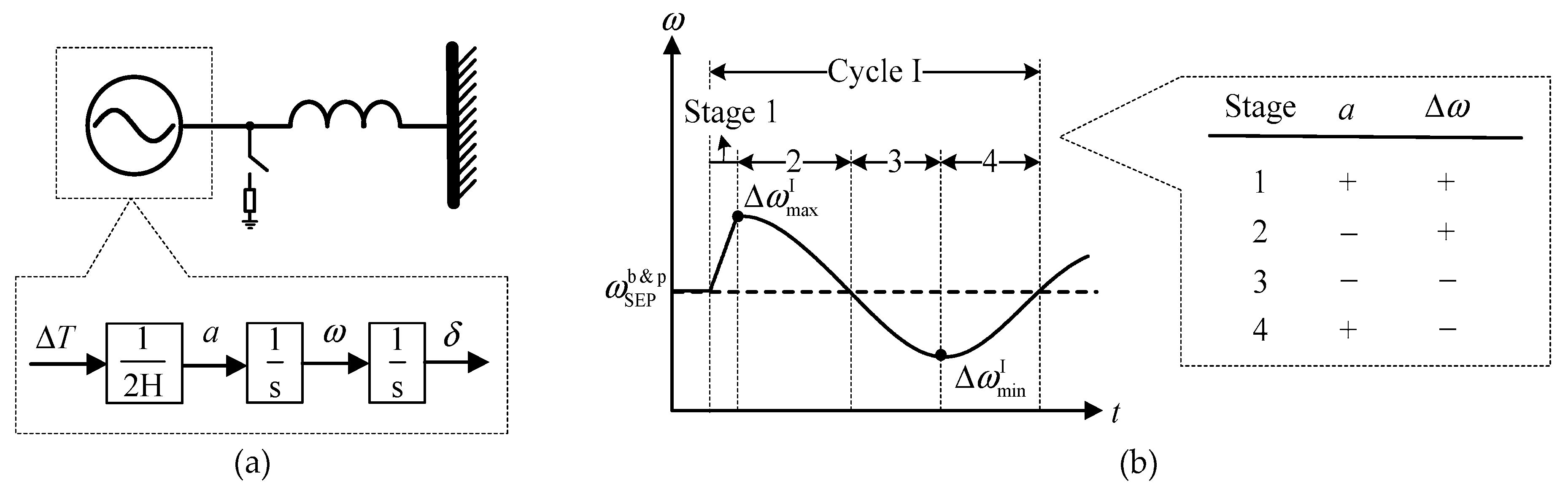
Using the stage division criterion developed by Alipoor et al. [
16], we reevaluate the mechanism providing transient stability improvement in an SMIB system. As illustrated in
Figure 1b, Alipoor et al. divided each swing cycle of the SMIB system shown in
Figure 1a into four stages. The interval with a positive rotor acceleration and a positive rotor speed deviation from its post-fault stable equivalent point (SEP) (assumed to be 1 p.u.) is stage 1; the interval with a negative rotor acceleration and a positive rotor speed deviation is stage 2, the interval with negative acceleration and negative speed deviation is stage 3, and the interval with positive acceleration and negative speed deviation is stage 4.
2.1. Quantitative Relationship between the Motivating Equivalent Rotor Acceleration of Each Stage and the Resulting Extrema of Rotor Speed and Angle Deviation from the Respective Post-Fault SEP Value
The transient stability of a SMIB system is, in fact, the stability of two variables, the rotor speed and rotor angle; both are essentially motivated by the rotor acceleration, as
Figure 1a exhibits. By using a constant rotor acceleration that equals the true time-varying acceleration in each stage, the quantitative relationship between rotor acceleration, rotor speed deviation, and rotor angle deviation during each stage can be written as
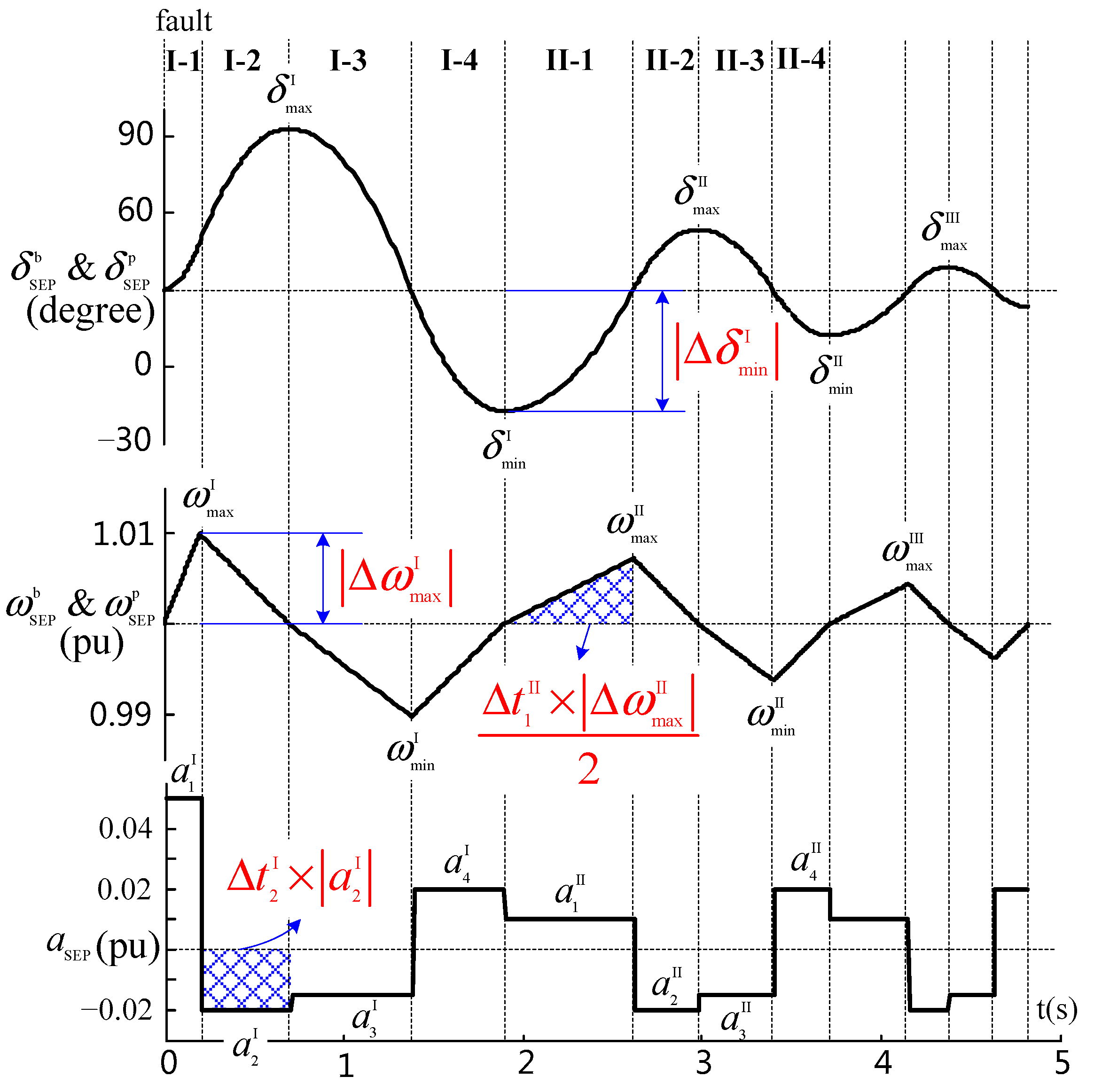
Figure 2 illustrates the typical swing process of a SMIB system, where the synchronous machine is accelerating during a fault and its rotor angle has passed the post-fault SEP value at fault clearance. The rotor acceleration is deliberately set to be constant during each stage, respectively denoted as
,
,
…
By repeatedly applying (1), the quantitative relationships between the motivating accelerations and the resulting extrema in speed and angle deviations for different swing processes of the SMIB system can be obtained. The expressions are slightly different depending on whether the synchronous machine is accelerating or decelerating during fault and whether or not the rotor angle has passed its post-fault SEP value at fault clearance; the expressions are presented in a dense form as follows.
The extrema of the deviations in rotor angle and speed from their respective SEP value in the first cycle, reflecting the first and second swing stabilities, are given by
where the “,” in subscript means “or”, with the former representing the situation when the synchronous machine accelerates during fault and the latter decelerates, the Arabic numerals in subscript are the stage number, the Roman numerals in superscript are the cycle number, the “clr” in subscript means fault clearance, the “Passed” in (2) and (4) represents the situation when the rotor angle has passed the post-fault SEP value at fault clearance and the “Not passed” represents the situation when the rotor angle has not passed. Furthermore,
where the superscript “p” represents “post fault”, and “b” represents “before fault”.
The extrema and their decays in subsequent cycles reflect aperiodic and oscillatory stabilities after the first cycle, and can be deduced as follows
with the exception that
if the rotor angle has passed its post-fault SEP value at fault clearance. The stage accelerations without cycle identifications in the right side of (9) and (10) are those between the two compared extrema.
We can deduce from (2)–(5) and (9)–(11) that the transient stability of the SMIB system, including the first and second swing stabilities in the first cycle and the aperiodic and oscillatory stabilities in the following cycles, can be uniformly improved by decreasing the magnitudes of the rotor accelerations in stages 1 and 3 and increasing the magnitudes of the rotor accelerations in stages 2 and 4 as much as possible.
2.2. Qualitative Analysis of the Destruction of Stage Sequence due to Improper Control Actions
The relationships obtained above are implicitly assumed to be a natural sequence, i.e., 1-2-3-4-1-2…, where each stage follows the same previous stage in their natural order. However, this natural sequence can be destroyed by improper controller actions, and significantly affecting power system transient stability.
Figure 3 sketches the segments of the electric power versus rotor angle
Pe-
δ relationship of a synchronous machine in a SMIB system that has been distorted by control actions. The blue segments show a natural stage sequence in one cycle where the stage cycle is 2-3-4-1. The red segments illustrate two cases of the destruction of the natural sequence, which will be analyzed below.
2.2.1. Destruction at Transition from Stage 2 to Stage 3
For a natural transition shown by the blue segments in the right part of
Figure 3, the control action in stage 3 should continue decelerating the synchronous generator. Such an action would lead to a negative speed deviation that decreases the accumulated positive angle deviation, but should use a smaller rotor acceleration to reduce the speed deviation that accompanies the process, as illustrated in
Figure 2. However, an excessive control action in stage 3, shown by the red segment 3′ in
Figure 3, will accelerate the synchronous machine, quickly resulting in a positive speed deviation. The system thus enters into stage 1 after a negligible stay in stage 3; the natural evolution sequence is destroyed and the rotor angle continues to increase. It is very likely that the rotor angle will increase beyond the unstable equivalent point (UEP) and causing an aperiodic instability for the following two reasons. First, the intrinsic
Pe-
δ characteristic (sine function) tends to reduce the electric power under these circumstances, resulting in a longer stay in stage 1 and a larger consequent angle deviation (i.e., moving further right in the
Pe-
δ plane). Secondly, the distance to the right UEP is already quite short at the end of stage 2.
2.2.2. Destruction at Transition from Stage 4 to Stage 1
A similar destruction can occur at the transition from stage 4 to stage 1 if the control action in stage 1 is excessive. The system will evolve back to stage 3 from stage 4 after a negligible stay in stage 1, as illustrated by the red segments 1′′ and 3′′ in the left part of
Figure 3. The consequence, however, is much less severe. The angle deviation becomes larger (i.e., moving further left in the
Pe-
δ plane), but an instability is not likely to happen for the following two reasons. First, the intrinsic
Pe-
δ characteristic tends to reduce the electric power under such circumstances, thus counteracting the control action in stage 3 and tending to pull the system back to the natural stage sequence. Secondly, the distance to the left UEP at the end of stage 4 is quite far.
The destructions above are both caused by an excessive control action in stage 1 or stage 3. Therefore, these destructions can be avoided by designing more moderate control actions for these two stages.
2.3. Mechanism of Transient Stability Improvement in a SMIB System
After combining the analyses in
Section 2.1 and
Section 2.2, we can hypothesize that the power system transient stability of a SMIB system—including the first and second swing stabilities in the first cycle and the aperiodic and oscillatory stabilities in the following cycles—can be uniformly improved by dramatically increasing the magnitudes of the rotor accelerations in stages 2 and 4 and by moderately decreasing the magnitudes of the rotor accelerations in stages 1 and 3.
3. Analysis of the Physical Factors Influencing the Capability of Wind Turbine Active and Reactive Currents to Affect the Swing Dynamics of Synchronous Machines
The physical factor dependencies are analyzed for a system with two synchronous machines and one aggregated wind turbine, shown in
Figure 4a, which experiences a three-phase fault cleared by isolation. The synchronous machines are represented by the classic model and the wind turbine is represented by a controllable current source. The resistance and susceptance of the devices in
Figure 4a are all neglected. The resulting equivalent circuits during (
Figure 4b) and post fault are arranged into concise forms exhibited in
Figure 4c,d.
For this system, we use the following simplifications
where the superscript “d” represents “during fault”, and the physical meanings of the undeclared variables can be deduced from
Figure 4c,d.
3.1. Quantification of the Dependencies
Quantifying precisely how the capability of a wind turbine’s active and reactive currents to affect the swing dynamics of synchronous machines is dependent on various physical factors is done in three steps: first quantifying the capabilities, then quantifying the physical factors, and finally determining the dependencies.
First, since rotor acceleration is the intrinsic motivating force of the swing dynamics as discussed in
Section 2.1, the capability to affect the swing dynamics can be quantified in terms of the rotor acceleration, given by
where Δ here represents a small change, different from those in (1)–(11),
a12 is the relative rotor acceleration between the two machines in
Figure 4 and represents the rotor acceleration of the equivalent SMIB system, and
and
represent the capability of the reactive and active current, respectively, to affect the swing dynamics of the synchronous machines. Furthermore, the magnitudes of
and
reflect the efficiency of optimizing the reactive and active currents, respectively, and their signs in combination with the stage status (i.e., which stage the swing process is in) determine the optimization direction (i.e., to increase or decrease), according to
Section 2.3. The resulting expressions of
and
are constructed from the variables in
Figure 4c,d.
Secondly, the physical factors are quantified using the variables in
Figure 4c,d. The system strength in terms of inertia and link impedance are respectively quantified as
and the system topology in terms of wind farm location and synchronous-generator (inertia-) distribution are respectively quantified as
The fault and its location is quantified by
where an infinite value of
γ represents clearance of the fault, and the physical meaning of the undeclared variables in (15)–(19) can be deduced from
Figure 4. In addition, the pre-fault power flow and other factors that mainly influence the range of rotor angle
δg12 during swings are quantified by the rotor angle
δg12. The physical characteristics of the wind turbines themselves are quantified by their active and reactive current injections
and
.
Third, we substitute the quantified physical factors into the original expressions of
and
, which gives
where
Equations (20) and (21) link the quantified capabilities and the quantified physical factors. Consequently, the dependence of the capabilities on one physical factor can be quantified as the impact of the corresponding variable of this physical factor on the magnitudes and signs of and , respectively, given by (20) and (21). In other words, any analysis of the dependencies is changed into an analysis of (20) and (21), which means mathematical tools such as function curves and partial derivatives can now be employed in the analysis.
3.2. Analysis of the Dependencies
This analysis is divided into two parts. The first part provides a general but basic analysis, covering various physical factors. The second part provides an in-depth but specific analysis, focusing on the physical factor of wind turbine active current injection.
3.2.1. A General Basic Analysis
This part will analyze the general differences and similarities between the capability dependencies of a wind turbine’s active current and those of the reactive current.
We can deduce from (20) and (21) that the magnitudes of and both increase with a decrease in total inertia H, an increase in the inertia-distribution imbalance , or an increase in γ. Furthermore, we can also find that and always appear with X in a form of and , respectively. Combining these deductions with physical meanings of the variables gives the following similarities. Optimizations of the reactive and active current in terms of transient stability improvement are both more effective for inertia-weak grids (i.e., grids with limited synchronous generators) or severely unbalanced synchronous-generator-distribution grids. Additionally, they are both less effective during faults, especially when faults are close to the wind turbine. Besides, a link-weak grid (i.e., a grid with long transmission lines) magnifies both impacts of wind turbine active and reactive currents on the performance of their optimizations.
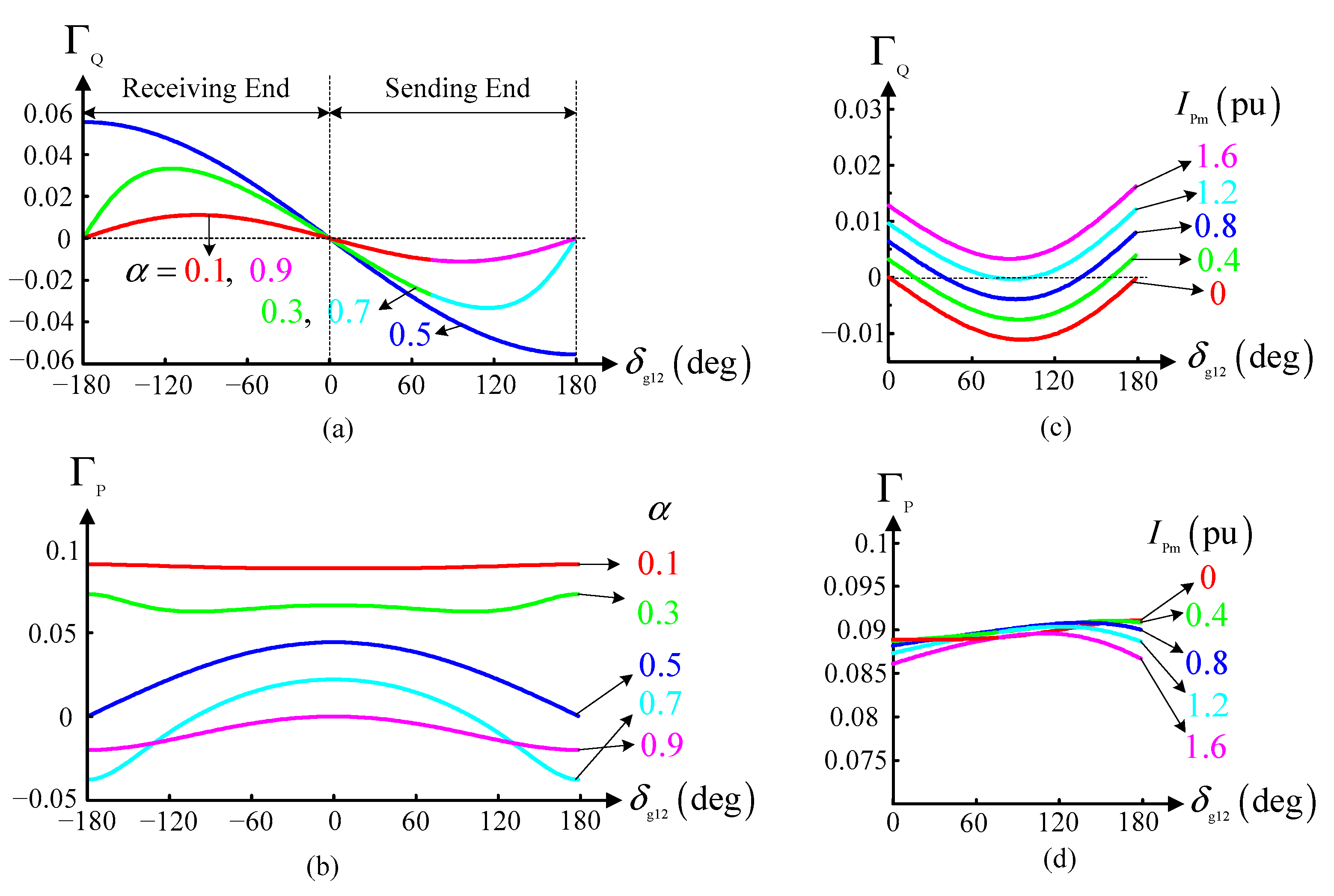
Figure 5 offers curves of
and
with different parameter values. We can see from
Figure 5a,b that the magnitude of
decreases as
increases, while the magnitude of
, to some extent, increases as
increases. We can also find that
is always heavily affected by the rotor angle
δg12, while
is barely affected by
δg12 when its magnitude is large. Combining these deductions with the physical meanings of the variables shows certain differences. Optimization of the reactive current is more effective when a wind farm is located near the middle of the transmission lines, and is less effective when placed near the ends. In comparison, optimization of the active current is less effective near the middle and more effective near the ends, i.e., complementary to the reactive current. The performance of any reactive current optimization is always heavily affected by any physical factors that heavily influence the rotor angle range during swings, such as pre-fault power flow. In comparison, any effects on active current are negligible when its optimization is considerably effective, e.g., when the wind farm is located at the end of a long transmission line and there are limited synchronous generators nearby (i.e., the wind farm integrates into a weak grid).
The analysis above identifies the general physical factors that may need to be considered during the parameter setting process of the controller. Some of these factors are deterministic, such as the system strength and the wind farm location, and can be handled offline. However, others are not deterministic—or are stochastic like the pre-fault power flow and fault location—and may need online adaptation.
3.2.2. An In-Depth Specific Analysis
This section focuses on the physical factor of the active current injection of wind turbines, the most significant difference between wind turbines and power electronic var-compensation devices such as static var compensators (SVCs), which possess many similar characteristics to wind turbines and have been well studied [
17,
18]. Since the effect of
on
and
, as suggested in (20)–(21), is quite complex and highly dependent on other variables such as
α and
β, the analysis is restricted to the following condition restrictions: a small
α, a small
β, a large
, and a positive
δg12. These conditions represent the scenario for which the proposed controller is designed, i.e., large-scale wind turbines integrate into weak grids.
The curves of
and
under the above conditions and with different active current injection levels (different
) are illustrated in
Figure 5c,d. First, the figures illustrate that the magnitude of
is always much larger than that of
, indicating that optimizing the active current is more effective than optimizing the reactive current under the given scenarios. This conclusion agrees with the general analysis in terms of wind farm location described in
Section 3.2.1.
Secondly, we can see from
Figure 5c,d that the curves of
are highly distorted by
, while the distortion for
is negligible. When
equals zero, as in the case of var-compensation devices, the sign of
is completely negative. Combining this result with the analysis in
Section 2.3 gives the conclusion that boosting the reactive current during the first swing is beneficial for first swing stability improvement, and that further optimization of reactive current post the first swing for further stability improvement only needs the information of stage status and thus is easy to implement. When
increases to a large non-zero value (technically,
increases to a large non-zero value, see the similarities in
Section 3.2.1), as in the case of wind turbines, the sign of
becomes partially negative or completely positive. Combining this with
Section 2.3 suggests that the beneficial effects of reactive current boosting are weakened or can even become detrimental, and that a high-efficiency controller of reactive current during or post the first swing now needs extra information concerning the sign of
. However, as shown in
Figure 5c, this sign further depends on rotor angle
δg12, a variable hard to estimate both offline and online. Therefore, a large-scale active current injection weakens or even reverses the beneficial impacts of reactive current boosting during the first swing, and makes the implementation of a high-efficiency controller of reactive current extremely difficult.
The high resistance of
to
, shown in
Figure 5d, eliminates the adverse impacts similar to those in the case of
. An always positive
, in combination with the analysis in
Section 2.3, suggests that a reduction in active current during the first swing is always beneficial for first swing stability improvement, and that further optimization of active current after the first swing for further stability improvement simply needs the information of stage status, regardless of the active current injection level. Therefore, a high-efficiency active current controller is easier to implement, under the given scenarios, than a similar reactive current controller, since it does not need any extra information that is hard to acquire, such as the rotor angle
δg12.
The above analysis shows the superiority of using active current over reactive current as the control object to improve the transient stability of weak grids with large-scale integrations of wind turbines. That is, the optimization of active current is more effective, and is easier to implement under these situations. Furthermore, the optimization of active current is also more flexible, as reactive current optimization is highly restricted by voltage supporting and regulating requirements.
Note that the same conclusions as those drawn from the qualitative analysis of the function curves of and in this section can also be drawn from a strict but lengthy mathematical analysis of the respective partial derivatives of and , which have not been presented here for the sake of brevity.
5. Applying the Proposed Controller and Its Settings Optimization to Kundur’s Two-Area System Modified with Wind Turbine Integration
An application of the proposed controller and the method for determining its settings to a test system is provided in this section. There are many common test systems for power system transient stability study such as WSCC 9-bus system, Kundur’s two-area system, New England system and Nordic32 system. We chose Kundur’s two-area system [
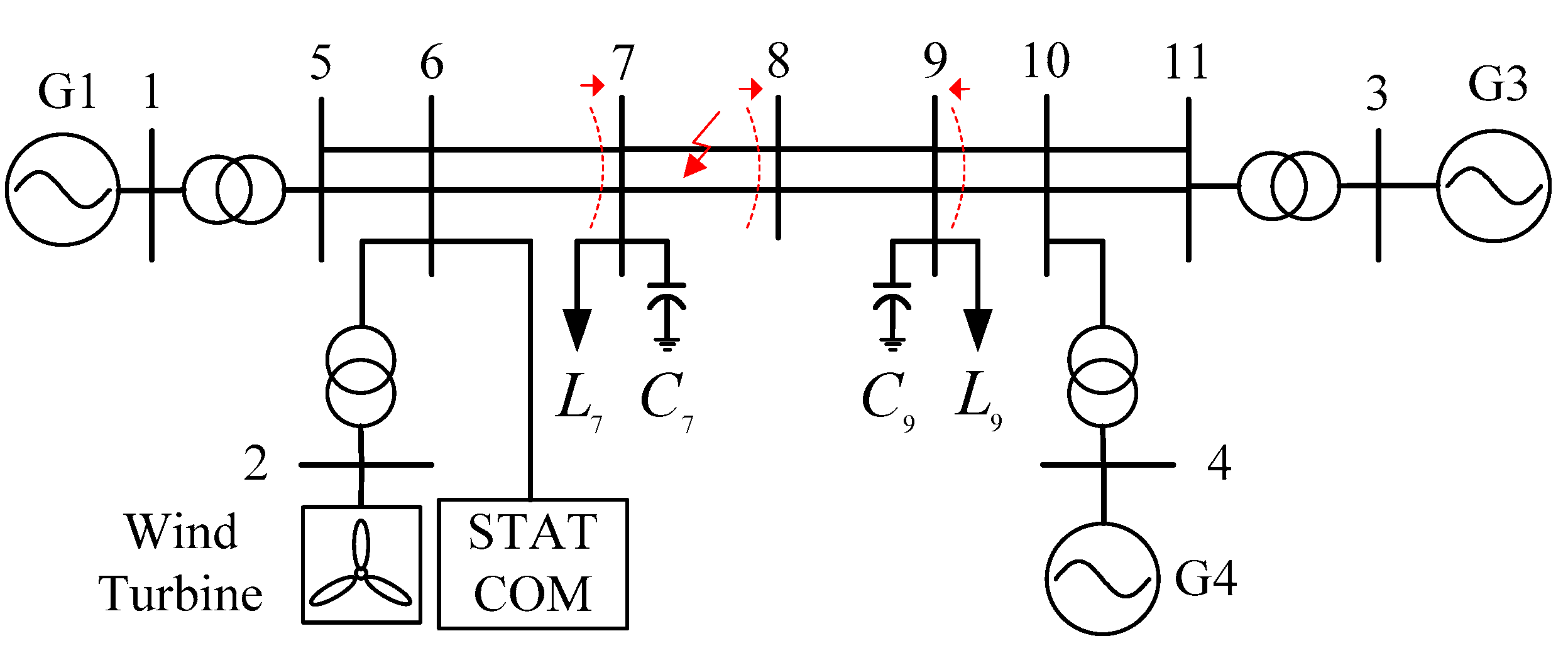
20], since it is a typical weak grid featured with long transmission lines and heave power flows. This test system was modified by replacing G2 with an equivalent wind farm (467 × 1.5 MW/1.67 MVA). The modification further weakened the strength of the system by reducing the inertia of the system. The wind farm was represented by an aggregated wind turbine. The pre-fault active power of G2 was balanced by the wind farm, and the reactive power was balanced by a STATCOM. Additionally, the transmission lines between bus 5–6, 6–7, 9–10 and 10–11 were doubled in both number and length (i.e., technically no change). The modified two-area system is shown in
Figure 7, and the information about the system strength and pre-fault power flow is provided in
Table 1.
Figure 7 also illustrates the measurement point of the corridor power in
Table 1 and the default fault location.
The model of the aggregated wind turbine was based on [
21]. The original supplementary controllers of current references preferentially boosted the reactive current and depressed the active current based on voltage dip. The structure of the original controllers, as well as their parameter settings, are presented in
Figure 8, which also demonstrates a way to incorporate the proposed controller. The models and parameter settings of other elements in the system are the same as those in [
20]. The fourth excitation control system in [
20] was used for the synchronous generators, i.e., a thyristor exciter with high gain and power system stabilizer.
For the parameter setting process of the proposed controller, we neglected the resistance and susceptance of the devices in
Figure 7, and all shunt-connected devices (excluding the wind turbines) along the transmission lines such as loads and capacitors. The fault set was chosen to be three-phase short-circuit faults on transmission line segments 7–8 and 8–9. The setting results are
In the simulation, the rotor acceleration/speed of the system’s equivalent SMIB system was estimated by the relative rotor acceleration/speed between G1 and G3, shown in
Figure 8. The resulting parameter settings are
where the time constant of the frequency measurement setting T
ωg is based on [
22], and the transmission delay setting
τ is from [
23].
The action of the proposed controller was limited to the first two cycles to avoid an increasingly detrimental effect of the delays of
Figure 8 in subsequent cycles. This is because the durations of the stages—particularly stages 2 and 4 as illustrated in
Figure 2—decrease with the damping of the swings, which increases the relative error in stage status caused by the delays and further deteriorates the efficiency of the controller.
The performance of the proposed controller and its settings optimization method were evaluated in three aspects, namely fault location, wind speed, and system strength. Multiple case pairs were designed for each aspect, and the only difference within each case pair was whether the proposed controller was incorporated into the wind turbine control or not. The resulting power system transient stability levels were assessed according to the critical clearing time (CCT), with a standard error of 10 ms. The CCT was determined by multiple time-domain simulations. The performance of the proposed controller under each case pair was thus quantified as the improvement in CCTs.
The proposed controller was first evaluated under different fault locations. Six case pairs were designed, representing a fault location at the middle of the transmission line segment 5–6, 6–7, 7–8, 8–9, 9–10, and 10–11, respectively. The fault was a three-phase short-circuit fault and was cleared by isolating the faulted line segment.
Table 2 shows the CCT results. The improvements (imp.) of the CCTs with (w/) the proposed controller, compared to those without (w/o) the proposed controller, suggest a high performance of the proposed controller under different fault locations.
The proposed controller was then evaluated under different wind speeds. Apart from the default wind speed of 11.5 m/s, four more wind speeds were considered as shown in
Table 3, which also exhibits the pre-fault active power output, rotor speed and pitch angle of the wind turbine under these wind speeds. The possible change in wind turbine active power output caused by the different wind speed was balanced by adjusting the active power outputs of the synchronous generators in proportion to their capacities. Therefore, the pre-fault power flow of the system might also be changed.
Table 3 presents the pre-fault corridor power flow near bus 8 under these wind speeds. For each case pair, the fault was located at the middle of the line segment 7–8, and the type and clearance of the fault as well as other settings were the same as above.
Table 4 presents the results. The improvements in CCTs verify the efficiency of the controller under different wind speeds.
Finally, the proposed controller was evaluated under different grid strengths. The strength of the test system in terms of link impedance was changed by proportionally adjusting the lengths of all transmission lines to 75% or 125% of their original values. The strength in terms of inertia was changed by proportionally adjusting the inertias of all synchronous generators to 75% or 125%. The parameter settings of the proposed controller were re-calculated, since some of the influential parameters recognized in
Section 3.2.1 had been changed.
Table 5 shows the controller settings and the short-circuit ratios (SCRs) at bus 2 (i.e., the SCR for the wind farm) under these grid strengths. The fault sequence and other settings remained unchanged.
Table 6 presents the CCT results. As can be found from
Table 6, the improvements in CCTs increase with the decrease of the system strength. In other words, the proposed controller performs better under weak grids. This finding conforms to the analysis of
Section 3.2.1, which states that the performance of active current optimization would be better under weak grids.
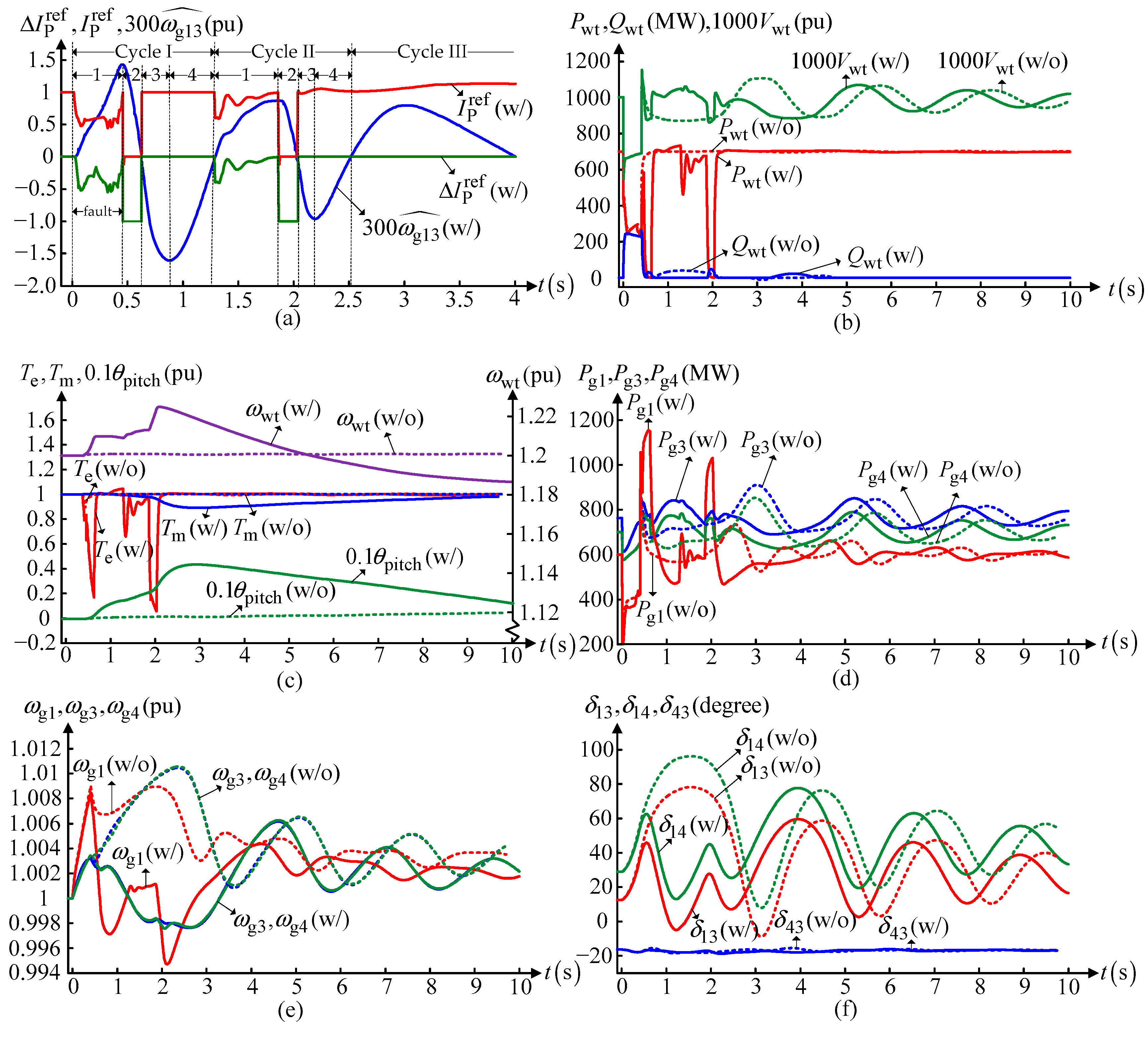
Time-domain dynamics of some variables within the case pair corresponding to 125% length of all transmission lines are provided in
Figure 9, with a fault duration of 410 ms.
Figure 9a shows the dynamics of the variables that reflect the action of the proposed controller. The mismatch between the corrective reference
and the final reference
during fault was due to the action of the current reference limit controller shown in
Figure 8. The 300
means 300 times of the
.
Figure 9b exhibits the active power, reactive power and terminal voltage of the aggregated wind turbine. The impact of the proposed controller on the rotor speed of the wind turbine is illustrated in
Figure 9c, which also presents the dynamics of other related variables including the pitch angle and the mechanical and electrical torques. The mismatch between the electric torque in
Figure 9c and the electric power in
Figure 9b was due to the action of the dynamic braking resistor that activates when the output power is much less than its order and causes an unacceptable DC-link voltage increase. The impacts on the synchronous generators are provided in
Figure 9d–f, demonstrating dynamics of active power outputs, rotor speeds, and relative rotor angles of/among synchronous generators, respectively.


