2.1. Requirements and Restrictions of Long-Haul Transportation
On German highways the long-haul freight transportation is mostly provided by semi-trailer trucks with a total weight of up to 40 t including the load weight [
14]. In general driving distances over 150 km are considered as long-haul transportation.
Figure 1 shows the number of long-haul trips for different distances within German inland freight transportation for years 2013 and 2014.
The trips cover a variety of distance levels, but about 69% of trips in 2014 have a distance of below 350 km. Assuming an average trip speed of 80 km/h truck drivers can drive these trips without a rest period. A rest period of at least 45 min is compulsory after 4.5 h driving according to the EU legislative regulation [
17]. The rest period can also be split into two rest periods of 15 min and 30 min and the shorter rest period can be shifted within the 4.5 h driving sequence. Subsequently to the longer rest period of 30 min or 45 min, the driver is allowed to drive an additional 4.5 h sequence. Afterwards the daily driving time maximum is reached and the nightly rest period follows. This driving time pattern is used in this study to define the transportation scenarios described in
Section 2.5. However, the German trucks account for only 20% of transportation performance within the transnational goods transport [
18] where long-haul routes are common. Hence foreign trucks also have to be considered, as done in this study to set the number of parking trucks when dimensioning the charging infrastructure in
Section 3.3.
According to the German road traffic licensing regulations [
19] the gross vehicle weight of a semi-trailer truck can reach up to 40 t, depending on the number of axles. For freight transportation not only the load’s weight but also the volume is important. In practice the trucks often do not completely use all the available payload because their load reaches the maximum available volume.
Figure 2 illustrates this relation based on the statistical data from [
16]. Generally a higher volume usage corresponds to a higher payload usage. However the trucks loaded to a volume of over 90% only use about 70% of their payload on average. In this case it can be assumed that the load is limited by the available space so the payload is not completely utilized. This payload surplus can be used to integrate a high capacity traction battery as discussed in the
Section 3.2.
To recharge the traction batteries during a driver rest period the rest facilities on highways require charging stations. The required number of charging stations corresponds to the number of trucks parking at the rest facilities. While during daytime only a few trucks are parked, during the night the parking capacities of rest facilities are well used. In [
20] the number of parked trucks at night-time at over 2113 rest facilities along German highways was investigated. In average of ca. 33.4 trucks per facility were parked for the night rest period. On the other hand during the day only a few trucks use the rest facilities. According to the statistics [
21] it can be assumed that at most 17% or 5.6 trucks park during the day on a highway rest facility. This data is used to dimension the charging infrastructure for the battery electric trucks in
Section 3.3.
2.2. Modeling of Battery Electric Truck
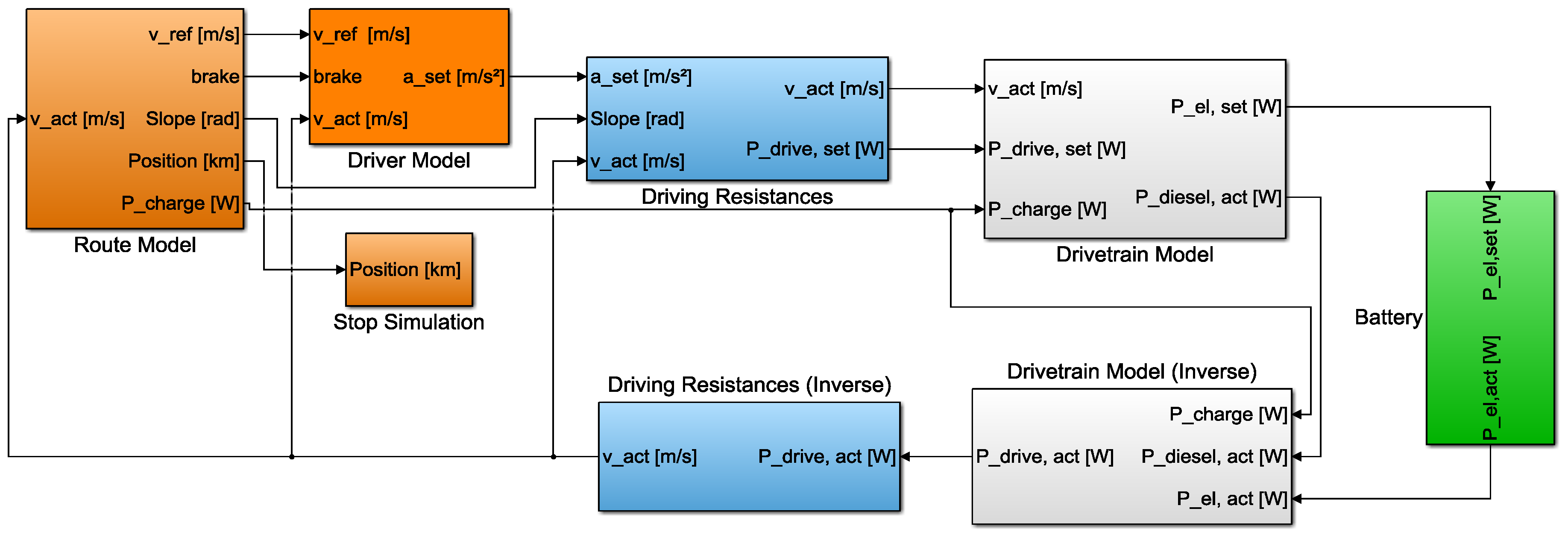
In order to estimate the energy consumption and to dimension the battery capacity a detailed simulation model of a battery electric truck was created. The model implementation in Matlab/Simulink R2015b (Natick, MA, USA) shown in
Figure 3 consists of a route model, driver model, driving resistances model, drivetrain model and battery model. Furthermore a graphical user interface was developed to parameterize the model and to analyze the simulation results.
First the route model imports a route profile that consists of GPS coordinates and elevation data as well as additional information that can be maximum driving speed, position of resting facilities, duration of rest periods and charging stations. Depending on the actual vehicle position the route defined signals are provided from route model to the following blocks. These signals are reference speed, slope, position, maximum charging station power and brake signal if a resting facility is reached or the reference speed is exceeded.
The driver model provides the set acceleration to meet the reference speed by accelerating or decelerating the vehicle. Provided the set acceleration, the slope and the actual velocity, the vehicle model calculates the set power
Pdrive, set to overcome the driving resistance that is the sum of air resistance, rolling resistance, slope resistance and acceleration resistance. The power
Pdrive, set is calculated according to the equations:
where
vact is the actual velocity of the vehicle. The air drag resistance force
Fair is calculated using the air drag coefficient
cw, the reference front area
A of the vehicle and the mass density
ρair of the air according to the equation:
The rolling resistance force
Froll is calculated according to the formula:
where
g is the gravitational acceleration,
mgross is the gross vehicle weight including the load,
croll is the rolling resistance coefficient and
α is the gradient angle. The slope resistance force
Fslope is calculated according to:
The acceleration force
Facceleration is calculated using the acceleration
aset and the sum of translational and rotatory contributions:
For the rotatory contribution to the acceleration force the mass of wheels mwheels and their dynamic radius rwheel as well as the rotating parts of motor and shaft JASM and the gear ratio igear are considered.
The drivetrain model contains two different drivetrain types: an electric drivetrain to simulate a battery electric truck and a diesel drivetrain to simulate a conventional diesel truck. The electric drivetrain for the battery truck consists of battery, converter, electric machine and gearbox. The resulting power transfer equation for the electric drivetrain is:
where
ηgearbox is the efficiency of the gearbox,
ηmot&conv is the efficiency of motor and converter and
Pel, set is the set power for the battery to deliver.
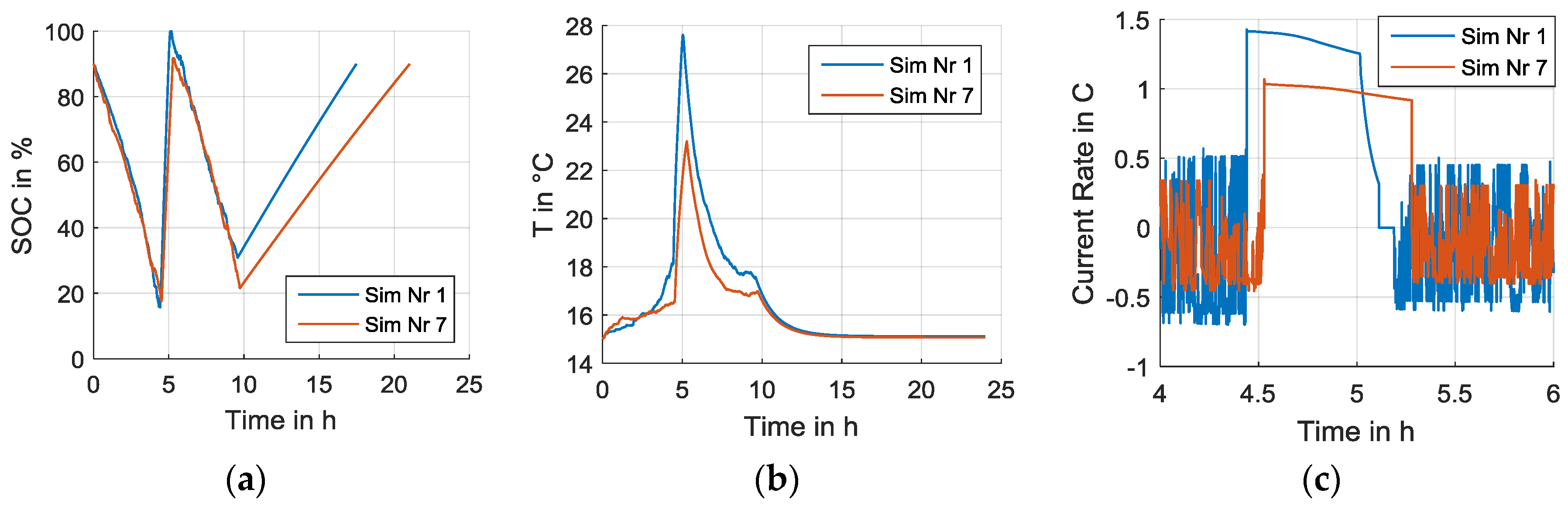
The battery model calculates the power
Pel, act that the battery can deliver depending i.e., on the parameters of the modeled cell, state of charge (SOC), temperature and actual state of health. The electric input and output of the traction battery is scaled to the model of a single cell (see
Section 2.3). This provides a detailed simulation of the battery calculating the voltage, current, SOC and temperature profiles for the simulated route that are used by the cell aging model after the driving simulation.
The conventional diesel drivetrain consists of the models for diesel motor and gearbox. The corresponding power transfer equation for the diesel drivetrain is:
where
Pdiesel, set is the set power for diesel motor to deliver.
After the actually deliverable battery power
Pel, act or diesel motor power
Pdiesel, act is calculated, the available power
Pdrive, act to overcome the driving resistances and the actual speed
vact are calculated (
Figure 3) using the Equations (1)–(7) and replacing the set values by actual values.
2.3. Parameterization of the Truck Simulation Model
The truck simulation model was parameterized for a heavy-duty semi-trailer truck with a gross vehicle weight of up to 40 t. As the rolling and air frictions essentially influence the energy consumption of the long-haul vehicle [
22], two truck configurations with different values for air and rolling drag coefficients are considered.
Table 1 shows the main parameters of the truck configurations “low losses” and “average losses” that were used to simulate the battery truck as well as the diesel truck. The used values for air drag and rolling drag coefficients correspond to the low and average values in the range given in [
23,
24] for European semi-trailer truck.
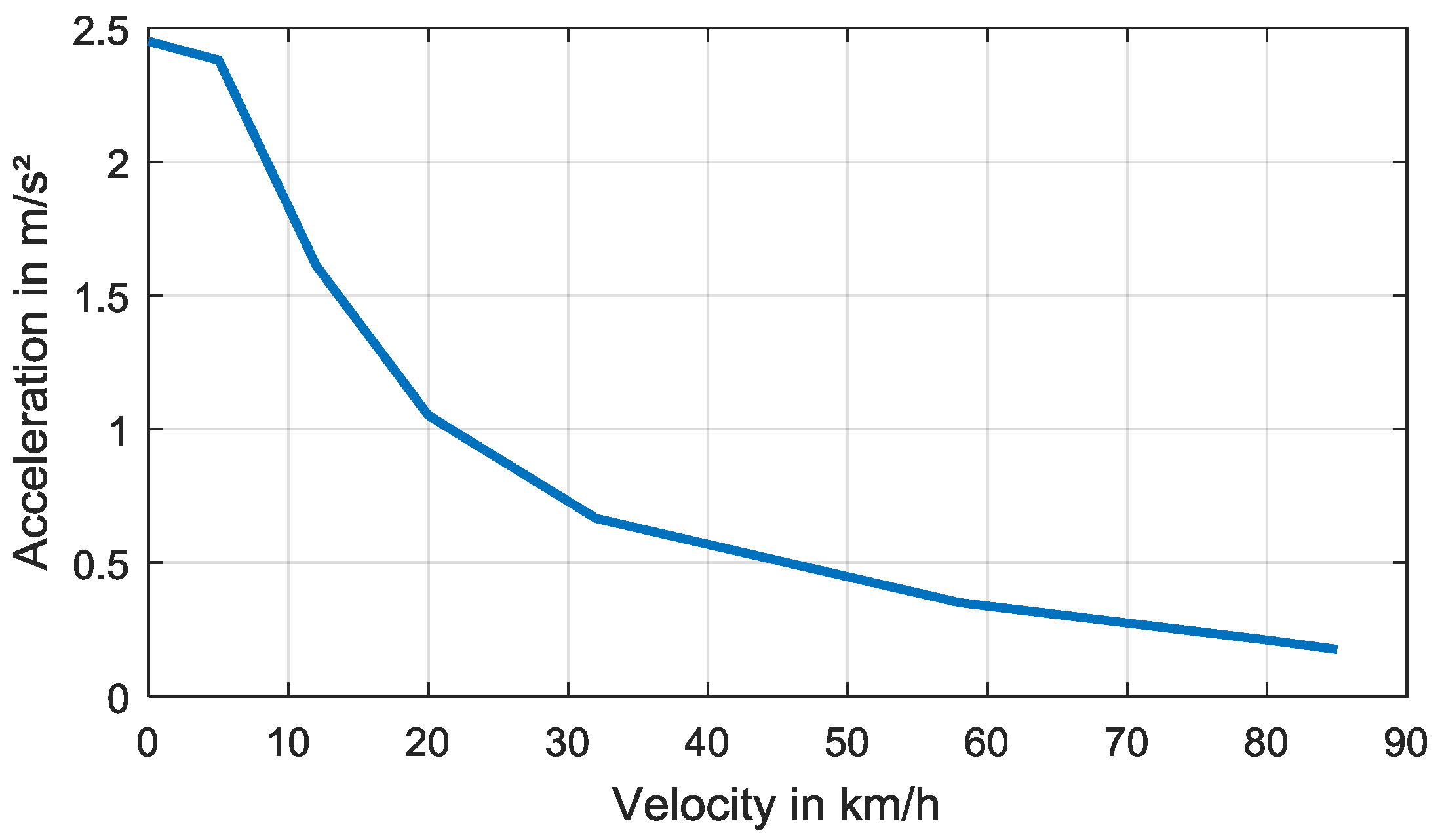
The driver model contains the acceleration and deceleration strategy for a heavy-duty truck. The set acceleration varies depending on the actual velocity as shown in
Figure 4. These values correspond to the acceleration of a 40 t diesel truck [
22] and multiplied with a factor 0.7 as it is assumed that the vehicle doesn’t accelerate at full power at standard driving situation. The deceleration is assumed to be constant at 0.9 m/s
2. The driver tries to meet the reference speed of the route by accelerating or decelerating the vehicle.
The electric machine and the according converter are implemented by the efficiency map depending on the shaft speed and torque of a three-phase permanent magnet electric motor [
25]. As the nominal power of this motor is 188 kW, two motors were implemented in the simulation model to provide the suitable power of 376 kW for a heavy-duty truck. To get the required torque, a gearbox with transmission ratios depending on the vehicle speed was implemented. The efficiency of the gearbox is assumed to be constant 0.94 which is an average value according to values given in [
26].
The used holistic cell model consists of the impedance based electric model, thermal model and aging model. It is parameterized for two cell types with data according to
Table 2 [
27,
28]. The cells use the same chemistry but differ in their housing forms, nominal capacities and maximum current rates as well as maximum number of cycles and battery costs. The current rate is defined as the current divided by the nominal cell capacity and provides a measure to compare currents of cells with different capacities. The maximum number of full cycles in
Table 2 is determined by the mathematical cell aging model described below at the ambient temperature of 15 °C and the current rate of 1 C until the end of life of the cell is reached which is usually defined by 20% capacity loss or by reaching the doubled internal resistance. The cycle number is determined and shown here to demonstrate the different lifetime capability of these cells and to assume the costs of batteries comprising the particular cell types. According to the actual battery prices [
8] and considering the numbers of full cycles, the costs of the batteries are assumed and given in
Table 2.
The electric cell model is described in detail in the study [
28] and represents the impedance based electric cell model consisting of an equivalent electric network with a series resistance, two ZARC elements and an open circuit voltage source. It is connected with the cell thermal model which calculates the cell temperature based on ohmic losses and heat transfer resistance for different mounting conditions [
28]. The cell aging model calculates the calendar and the cycle aging depending on the resulting cell voltage, current, temperature and state of charge and using the aging functions derived from the accelerated cell aging tests. The calendar and cycle aging are finally added to get the total cell aging [
28]. The holistic cell aging model was verified with profiles for city and highway driving matching the measurements well for capacity loss that is limiting the cell lifetime [
28].
For the conventional diesel drivetrain a diesel engine and a gearbox were implemented. The characteristic consumption curves of the diesel engine were scaled to fit the consumption values of a diesel motor with Euro VI emission standard for heavy-duty trucks [
29]. The implemented gearbox for the diesel engine includes 12 gear ratios and its efficiency was assumed to be equal to that of battery electric truck.
2.4. Dimensioning of the Traction Battery Capacity
To get an average value for the energy demand the battery electric truck was simulated on the main German highways A1 to A9. The GPS data for routes on these highways were gained from web mapping services [
30,
31] and completed with altitude profile from Shuttle Radar Topography Mission [
32].
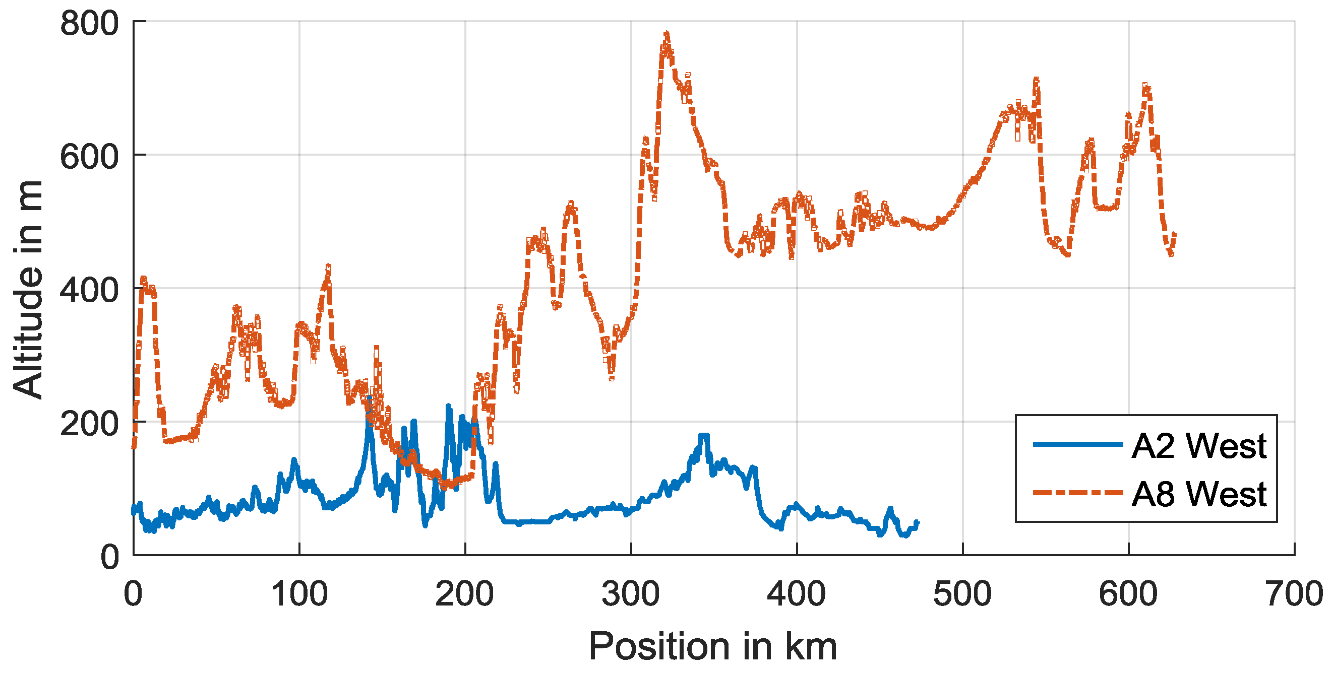
Figure 5 exemplarily shows the elevation profiles of two highways located in different German regions. The highway A2 is located in a rather flat region in the north of Germany and the highway A8 is located in a hilly region in the south of Germany which is reflected by a more alternating elevation profile. As the highways A1, A4 and A8 are not continuous, connecting country roads were used. The maximum allowed highway speed was set to 85 km/h and the traffic is not considered, so the differences in consumption values mainly result from different highway topologies and truck configurations according to
Table 1. The gross vehicle weight is set to 40 t not depending on the payload.
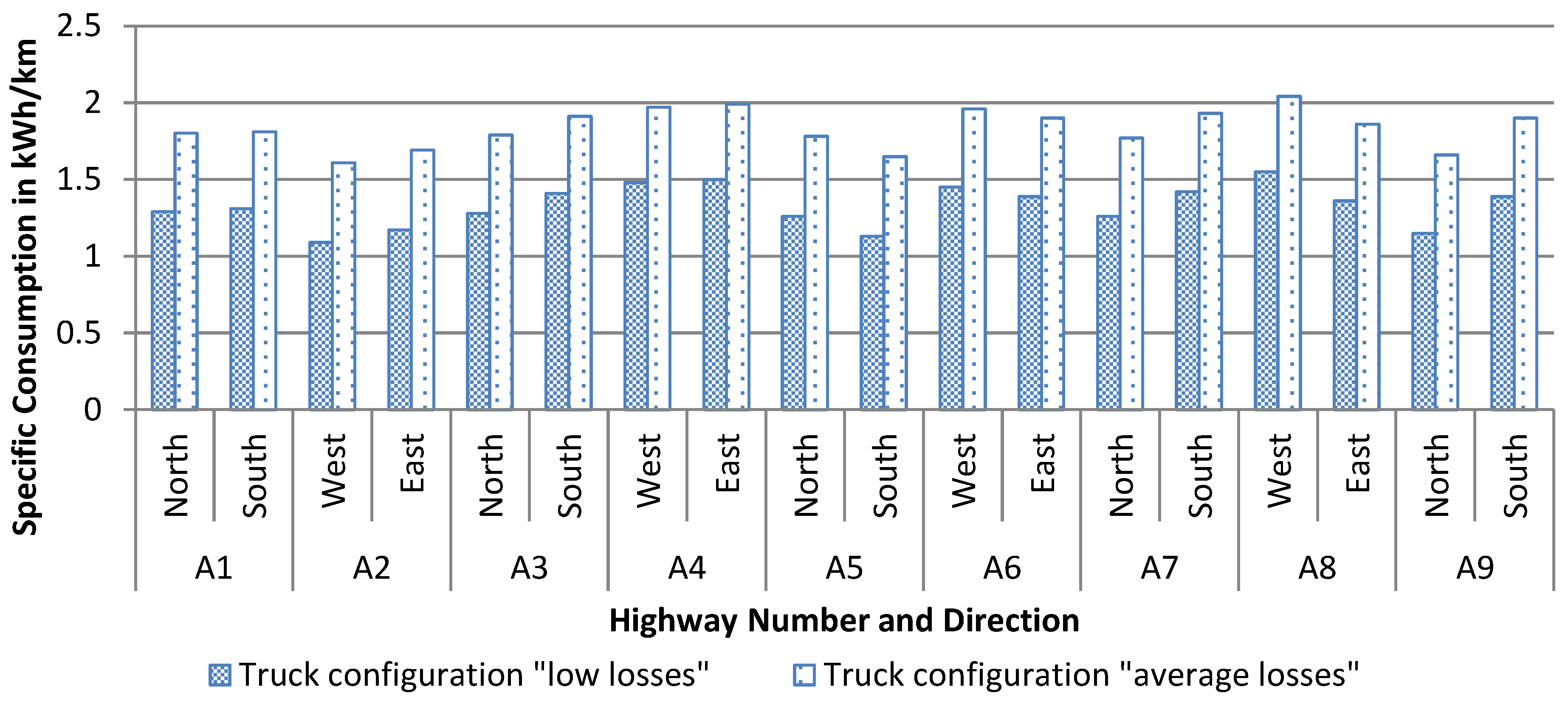
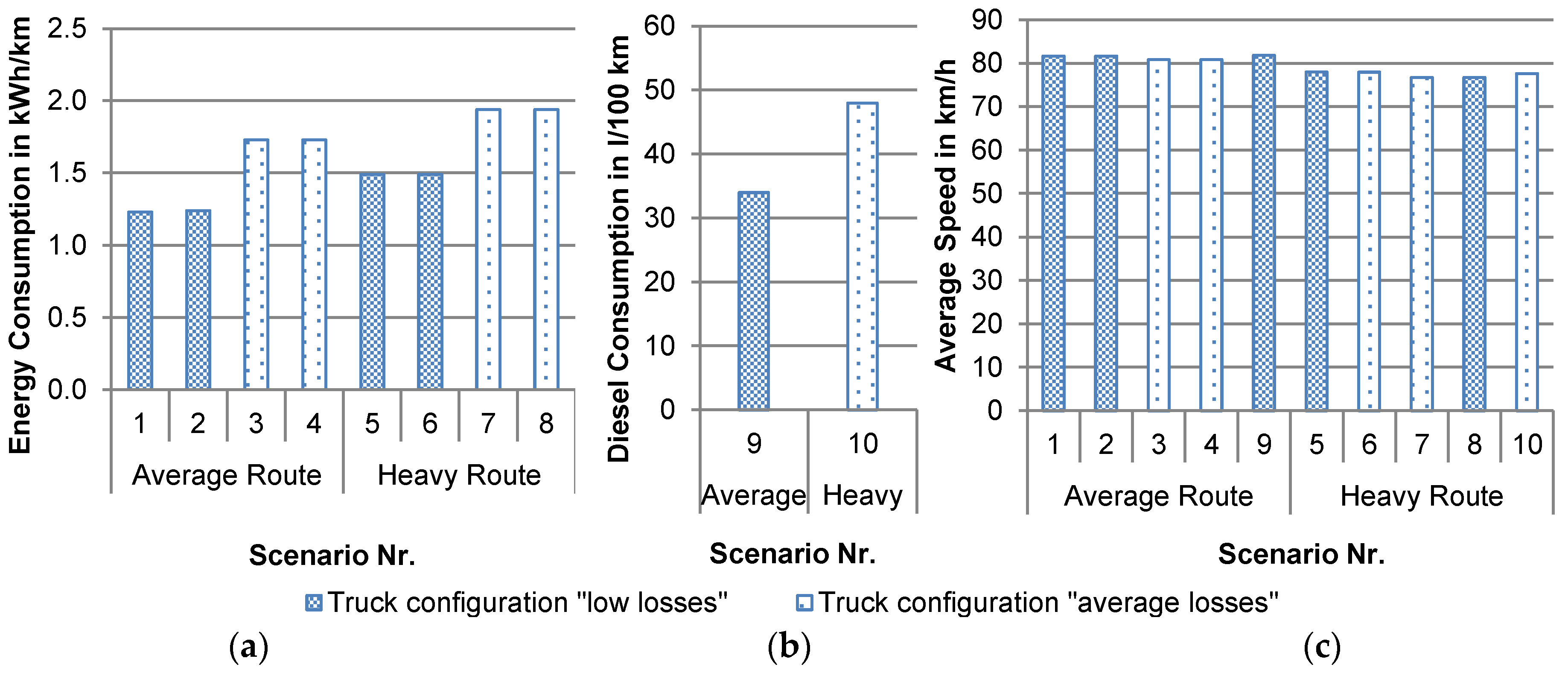
Figure 6 shows the simulated specific energy consumption for the truck configurations “low losses” and “average losses” according to
Table 1. The specific consumption varies from 1.09 kWh/km on highway A2 in direction west for the truck configuration “low losses” to 2.04 kWh/km on highway A8 in direction west for the truck configuration “average losses”. The consumption is in average about 28% smaller for the truck configuration “low losses” that shows the importance of low air and rolling drag coefficients. A low air drag coefficient can be reached by using i.e., side claddings, wind tunnels and roof spoiler while a low rolling coefficient can be reduced by choosing energy saving tires and maintaining the air pressure inside the tires [
23]. The average specific consumption calculated from all simulated trips results in 1.33 kWh/km for the truck configuration “low losses” and in 1.83 kWh/km for the truck configuration “average losses”.
According to the legislative conditions (
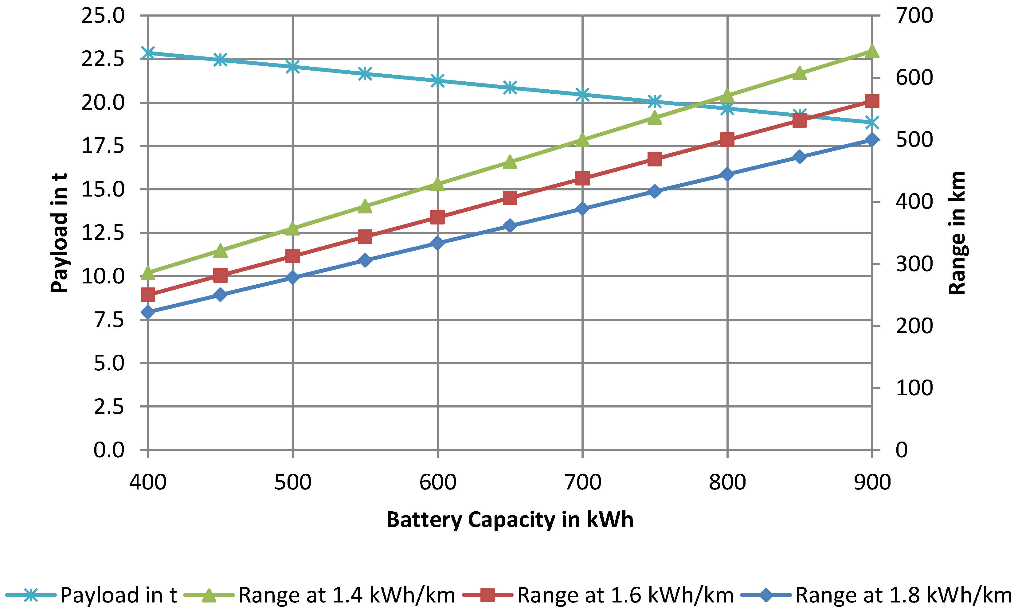
Section 2.1) the maximum driving period of a truck is 4.5 h, so the battery should be able to cover the corresponding route length and afterwards the battery can be charged during the driver’s rest period, provided there is a charging station at the rest facility. Assuming an average speed of 80 km/h a truck can cover 360 km within one 4.5 h driving period. Taking the calculated specific average consumption on highways for the truck configurations “low losses” and “average losses”, the required energy amount for one driving period is 478.8 kWh and 658.8 kWh, respectively.
In general the end of life of a battery is defined by 20% capacity loss or by reaching a doubled internal resistance. To account for the battery aging 20% of required energy amount for one driving period are added. This reserve is also suitable for the common truck operation and for varying truck parameters depending, i.e., on tire wear, weather conditions and traffic. Finally, the average required traction battery capacity to cover one 4.5 h driving period on the highway results in ca. 600 kWh for the truck configuration “low losses” and in ca. 825 kWh for the truck configuration “average losses”.
For the high consumption route with 2.0 kWh/km the required energy amount for one driving period is about 720 kWh, respectively, and considering the 20% reserve the resulting traction battery capacity is 900 kWh.
The determined battery capacities are significantly higher than the values of 270 kWh and 400 kWh assumed in comparable studies [
12,
13] due to the specified driving period and routes. The determined capacity values are used for the simulation of the transport scenarios specified in the next section and the integration of the traction battery into the truck is analyzed in
Section 3.2.
2.5. Definition of Transportation Scenarios
To calculate the life cycle costs of a battery electric truck and compare them to a diesel truck, two different transportation scenarios are considered. In the first transportation scenario a route with average consumption is considered while the second scenario considers a route with high consumption according to the results in the previous chapter.
Following legislative conditions (
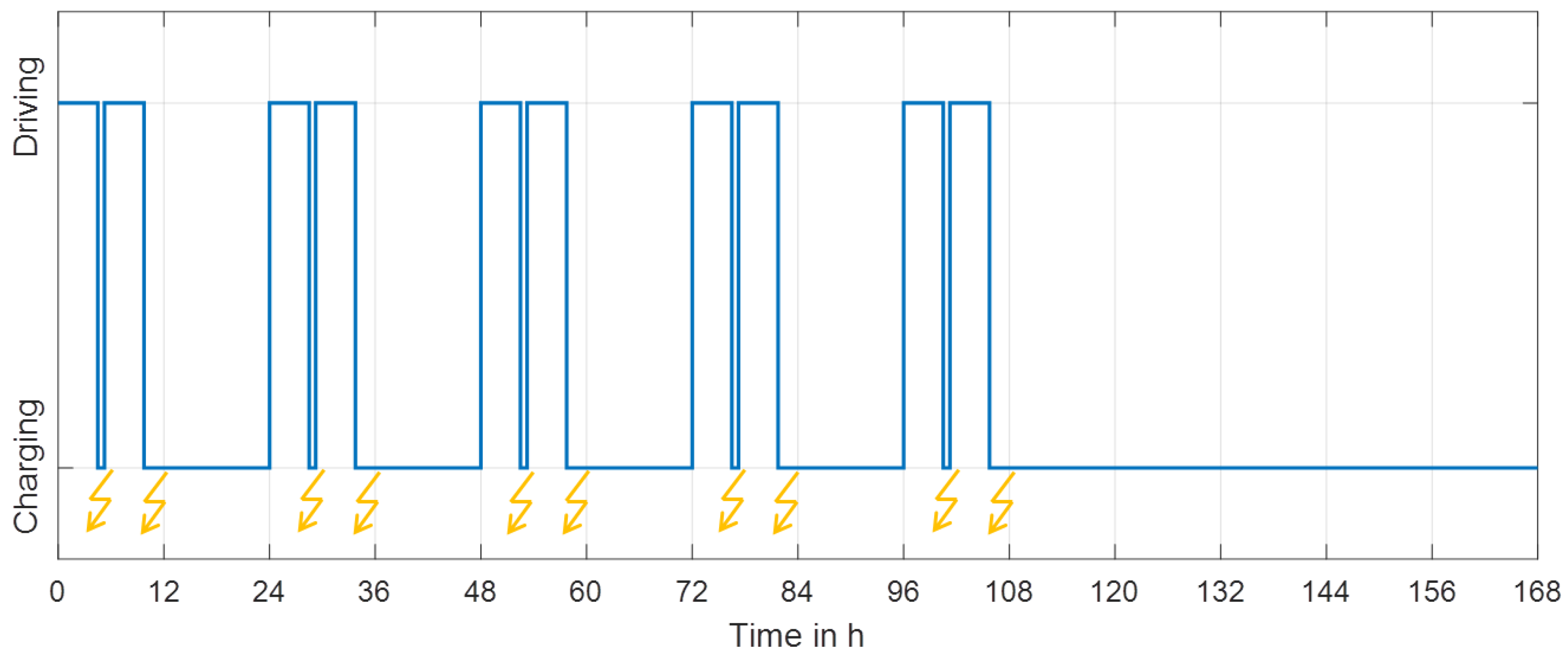
Section 2.1) a daily operation sequence of 4.5 h driving, 45 min rest period followed by the next 4.5 h driving period is assumed. The remaining daily time of 14 h 15 min is used for the rest period.
The 45 min rest period is used to fast charge the battery for the next driving period. The night rest period is used to charge the battery with low power, because of longer available time period. The slow charging at night would reduce the stress for the battery due to minor currents and minor temperature rise. The required charging power is calculated using the energy consumption on the route and the available charging time. The used charging method is charging with constant current and followed by charging with constant voltage (CC-CV). This method is used for the slow as well as for the fast charging to optimally use the driver’s rest period. The resulting daily driving sequence is shown in
Figure 7. Furthermore it is assumed that the truck drives the same daily sequence 5 days per week and 52 weeks per year. The resulting weekly driving sequence is also shown in
Figure 7.
For the daily driving sequence in the first transportation scenario a route with an average consumption is chosen. While for the second transportation scenario a route with high consumption was chosen.
Table 3 lists the main characteristics of these routes as well as the assumed truck payload. The shown altitude profiles of the routes in
Figure 8 as well as the underlying GPS data were gained from web mapping services [
30,
31] with altitude data provided from [
32].
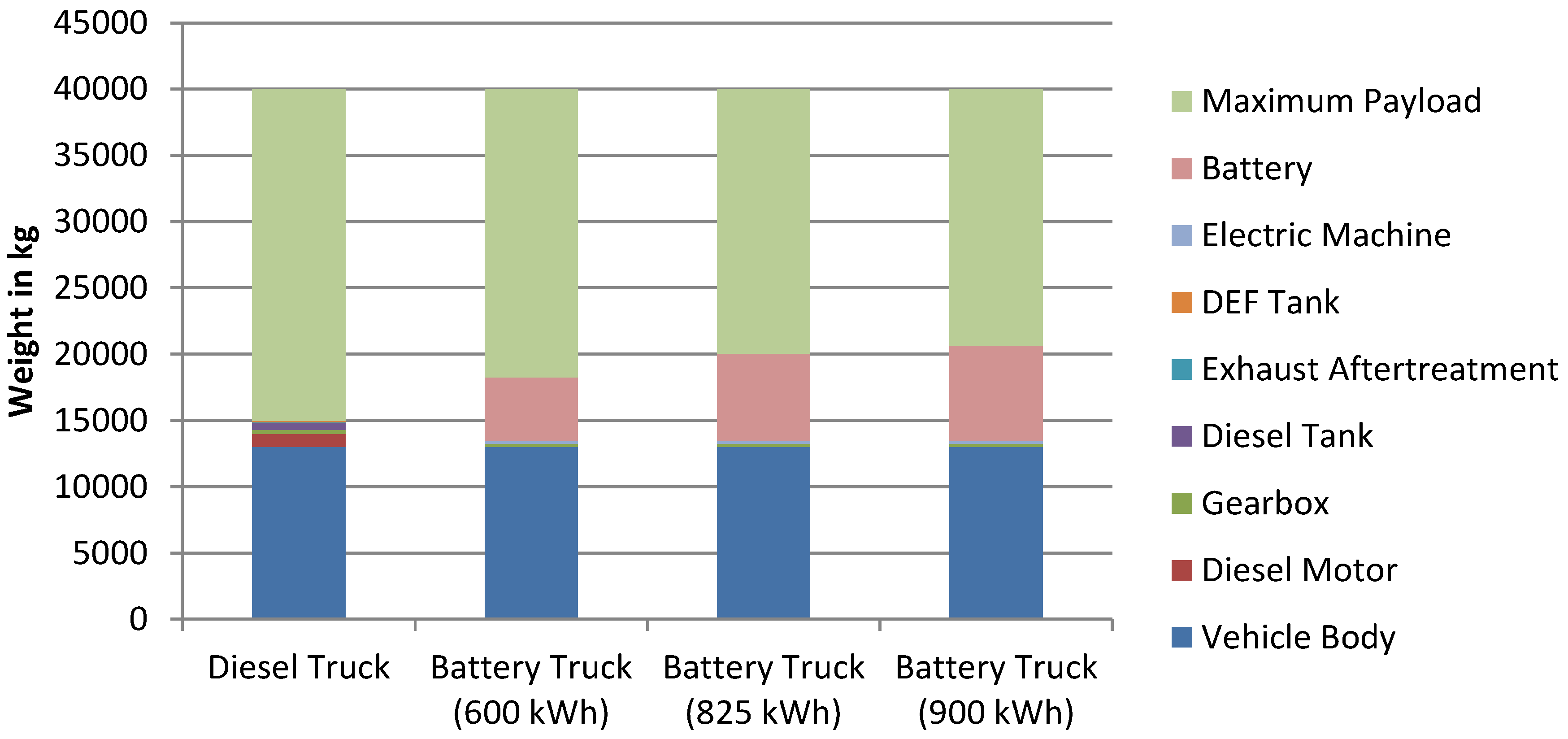
The described transportation scenarios are examined for the truck configurations shown in
Table 1 with 17.5 t payload for the electric as well as for the diesel truck. The same payload for different truck types is assumed to account for different maximum payloads as the traction battery with high capacity may restrict the available payload. This corresponds to the average payload usage of 70% for long-haul trucks (
Section 2.1).
2.6. Determination of Life Cycle Costs for Battery Electric Truck and Diesel Truck
To compare the battery electric truck and the diesel truck the life cycle costs (LCC) of both technologies are determined for the described transportation scenarios.
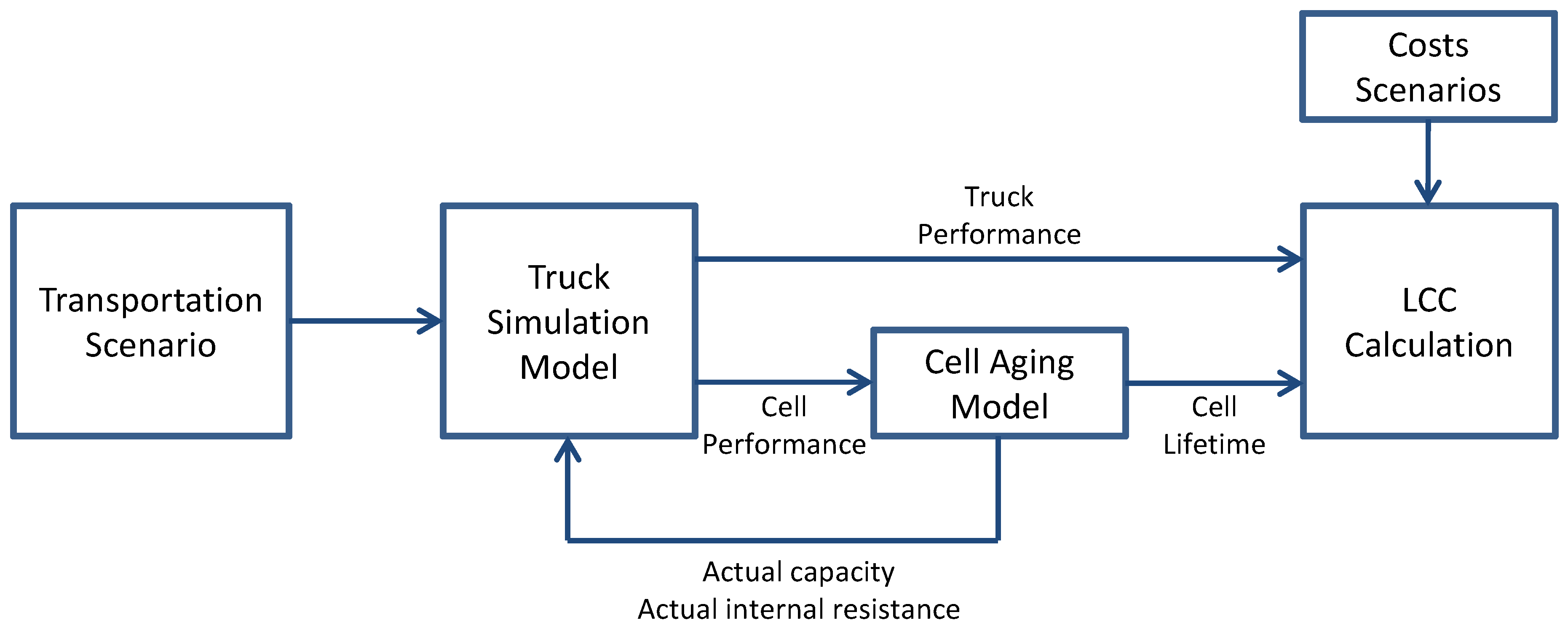
Figure 9 shows the data flow required for truck simulation and LCC calculation. The transportation scenarios containing the daily driving sequence and truck parameters are passed to the truck simulation model described in
Section 2.2. The truck simulation model provides: (i) the truck performance data containing the resulting velocity, components power and energy or diesel consumption, and (ii) the cell performance data containing the voltage, current, temperature and SOC of a battery cell used in the simulation. After running one simulation in the specified transportation scenario, the cell performance data is passed to the cell aging model [
28] and used to calculate the actual capacity and internal resistance of the cell. Both are calculated assuming an unaltered cell performance data for one year and then passed back to the truck simulation model to calculate the cell and truck performance for the next year. Finally after the cell reaches the end of life (80% of the initial capacity or a doubled internal resistance), LCC calculation is executed. It gets the truck and cell performance data as well as costs scenarios which are sets of cost parameters for the several components, energy, fuel, services and price developments.
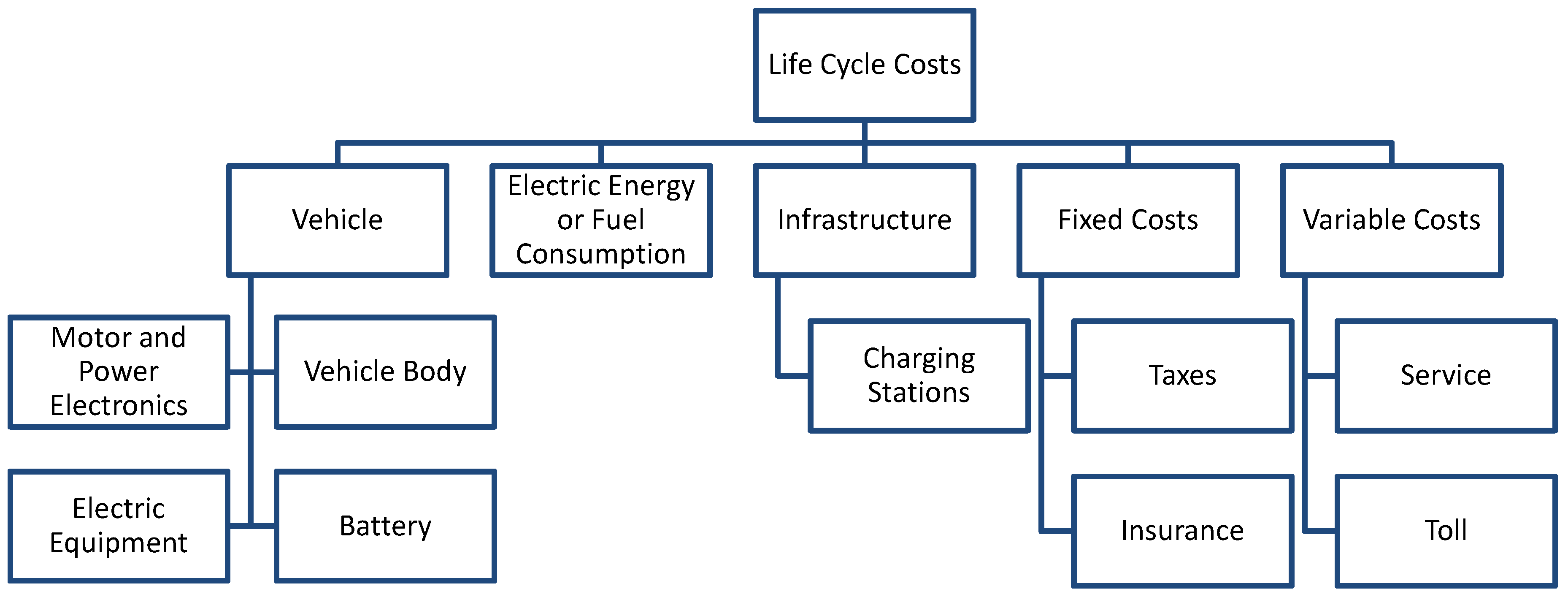
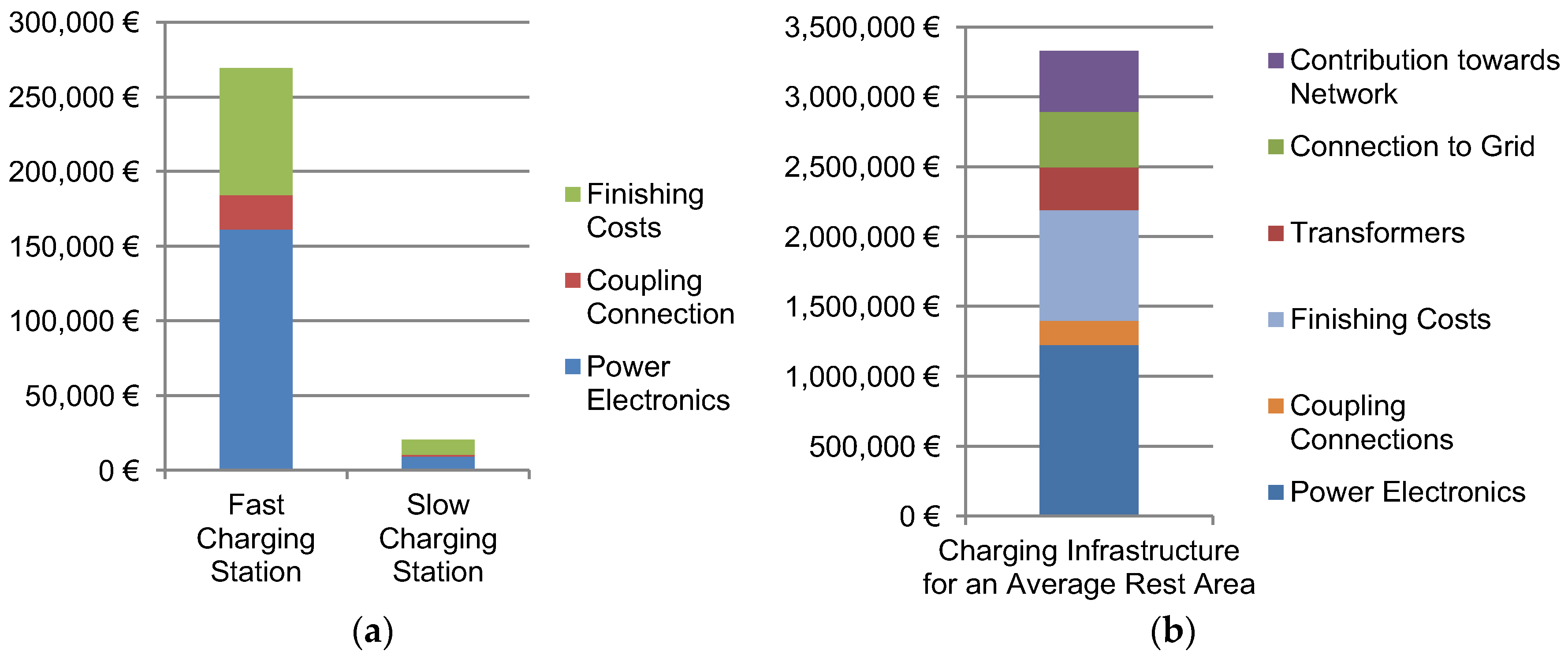
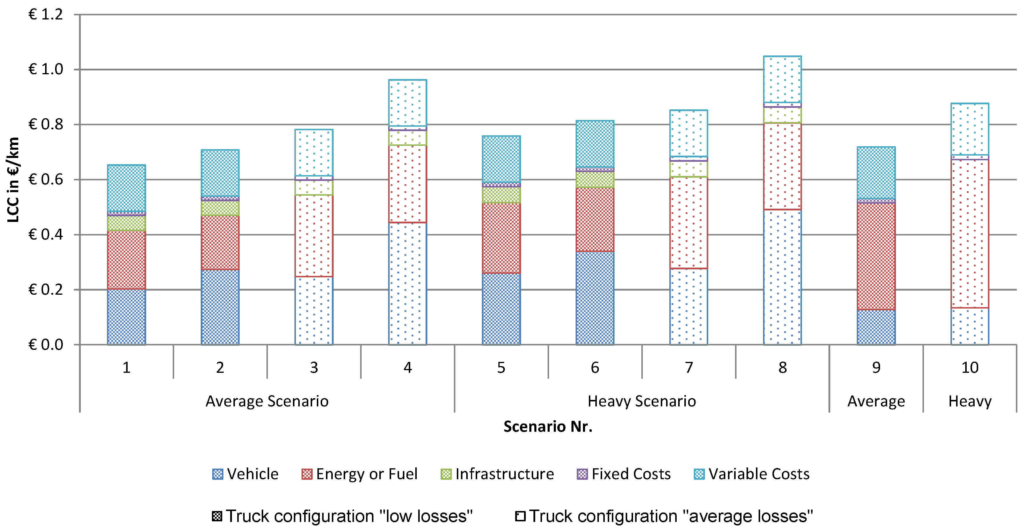
Figure 10 gives an overview of cost components considered in this calculation. Initially the costs for the vehicle which consist of vehicle body, battery, motor and electric equipment like power electronics and charging coupling are paid. The electric energy or fuel consumption is gained from the truck simulation model for a weekly driving sequence and scaled for the truck lifetime. For battery electric trucks the infrastructure is considered in terms of charging stations on the resting areas. For diesel trucks no infrastructure costs are calculated but considered as included into the diesel price. The fixed costs include annual taxes and insurance fees. The variable costs include fees that are depending on mileage and consist of service fees and toll.
Appendix A shows the main parameters for calculation of life cycle costs.
The LCC calculation is based on the net present value
NPV that is calculated for all components.
NPV provides the present value of future component costs
Ct depending on the interest rate
i and the residual value of the component
RVT. The
NPV is calculated using the formula:
where
t is the current year and T is the scenario duration. To account for different component lifetimes the residual value
RVT for truck components and charging infrastructure are calculated. The linear residual value progression is assumed according to the formula:
where
C0 is the component cost at the beginning of scenario,
Lrem, t is the remaining lifetime of the component,
L0 is the total component lifetime and
j is the inflation rate. The assumed inflation rate for the calculation is 1.39%/a and the assumed interest rate is 2.2%/a.
Finally
Table 4 summarizes the scenario combinations considered for LCC calculation. The LCC are calculated for the maximum mileage of 1,000,000 km that usually is the lifetime mileage of a conventional diesel truck. The last LCC calculations 9 and 10 are carried out for the diesel truck to compare the different drivetrain technologies.


