Abstract
Combined cycle power plants (CCPPs) are becoming more important as the global demand for electrical power increases. The power and efficiency of CCPPs are directly affected by the performance and thermal efficiency of the gas turbines. This study is the first unsteady numerical study that comprehensively considers axial gap (AG) in the first-stage stator and first-stage rotor (R1) and hot streaks in the combustor outlet throughout an entire two-stage turbine, as these factors affect the aerodynamic performance of the turbine. To resolve the three-dimensional unsteady-state compressible flow, an unsteady Reynolds-averaged Navier–Stokes (RANS) equation was used to calculate a turbulence model. The AG distance d was set as 80% (case 1) and 120% (case 3) for the design value case 2 (13 mm or d/Cs1 = 0.307) in a GE-E3 gas turbine model. Changes in the AG affect the overall flow field characteristics and efficiency. If AG decreases, the time-averaged maximum temperature and pressure of R1 exhibit differences of approximately 3 K and 400 Pa, respectively. In addition, the low-temperature zone around the hub and tip regions of R1 and second-stage rotor (R2) on the suction side becomes smaller owing to a secondary flow and the area-averaged surface temperature increases. The area-averaged heat flux of the blade surface increases by a maximum of 10.6% at the second-stage stator and 2.8% at R2 as the AG decreases. The total-to-total efficiencies of the overall turbine increase by 0.306% and 0.295% when the AG decreases.
1. Introduction
The global electrical power demand is expected to increase by 46% from 2015 to 2040, and this will lead to a large increase in electricity generation. Natural gas will be used for electricity generation instead of coal to minimize environmental problems caused by CO2 emissions. Electricity generation using natural gas is expected to increase from 5.22 trillion kWh in 2015 to 9.6 trillion kWh in 2040, an increase of 83.9%. Therefore, the importance of combined cycle power plants (CCPPs) that use natural gas is expected to considerably increase in the future. CCPPs consist of gas turbines that use natural gas and steam turbines that use steam, which is emitted from heat recovery steam generators. Increase in gas turbine power cause a similar increase of power in steam turbine and improves the overall efficiency of CCPP. The gas turbines’ aerodynamic performance and thermal efficiency have a direct effect on the cost of generated power of CCPPs.
One method of increasing gas turbine efficiency is to increase the turbine inlet temperature (TIT). However, a TIT distribution that is higher than the melting point of the material of the turbine blades results in a high thermal load on the turbine blades. Without a suitable cooling system, this leads to high-temperature corrosion and becomes a major factor in reducing the life of a turbine. To increase the TIT, it is necessary to more closely analyze the heat transfer characteristics of the surface of the turbine blade through an analysis of the transformed temperature distribution of the turbine inlet. The TIT distribution is directly affected by the fluid flow characteristics and temperature distribution of the combustor outlets. The temperature distribution of the turbine inlet is called a hot streak (HS), and it creates a complex heat transfer environment in the fluid flow passage and blade surface of the turbine [1]. HS has a different effect on the turbine blade surface compared with uniform temperature distribution; therefore, it is important to consider HS to analyze the overall performance and efficiency. As such, various numerical analyses and experimental studies have already been performed to describe the effect of HS on the heat transfer phenomena of a turbine blade. Butler et al. observed that high-temperature gas is concentrated on the pressure side of the rotor owing to an increased incidence angle and discovered points where the heat transfer effect is weakened [2]. Povey and Qureshi performed an experimental study on the temperature distribution in a combustor outlet and developed enhanced OTDF (EOTDF), which has a temperature distribution ratio of 1.65 [3]. EOTDF was used to create HS and they studied the influence of uniform temperature distributions at the turbine inlet as well as changes in the position of HS in the radial direction on the stator and rotor [1,4]. Bai-Tao An et al. studied the effect of uniform temperature distributions and HS inlet conditions on aerodynamic parameters such as total temperature, static pressure, and velocity [5]. Feng et al. found that the second-stage stator exhibits a high efficiency and low thermal load when its clocking position and HS were aligned [6]. Smith found that the time-averaged heat load when the HS is aligned with the stator had a large effect on the stator and a small effect on the rotor compared with the case when the HS is aligned with the stator passage [7]. However, these studies did not consider the effect of axial gap (AG) on the thermal and flow characteristics of the blade surface.
To increase gas turbine efficiency, it is important to analyze not only HS but also factors that affect aerodynamic performance. One factor that affects aerodynamic performance is the AG, i.e., a length of the straight line from the stator to the rotor. AG is a factor that directly affects the design and operation of turbomachines. It not only determines the overall size, length, and weight of a turbomachine but it also affects the unsteady flow in the rotor, noise, and aerodynamic performance of the turbine blade [8,9]. Furthermore, if the AG is too short, problems such as reduced fatigue life due to high inlet temperature occur. Therefore, experimental and numerical studies have been performed on the AG as an element that affects the overall turbine performance and efficiency. The AG affects the heat transfer coefficient (HTC) of the blade midspan in large-scale axial-flow turbines as well as the flow at the hub [10,11]. Funazaki performed an experimental and numerical analysis on changes in the flow angle in the stator outlet according to the AG in the first stage of the turbine [12]. Syed performed a numerical study on the composite effect of tip clearance and the AG of a stator blade in a multistage compressor [9]. It was found that changes in the first-stage stator and rotor AG affected turbine performance, but changes in the distance between the first-stage rotor and second-stage stator did not have a considerable effect on performance improvement. Previous studies found that as the AG becomes shorter, it affects the rotor torque and improves aerodynamic performance. However, they did not consider the thermal and flow characteristics in which the turbine blade surface is affected by the nonuniform temperature distribution of the turbine inlet according to the AG.
Accurate predictions of thermal and flow characteristics in a high-pressure gas turbine at the turbine blade and passage in more than one stage can have a considerable effect on turbine design. However, numerical investigations on multistage gas turbines are still expensive, and not many studies have been conducted thus far [13]. Adel performed a numerical analysis on a two-stage gas turbine with steady and unsteady states. The first stage was not affected by the second stage, but the second stage was strongly affected by the first stage. It was found that the upstream flow caused distortion in the downstream flow along the circumferential direction, and the flow interacts with the secondary flow and tip leakage flow of the blade [14]. Therefore, it is necessary to accurately understand the effect of the first stage flow on the second-stage and predict the thermal and flow characteristics within the passage and the heat transfer distribution of the blade surface.
Previous numerical studies for the AG effects applied uniform inlet temperature distributions to examine the aerodynamic performance of a turbine. Nonuniform inlet temperatures have been applied to predict the heat transfer distribution of the blade surface and the thermal and flow characteristics, but the AG was not considered. Furthermore, numerical studies that considered AG or HS have been performed on turbines with 1.5 or fewer stages. The gas turbine efficiency is affected by various design elements such as the AG and temperature distribution and varies in each stage. Therefore, this study performed a numerical analysis to investigate the effect of the AG on the thermal and flow characteristics of the blade surface and passage when an HS is applied to a two-stage turbine.
2. Numerical Method
2.1. Numerical Model and Grid
The gas turbine configuration used in this study is a GE-E3 gas turbine model. The actual gas turbine consists of 46 stators and 76 rotors in the first stage and 48 stators and 70 rotors in the second stage [15]. If one stator and two rotors have the same pitch angle, calculation errors during the numerical analysis can be minimized. As such, the number of blades was adjusted using a domain scaling method to create two rotors that correspond to the pitch of one stator in each stage [16]. In a state where the number of first stage rotors and the solidity of each blade are fixed, each chord length of the first stage stator (S1), second-stage stator (S2), and the rotor (R2) were magnified by 46/38, 48/38, and 70/76, respectively. Therefore, the number of blades used in the analysis was 38 for S1, 76 for the first stage rotor (R1), 38 for S2, and 76 for R2. Figure 1a shows the adjusted blade configuration for each stage and the computational domain used in this study, and Table 1 lists the information on each blade. The tip clearance of the rotor was 1% of the rotor height in R1 and 0.6% of the rotor height in R2.
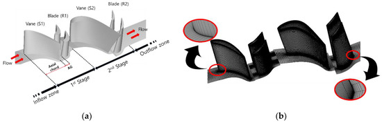
Figure 1.
Two-stage stator and rotor geometry details (based on GE-E3 (General Electric-energy efficient engine geometry [15]) turbine) (a) computational domain with domain scaling, and (b) computational grid of domain.

Table 1.
Information on GE-E3 turbine and domain.
In the numerical analysis, Ansys Turbogrid was used to create a hexahedral grid as shown in Figure 1b. To accurately predict the thermal and flow characteristics within the boundary layers, y+ was set to less than 1 at all walls and less than 0.5 at the blade surface. A grid independence test was performed to determine the appropriate number of grids to be used in the study. Table 2 lists the number of meshes (to achieve the equal domain pitch angle, the R1, R2 meshes in the list is doubled) used in the test and the area-averaged heat flux of the blade. In the grid independence test, grids were created for each blade by multiplying 1.34 times based on Mesh-1. In Mesh-1 and 2 and Mesh-2 and 3, the relative errors of the area-averaged heat fluxes were both under 0.01% for S1, and they were 0.75% and 0.41% for R1, respectively; thus, the Mesh-2 grid was used for S1 and R1. In Mesh-2 and 3 and Mesh-3 and 4, the relative errors of area-averaged heat flux where 1.83% and 0.41% for S2, respectively, and 1.79% and 0.8% for R2, respectively, so the Mesh-3 grid was used for S2 and R2.
Table 2.
Area-averaged heat flux at the surface of the four-row airfoil for applying the appropriate domain mesh (Mesh-2 is applied for 1st stage stator (S1) and rotor (R1), and Mesh-3 is applied for 2nd stage stator (S2) and rotor (R2)).
2.2. Numerical Details and Boundary Conditions
A continuity equation, momentum equation, and energy equation were used to analyze the compressible fluid flow of a three-dimensional unsteady state. These equations can be expressed as Equations (1)–(3), respectively.
Here, is the fluid’s density. is the fluid’s velocity. is the fluid’s pressure. is the fluid’s viscosity. In Equation (3), is the specific internal energy. is the effective thermal conductivity. is the specific heat capacity. is the effective dynamic viscosity. To accurately predict the flow separation phenomena, a turbulence model was used. To solve the governing equation, a commercial computational fluid dynamics software ANSYS CFX was used.
The boundary conditions used in this simulation are indicated following the GE-E3 turbine test performance report [15], air was used as the working fluid, and a total pressure of 344,740 Pa was used at the inlet and a static pressure of 50,000 Pa was used at the outlet. The rotor’s rotation speed was 3600 RPM. At the inlet, the Mach number was 0.11 (45.1 m/s). The Reynolds number was 210,000 based on S1’s axial chord length (Cs1 = 42.4 mm). The inlet turbulence intensity was set as 5%. A no-slip condition was used on the wall surfaces. To calculate the HTC, simulations for both isothermal and adiabatic wall conditions were conducted. Under the isothermal wall condition, the turbine blade temperature was 389.95 K.
To analyze the internal thermal and flow characteristics according to the inlet temperature field, a nonuniform HS inlet temperature condition with a maximum temperature of 838 K at the center was used, and a uniform inlet temperature condition with a temperature of 728 K was used, as shown in Figure 2. In addition, to examine the effects according to the AG when an HS was applied, three cases were analyzed in which the distance of AG, d, of S1 and R1 was set as the design value (case 2: 13 mm or d/Cs1 = 0.307), 80% of the design value (case 1: 10.4 mm or d/Cs1 = 0.245), and 120% of the design value (case 3: 15.6 mm or d/Cs1 = 0.368).
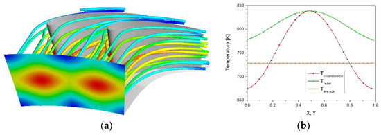
Figure 2.
Temperature profile at the turbine inlet: (a) hot streak (HS) temperature contour with streamlines, and (b) circumferential, radial, and average temperature distributions.
For numerical simulations, a 96-core workstation (4 Intel(R) Xeon(R) CPU E7-8890 v4 @ 2.20 GHz, RAM 512 GB) and a 44-core workstation (2 Intel(R) Xeon(R) CPU E5-2699 v4 @ 2.20 GHz, RAM 256 GB) were used, and the computation time required for a case was about 60 hours when using the 36-core.
2.3. Unsteady State
A steady state analysis was performed by setting the rotor–stator interface as a frozen rotor, and the results were used as the initial conditions for the unsteady state analysis. The transient rotor–stator model was used for the rotor–stator interface for the unsteady simulations. The pressure values of R1 at the midspan were compared among 16, 32, and 50 time step unsteady simulations to determine the step of each cycle in which one R1 completely passes through a pitch of S1. Figure 3 shows the pressure distribution plot at the 4.7° and 9.45° positions when the 1 pitch angle of S1 is 9.45°. The relative error rate was calculated by substituting the pressure value of each step at the R1 midspan in Equations (4) and (5) below.
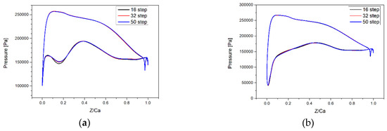
Figure 3.
Comparing pressure differences between 16, 32, and 50 time step simulations for each angle on the R1 midspan to find the appropriate step in the unsteady state flow analysis: (a) θ = 4.7°, and (b) θ = 9.45°.
The maximum relative error rates at the 16 and 32 time-step simulations were 3.22% at R1 position 4.7° and 6.81% at 9.45°. The mean relative error rates were 1.27% at 4.7° and 0.43% at 9.45°. The maximum relative error rates at 32 and 50 time-step simulations were 1.27% at 4.7° and 4.28% at 9.45°. The mean relative error rates were 0.25% at 4.7° and 0.25% at 9.45°. The maximum and mean relative errors at 32 and 50 time-step simulations were significantly reduced compared with those at 16 and 32 time-step simulations. Thus, 32 time steps for one pitch were used in each cycle to perform the unsteady state flow analysis.
The temperature and pressure at one point near each blade pressure side wall were monitored to confirm periodically constant convergence state. The initial 20 pitches were excluded as the initial transient from the total 30 pitches’ unsteady state simulation, and the remaining 10 pitches were used in the analysis of the results. Figure 4 shows the temperature and pressure measured for eight pitches, excluding the initial transient. The pressure and temperature for each pitch cycle (=32 time steps) in the unsteady state analysis appear to be periodic.
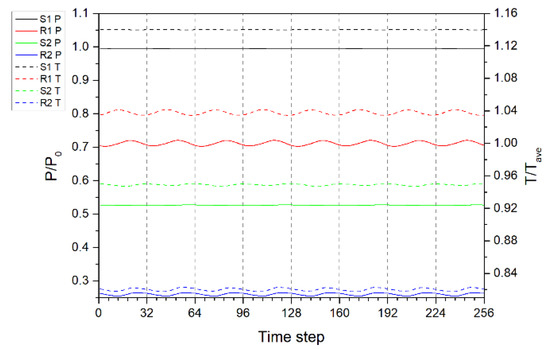
Figure 4.
Periodic variation in temperature and pressure at four monitoring points (32 steps = 1 pitch, P0 = 344,740 Pa, Tave = 728 K).
2.4. Validation of the Turbulence Model
Deciding the appropriate turbulence model is important for more precise numerical analysis. Direct numerical simulations (DNS) and large eddy simulations (LES) provide a flow database for detailed turbulence statistics, but they require a high computational cost [17,18,19,20,21]. To replace such high-cost models, a Reynolds-average Navier-Stokes (RANS) model ( etc. …) is used in turbomachinery simulation and especially, and transition models can predict more accurate transitional flows [22,23]. To determine the turbulence model for this study, a steady state analysis was performed. The validation for the model was performed using the relative pressure and HTC in comparison with Hylton’s experiment values [24]. The configuration and boundary conditions can be seen in the experiment section of Hylton et al. [24]. The 50% span experiment values of the C3X cascade No. 4311 experimental stator were used for comparison. As for the computation domain used in validation, the inflow zone, which is between the inlet and the stator leading edge (LE), was set to be same as the C3X vane axial chord (AC), and the outflow zone, which is between the trailing edge (TE) and the outlet, was set at twice the AC. A grid independence test was performed and 4,015,728 hexahedron meshes were applied. The boundary conditions used in the simulation were set such that the uniform inlet condition’s total pressure was 244,763 Pa, the Mach number was 0.17, the Reynolds number based on the C3X vane’s AC was , the temperature was 802 K, and the turbulence intensity was 6.5%. The outlet conditions were set such that the static pressure was 131,800 Pa, and the outlet Mach number was 0.91. To calculate the HTC, simulations with adiabatic and isothermal wall (temperature 537 K) conditions were conducted. The HTC in this study was calculated using Equation (6), as given below:
In Equation (6), is the heat flux in the isothermal wall simulation, is the wall temperature value in the adiabatic wall simulation, is the blade temperature value for the isothermal case, and is the HTC. In Figure 5, the relative pressure and the HTC value of 50% span of the stator found in the experiment paper [24] are compared to the values found from using the , , , and turbulence models used in this study. For the relative pressure distribution in Figure 5a, the pressure at the C3X vane midspan normalized by the inlet total pressure P0 were used. The comparison revealed a strong agreement between the simulations and experimental data. A relatively larger difference in the area of the suction side (SS) is attributed to the strong unsteadiness of the flow. Figure 5b shows the HTC distribution. In the , , and turbulence models, the SS transition region was different from the experiment values. The turbulence model shows a similar tendency with regard to the experiment values overall, including the SS transition regions. Therefore the turbulence model was used in this study with the onset Reynolds number of 150 [23].
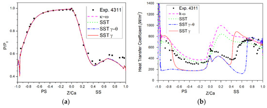
Figure 5.
Comparison of experimental data with different turbulence models at 50% span of C3X vane (experimental geometry [24]): (a) relative pressure distribution (P0 = 244,763 Pa), and (b) heat transfer coefficient (HTC) distribution.
3. Results and Discussions
3.1. Effect of Inlet Temperature Field
To examine the effect that the turbine inlet temperature conditions have on the blade, two steady state analyses were performed under uniform and nonuniform temperature conditions. In the uniform conditions, the turbine inlet temperature was maintained at 728 K. In the nonuniform conditions, the temperature distribution was nonuniformed with an average inlet temperature of 728 K, as shown in Figure 2. Figure 6 shows the surface temperature distribution of the S1 surface’s according to each inlet condition on adiabatic walls. In the uniform inlet temperature conditions shown in Figure 6a, the maximum temperature was approximately 729 K, and the temperature distribution showed a trend of decreasing at the PS in the streamwise direction. In Figure 6b, it can be seen that the high temperature gas was centered on the midspan because of the temperature distribution caused by the HS. It is also clear that the high temperature gas formed in the radially inward direction due to the secondary flow transport effect that occurs at the tip and hub near the trailing edge of the SS. This led to fluid-mixing at the stator endwall and the temperature became lower around the hub and tip of the S1 TE. When an HS was applied, the S1 maximum surface temperature was 839 K, which shows a difference of over 110 K compared to the uniform inlet conditions.
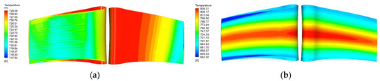
Figure 6.
S1 surface temperature contour caused by inlet conditions (Right is pressure side (PS)): (a) uniform inlet temperature of 728 K, and (b) HS with an average temperature of 728 K.
Figure 7a shows a comparison of the temperature distributions along the span direction at AC 50% in the PS of S1 and R1. When a uniform temperature distribution was applied, there were few temperature changes along the span direction in S1 and R1. When an HS was applied, higher temperatures are observed at the midspan than around the endwall in S1 and R1. Furthermore, the temperature between 20% and 70% of the span of R1 was higher than the temperature of S1 when a uniform temperature was applied. The maximum temperature differences according to the inlet conditions were 110 K and 75 K for S1 and R1, respectively. Both Figure 7b,c shows the temperature contours at the first midspan according to each inlet temperature condition. Overall higher temperatures were observed in Figure 7c as compared to Figure 7b. Compared to the uniform inlet temperature distribution, the HS inlet temperature gradient, which formed differently along the radial and circumferential directions, had a direct effect on the overall temperature distribution of the blade. Figure 6 and Figure 7 show that it is important to consider the HS inlet conditions in the numerical analysis to understand the thermal and flow characteristics.
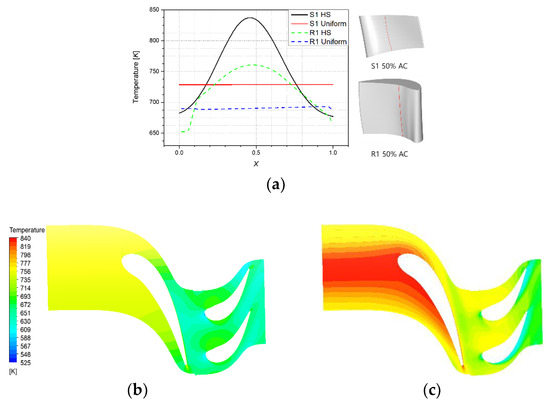
Figure 7.
Temperature distribution and contour on the first stage with different inlet condition: (a) temperature distribution on S1, R1 PS axial chord (AC) 50%, (b) uniform inlet temperature of 728 K at the midspan, and (c) HS with an average temperature of 728 K at the midspan.
3.2. Flow and Thermal Characteristics at R1, R2
Flow in a turbine passage affects the surrounding blade surfaces. Figure 8a–c shows the time-averaged streamline of the SS for the surface of R1. Figure 8d–f shows the time-averaged streamline of the SS for the surface of R2. Compared to the PS where the S1 downstream flow acts directly, the flow characteristics of the surface according to the AG were greater at SS. In the figure, the part indicated with the solid line is the recirculation zone. If Figure 8a,c is compared, it can be seen that the AG was reduced (from c to a), and recirculation zone became larger and farther from the LE. This is because in case 3 the mass flow at the tip was 6.32 g/s and in case 1 it was 6.42 g/s. Thus, the mass flow that passes through the tip clearance increased by 1.61%. Owing to the decreased AG, the total pressure at the front of the R1 LE was 219,828 Pa for case 3 and 222,395 for case 1, which is an increase of 1.16%. In the R2 surface’s time-averaged streamline, the flow effect at R2 was distributed such that the effect of the secondary flow and recirculation zone was not observed, unlike R1, which was strongly affected by the inlet. As the AG reduced, some streamlines formed downward from the tip (Figure 8d), as opposed to the most streamline formed around the LE in Figure 8f. The change in the AG of S1 and R1 is a factor that affects the rotor surface flow and the creation of secondary flow at the turbine passage after R1 owing to changes in the mass flow at the tip and R1 LE’s total pressure.
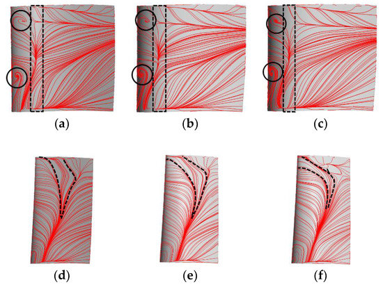
Figure 8.
Surface streamlines on R1, R2 suction side (SS): (a) R1 case 1, (b) R1 case 2, (c) R1 case 3, (d) R2 case 1, (e) R2 case 2, and (f) R2 case 3.
These phenomena are also caused by a difference in velocity distribution in the main flow of the S1 downstream as the HS passes S1 until it reaches R1. Figure 9 shows the time-averaged velocity distribution at the R1 inlet for each case. The part indicated by the dotted line is where the S1 downstream flow exhibits high-speed flow in the vicinity of the R1 LE. As the AG decreases, the area with higher velocity forms from the midspan to the hub and exerts its influence.
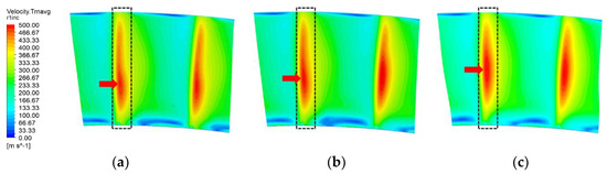
Figure 9.
Time-averaged velocity profile at R1 inlet in three cases: (a) case 1, (b) case 2, and (c) case 3.
Figure 10 shows the time-averaged temperature contours of the PS and SS of the surface of R1. At the PS, where the HS turbine inlet condition is primarily concentrated, a high temperature area was observed; however, the effect of the axial gap was not large. At the SS, the high temperature area became larger at the TE in Figure 10a compared to Figure 10c owing to the secondary flow and tip leakage flow around the tip and hub as shown in Figure 8. Figure 11 shows the temperature distribution along the span at AC of 50% and 80% of the SS. Observing the effect that the AG had on the SS surface temperature, it can be seen that the effect of the tip leakage vortex at the tip was larger than the effect of the secondary flow at the hub. Near the tip, case 3 (in which the AG was large) was lower than case 1 by a maximum of 27 K at AC of 50% and a maximum of 43 K at AC of 80%.
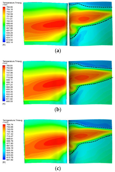
Figure 10.
Time-averaged temperature contours on R1, PS, and SS (Left is PS) (a) case 1, (b) case 2, and (c) case 3.
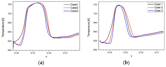
Figure 11.
R1 SS span direction temperature distribution: (a) AC 50%, and (b) AC 80%.
The time-averaged temperature and pressure distribution results for each R1 were compared to analyze the thermal and flow characteristics according to the AG in a two-stage gas turbine under HS inlet conditions. Figure 12 shows the area-averaged and maximum temperature and pressure of the surface of R1. The time-averaged values in the area-averaged temperature distribution shown in Figure 12a were 689.15 K for case 1 and 687.69 K for case 3, which shows a difference of approximately 1.5 K. The maximum temperature distributions of case 1 and case 3 differed by over 3 K. The area-averaged pressure distributions in Figure 12b were 181,601 Pa for case 1, which has a short AG, and 179,779 Pa for case 3. This yields a difference of approximately 2000 Pa. In the maximum pressure distributions, there was a difference of approximately 400 Pa between case 1 and case 3, and a relatively small difference compared to the area-averaged pressure distribution was observed. Overall, a trend can be seen in which the AG decreased and the area-averaged and maximum pressure and temperature increased.
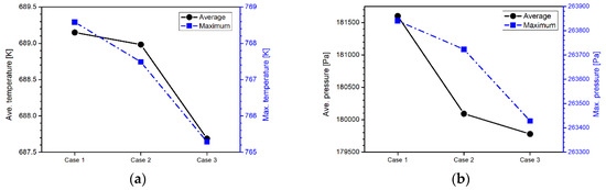
Figure 12.
Time-averaged temperature and pressure distributions on R1 surface in three cases: (a) the distribution of area-averaged and maximum temperature on R1 surface, and (b) the distribution of area-averaged and maximum pressure on R1 surface.
3.3. Effect of Heat Flux on the Vane and the Blade Surface
The heat flux characteristics of the turbine blade can be understood by accurately quantifying the heat flux regions of each blade according to the AG, and a cooling technology can be developed accordingly. Figure 13 shows the time-average heat flux contour of the R1 and R2 surfaces. In the R1 PS shown in Figure 13a, in which the AG becomes close, it can be seen that the low heat flux region from the tip to the 40% span was reduced compared to Figure 13c. Furthermore, the low heat flux region that extended to an AC of 80% was reduced to an AC of 50% in Figure 13a. On the SS, there was a high heat flux around the LE in Figure 13a. When it moved to the TE side, and a contour formed in the radially inward direction and heat flux became lower. However, in Figure 13c, which has a long AG, a lower heat flux was formed at the LE than in Figure 13a, and a low heat flux region was centered on the TE. At R2’s PS, the AG became closer, and the heat flux increased on the LE near the turbine hub. It was centered on the hub to mid span. The low heat flux region at 30% span formed at 40% span and the heat flux increased. On the SS, the AG became closer and heat flux increased at 20% span.
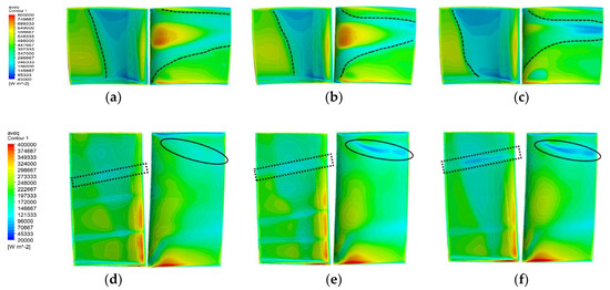
Figure 13.
Time-averaged R1, R2 surface heat flux contour (Left is PS): (a) R1 case 1, (b) R1 case 2, (c) R1 case 3, (d) R2 case 1, (e) R2 case 2, and (f) R2 case 3.
Figure 14 shows the time-averaged distribution of the area-averaged heat flux for each blade (including the tip). At S1, the heat flux based on the AG showed a difference of less than 0.1%, thereby confirming that the S1-R1 AG did not have a significant effect on S1. At S2 and R2, the heat flux increased by 10.6% and 2.8%, respectively, as the AG decreased from case 3 to case 1. At R1, the heat flux was slightly lower in case 1 than in case 2. This is because the area-averaged heat flux at case 2’s tip was higher than that of case 1. At the second-stage of S2 and R2, as the AG became closer, the heat flux became larger and the effect on the surface became larger.
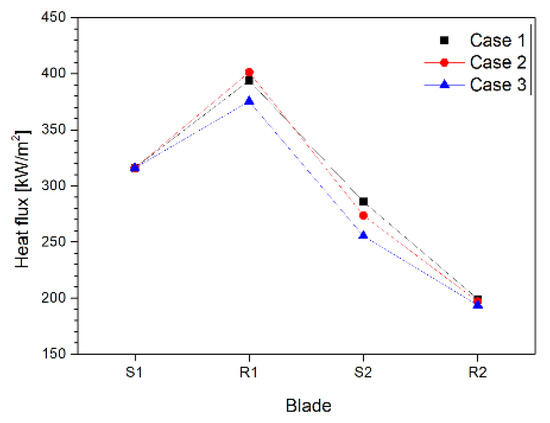
Figure 14.
Area-averaged heat flux on the surface of S1, R1, S2, and R2.
3.4. Total-to-Total Efficiency
To quantitatively evaluate the aerodynamic performance of the two-stage turbine with regard to the AG, the total-to-total efficiency was calculated. The efficiency was calculated using Equation (7):
Here, is the total-to-total efficiency, is the torque, is the angular velocity, is the mass flow rate, is the specific heat capacity of the turbine inlet, is the mean temperature of the turbine inlet, is the mass-averaged total pressure of the turbine outlet, is the total pressure of the turbine inlet, and the is the ratio of specific heat. Both and directly affect the efficiency whereas other parameter values remain constant throughout the whole cases. The X axis in Figure 15 indicates that the AG distance was divided by the axial chord length of S1, and the Y axis indicates the efficiency, torque, and pressure outlet () normalized by the value of case 2. The normalized values of efficiency, torque, and pressure outlet in cases 1 and 3 are 1.00295 and 0.99694, 1.00218 and 0.99735, and 1.00171 and 0.99911, respectively. The efficiency according to the decrease in the AG was increased. As the AG decreases, the turbine efficiencies increased by 0.306% and 0.295% for case 2 and case 1, respectively. In case 1, which had the shortest AG, the efficiency was 0.601% higher than case 3; however, R1’s surface maximum temperature was the highest, as shown in Figure 12. Hence, it leads to an increase in thermal load, which has an effect on the blade’s fatigue life.
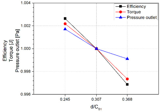
Figure 15.
Variation in the total-to-total efficiency, torque, and pressure outlet with changes in the axial gap for the three cases.
4. Conclusions
Herein, we presented a numerical study on the unsteady state to understand how turbine blades and their passages are affected by changes in the AG between the stator and rotor of a GE-E3 two-stage gas turbine that has a HS inlet temperature distribution. A turbulence model was used to examine the flow fields, heat flux, temperature, and other parameters, at the walls and the passage. In this process, the results were examined for 80% (case 1) and 120% (case 3) of the designed value for the AG of case 2 (13 mm or d/Cs1 = 0.307).
The results showed that the blade surface’s maximum temperature increased by over 110 K for the HS inlet conditions compared to uniform conditions. Therefore, an HS must be applied to clearly understand the turbine’s thermal characteristics. When the HS inlet conditions were applied, the results according to the AG showed that when the AG was reduced from case 3 to case 1, the surface suction side streamline of first stage rotor (R1) and second-stage rotor (R2) become closer to the endwall because of the secondary flow. Thus, it was formed in the radially outward direction at R1’s trailing edge. The area-averaged and maximum temperatures in R1 surface increased by 1.5 K and 3 K, respectively, and the area-averaged and maximum pressure increased by 2000 Pa and 400 Pa, respectively. The low temperature region near the tip and hub decreased. In the second-stage stator and R2, the area-averaged heat fluxes increased by 10.6% and 2.8%, respectively. As the AG decreased, the turbine overall efficiencies increased by 0.306% and 0.295%, respectively; however, this increases the blade surface’s thermal load and reduces the turbine blade fatigue life. If an appropriate cooling technology is developed, it will lead to the development of a higher efficiency design using a shorter AG and reduce long-term operating costs.
The unsteady RANS model used in this study has a low computational cost; however, it has the drawback of being unable to precisely predict vortices and flow separation phenomena that occur around the tips and walls. DES is more accurate; however, it has a high computational cost and previous studies using DES have mostly focused on the local flow phenomena rather than full blade simulations [25,26,27]. With significant advances in computational resources, it is expected that DES or LES will soon be used to accurately predict the complex unsteady flow physics near the tips and walls within full blade simulations.
Author Contributions
Conceptualization, methodology, investigation: M.G.C. and J.R.; validation, formal analysis, writing—original draft preparation, visualization: M.G.C.; writing—review and editing, supervision, project administration, funding acquisition: J.R.
Funding
This research was funded by Basic Science Research Program through the National Research Foundation of Korea (NRF-2017R1C1B2012068). Also, this research was funded by the Chung-Ang University Research Grants in 2017.
Conflicts of Interest
The authors declare no conflict of interest.
Nomenclature
| CS1 | Axial chord length of S1 [mm] |
| d | Axial chord length [mm] |
| Heat flux [W/m2] | |
| Wall temperature [K] | |
| Adiabatic wall temperature [K] | |
| Pressure [Pa] | |
| Inlet total pressure [Pa] | |
| Temperature [K] | |
| Inlet total temperature [K] | |
| X, Y, Z | Cartesian coordinates |
Abbreviations
| HP | High pressure |
| HS | Hot streak |
| S1, R1, S2, R2 | first stage stator, rotor, second-stage stator, rotor |
| HTC, h | Heat transfer coefficient |
| AG | Axial gap |
| LE | Leading edge |
| TE | Trailing edge |
| PS | Pressure side |
| SS | Suction side |
| AC, Ca | Axial chord |
| Subscripts | |
| ave | Averaged |
| max | Maximum value |
| min | Minimum value |
References
- Wang, Z.; Liu, Z.; Feng, Z. Influence of mainstream turbulence intensity on heat transfer characteristics of a high pressure turbine stage with inlet hot streak. J. Turbomach. 2016, 138, 041005. [Google Scholar] [CrossRef]
- Butler, T.L.; Sharma, O.P.; Dring, R.P. Redistribution of an inlet temperature distortion in an axial flow turbine stage. J. Propuls. Power 1989, 5, 64–71. [Google Scholar] [CrossRef]
- Povey, T.; Qureshi, I. A hot-streak (combustor) simulator suited to aerodynamic performance measurements. Proc. Inst. Mech. Eng. Part G J. Aerosp. Eng. 2008, 222, 705–720. [Google Scholar] [CrossRef]
- Gundy-Burlet, K.L.; Dorney, D.J. Effects of radial location on the migration of hot streaks in a turbine. J. Propuls. Power 2000, 16, 377–387. [Google Scholar] [CrossRef]
- An, B.T.; Liu, J.J.; Jiang, H.D. Numerical investigation on unsteady effects of hot streak on flow and heat transfer in a turbine stage. In Proceedings of the ASME Turbo Expo 2008: Power for Land, Sea, and Air, Berlin, Germany, 9–13 June 2008. [Google Scholar]
- Feng, Z.; Liu, Z.; Shi, Y.; Wang, Z. Effects of hot streak and airfoil clocking on heat transfer and aerodynamic characteristics in gas turbine. J. Turbomach. 2016, 138, 021002. [Google Scholar] [CrossRef]
- Smith, C.I.; Chang, D.; Tavoularis, S. Effect of inlet temperature nonuniformity on high-pressure turbine performance. In Proceedings of the ASME Turbo Expo 2010: Power for Land, Sea, and Air, Glasgow, UK, 14–18 June 2010. [Google Scholar]
- Yamada, K.; Funazaki, K.; Kikuchi, M.; Sato, H. Influences of axial gap between blade rows on secondary flow and aerodynamic performance in a turbine stage. In Proceedings of the ASME Turbo Expo 2009: Power for Land, Sea, and Air, Orlando, FL, USA, 8–12 June 2009. [Google Scholar]
- Danish, S.N.; Qureshi, S.R.; Imran, M.M.; Khan, S.U.; Sarfraz, M.M.; El-Leathy, A.; Al-Ansary, H.; Wei, M. Effect of tip clearance and rotor–stator axial gap on the efficiency of a multistage compressor. Appl. Therm. Eng. 2016, 99, 988–995. [Google Scholar] [CrossRef]
- Dring, R.P.; Joslyn, H.D.; Hardin, L.W.; Wagner, J.H. Turbine rotor-stator interaction. J. Eng. Power 1982, 104, 729–742. [Google Scholar] [CrossRef]
- Gaetani, P.; Persico, G.; Dossena, V.; Osnaghi, C. Investigation of the flow field in a HP turbine stage for two stator-rotor axial gaps: Part I—3D time averaged flow field. In Proceedings of the ASME Turbo Expo 2006: Power for Land, Sea and Air, Barcelona, Spain, 8–11 May 2006. [Google Scholar]
- Funazaki, K.I.; Yamada, K.; Kikuchi, M.; Sato, H. Experimental studies on aerodynamic performance and unsteady flow behaviors of a single turbine stage with variable rotor-stator axial gap: Comparisons with time-accurate numerical simulation. In Proceedings of the ASME Turbo Expo 2007: Power for Land, Sea, and Air, Montreal, QC, Canada, 14–17 May 2007. [Google Scholar]
- Sasao, Y.; Kato, H.; Yamamoto, S.; Satsuki, H.; Ooyama, H.; Ishizaka, K. Numerical and experimental investigations of unsteady 3-D flow through two-stage cascades in steam turbine model. In Proceedings of the International Conference on Power Engineering, Kobe, Japan, 16–20 November 2009. [Google Scholar]
- Ghenaiet, A.; Touil, K. Characterization of component interactions in two-stage axial turbine. Chin. J. Aeronaut. 2016, 29, 893–913. [Google Scholar] [CrossRef]
- Timko, L.P. Energy Efficient Engine High Pressure Turbine Component Test Performance Report; Technical Report; National Aeronautics and Space Administration (NASA): Cincinnati, OH, USA, 1 January 1984.
- Arnone, A.; Benvenuti, E. Three-dimensional Navier-Stokes analysis of a two-stage gas turbine. In Proceedings of the ASME 1994 International Gas Turbine and Aeroengine Congress and Exposition, The Hague, The Neterlands, 13–16 June 1994. [Google Scholar]
- Ryu, J.; Livescu, D. Turbulence structure behind the shock in canonical shock–vortical turbulence interaction. J. Fluid Mech. 2014, 756, R1. [Google Scholar] [CrossRef]
- Ryu, J.; Lele, S.K.; Viswanathan, K. Study of supersonic wave components in high-speed turbulent jets using an LES database. J. Sound Vib. 2014, 333, 6900–6923. [Google Scholar] [CrossRef]
- Celik, I.; Yavuz, I.; Smirnov, A. Large eddy simulations of in-cylinder turbulence for internal combustion engines: A review. Int. J. Engine Res. 2001, 2, 119–148. [Google Scholar] [CrossRef]
- Meloni, R.; Naso, V. An insight into the effect of advanced injection strategies on pollutant emissions of a heavy-duty diesel engine. Energies 2013, 6, 4331–4351. [Google Scholar] [CrossRef]
- Haworth, D.C.; Jansen, K. Large-eddy simulation on unstructured deforming meshes: Towards reciprocating IC engines. Comput. Fluids 2000, 29, 493–524. [Google Scholar] [CrossRef]
- Hao, Z.R.; Gu, C.W.; Ren, X.D. The application of discontinuous Galerkin methods in conjugate heat transfer simulations of gas turbines. Energies 2014, 7, 7857–7877. [Google Scholar] [CrossRef]
- Kim, J.; Park, J.G.; Kang, Y.S.; Cho, L.; Cho, J. A study on the numerical analysis methodology for thermal and flow characteristics of high pressure turbine in aircraft gas turbine engine. Korean Soc. Fluid Mach. 2013, 17, 46–51. [Google Scholar] [CrossRef]
- Hylton, L.; Mihelc, M.; Turner, E.; Nealy, D.; York, R. Analytical and Experimental Evaluation of the Heat Transfer Distribution over the Surfaces of Turbine Vanes; Technical Report; National Aeronautics and Space Administration (NASA): Indianapolis, IN, USA, 1 May 1983.
- Martini, P.; Schulz, A.; Bauer, H.J.; Whitney, C.F. Detached eddy simulation of film cooling performance on the trailing edge cutback of gas turbine airfoils. In Proceedings of the ASME Turbo Expo 2005: Power for Land, Sea, and Air, Reno, NV, USA, 6–9 June 2005. [Google Scholar]
- Effendy, M.; Yao, Y.F.; Yao, J.; Marchant, D.R. DES study of blade trailing edge cutback cooling performance with various lip thicknesses. Appl. Therm. Eng. 2016, 99, 434–445. [Google Scholar] [CrossRef]
- Mao, X.; Dal Monte, A.; Benini, E.; Zheng, Y. Numerical study on the internal flow field of a reversible turbine during continuous guide vane closing. Energies 2017, 10, 988. [Google Scholar] [CrossRef]


© 2018 by the authors. Licensee MDPI, Basel, Switzerland. This article is an open access article distributed under the terms and conditions of the Creative Commons Attribution (CC BY) license (http://creativecommons.org/licenses/by/4.0/).