Frequency-Adaptive Current Controller Design Based on LQR State Feedback Control for a Grid-Connected Inverter under Distorted Grid

Abstract

This paper proposes a frequency-adaptive current control design for a grid-connected inverter with an inductive–capacitive–inductive (LCL) filter to overcome the issues relating to both the harmonic distortion and frequency variation in the grid voltage. The current control scheme consists of full-state feedback control to stabilize the system and integral control terms to track the reference in the presence of disturbance and uncertainty. In addition, the current controller is augmented with resonant control terms to mitigate the harmonic component. The control scheme is implemented in the synchronous reference frame (SRF) to effectively compensate two harmonic orders at the same time by using only one resonant term. Moreover, to tackle the frequency variation issue in grid voltage, the frequency information which is extracted from the phase-locked loop (PLL) block is processed by a moving average filter (MAF) for the purpose of eliminating the frequency fluctuation caused by the harmonically distorted grid voltage. The filtered frequency information is employed to synthesize the resonant controller, even in the environment of frequency variation. To implement full-state feedback control for a grid-connected inverter with an LCL filter, all the state variables should be available. However, the increase in number of sensing devices leads to the rise of cost and complexity for hardware implementation. To overcome this challenge, a discrete-time full-state current observer is introduced to estimate all the system states. When the grid frequency is subject to variation, the discrete-time implementation of the observer in the SRF requires an online discretization process because the system matrix in the SRF includes frequency information. This results in a heavy computational burden for the controller. To resolve such a difficulty, a discrete-time observer in the stationary reference frame is employed in the proposed scheme. In the stationary frame, the discretization of the system model can be accomplished with a simple offline method even in the presence of frequency variation since the system matrix does not include the frequency. To select desirable gains for the full-state feedback controller and full-state observer, an optimal linear quadratic control approach is applied. To validate the practical effectiveness of the proposed frequency-adaptive control, simulation and experimental results are presented.

1. Introduction

Renewable energy systems (RESs) and distributed generation (DG) have been the subject of many studies in the last several years, and the growth in the utilization of DG to provide power to grid-connected inverters is also tangible. Generally, to mitigate pollution in the grid, the grid-connected inverter should possess high output power factor and low output current distortion [1]. In order to achieve this, a variety of current control schemes have been studied to produce injected current output to the grid that meets DG power quality standards such as the IEEE-519 in the USA or the IEC 61000-3-2 in Europe [2].

Several current control methods such as repetitive controllers, resonant controllers, and grid voltage feedforward controllers have been studied to reject the current harmonics. A repetitive controller presented in reference [3] can compensate the total harmonic distortion (THD) and yield zero steady-state tracking error due to the high gains at the fundamental and harmonic frequencies. Meanwhile, a linear current control scheme in reference [4] was constructed by series configuration of the tracking regulator and harmonic compensator for a single-phase grid-connected inverter. In this method, the harmonic compensator was designed by using several bandpass filters to eliminate the selected harmonic components. Aside from the previous approaches, resonant controllers have been widely studied both in the stationary reference frame [5,6,7] and in the synchronous reference frame (SRF) [8]. In general, to avoid the degradation of control performance in a resonant controller, exact knowledge of the frequency information should be required for adjustment of the resonant frequency in the case of grid frequency change. In addition, a different approach is presented in reference [9], in which the harmonic values of injected grid currents was mitigated by full feedforward control of grid voltages constructed with one proportional term and two derivative terms.

In tackling the current harmonic issue in power systems, the variation of grid frequency might cause a degradation of the control performance. Thus, frequency-adaptive control for a grid-connected inverter has motivated many studies to investigate a systematic design method for ensuring the high quality of injected grid currents, even under unexpected circumstances. In particular, an improved repetitive control (RC) scheme based on a finite impulse response (FIR) filter presented in reference [1] can be used to adjust the resonant frequencies of the controller according to the grid frequency to match them with the fundamental and harmonic frequencies of the grid. However, the dynamic response of RC is slower when compared with a feedback controller such as a proportional-integral (PI) or proportional-resonant (PR) controller. On the other hand, in the control scheme studied in reference [10], the frequency-adaptive task was realized with a second-order infinite impulse response (IIR) resonator with an online tuning algorithm. In reference [11], a selective harmonic control (SHC) was designed in the z domain to mitigate the harmonics from a distorted grid environment. Moreover, to cope with the frequency variation problem with a fixed sampling rate, the fractional-order part in the controller was replaced by Lagrange-polynomial-based interpolation filters. However, this method requires more multiplications and summations to deal with the fractional-order delays. As another approach, a frequency-adaptive current control scheme based on reduced-order generalized integrators (ROGIs) was applied for a grid-connected inverter equipped with an inductive (L) filter [12]. In this method, the authors implemented several ROGIs to compensate specific frequency harmonics, and also proposed a frequency estimation algorithm to update the resonance frequency of ROGIs online in order to avoid quality degradation in the presence of frequency variation.

In reference [13], a frequency-adaptive current control was designed based on an advanced PR controller in the discrete-time domain for a grid-connected alternating current/direct current (AC/DC) converter. This method shows capability to adjust the parameters and to maintain the system stability for a wide range of frequencies. However, to ensure a negligible frequency deviation during the discretization of the PR controller transfer function through the bilinear transformation, this scheme uses the relatively high switching frequency of 20 kHz. To improve the estimation performance of the grid phase and frequency in the presence of voltage harmonics, the study in reference [14] proposed an adaptive digital control scheme for three-phase active power filtering comprising an enhanced SRF phase-locked loop (PLL). This research work demonstrates the improvement in grid phase and frequency estimation as well as in current control performance under adverse grid conditions by means of the online updating of resonance parameters. With the purpose of simplifying the controller structure, a frequency-adaptive resonant controller without the PLL was introduced in reference [15]. Since the reference current is directly generated from the grid voltage in this scheme, the current controller is synchronized to the grid without any synchronization unit. Furthermore, the second-order generalized integrator-based frequency-locked loop (FLL) is connected to the current controller in order to provide an estimated grid frequency in the main resonant controller and the harmonic compensator under the grid frequency variation.

With regard to the implementation of a full-state feedback controller, the availability of all the system states is required, which normally causes an increase in the number of needed sensors. The alternative to using additional sensing devices is to construct the observer for the estimation of all the observable system states by using the system input and output only. There are some standard observer types studied in the literature; these are the full-state predictive observer [16,17,18], reduced-order state observer [19], and the full-state current observer [20]. In reference [20], a discrete-time full-state current observer was proposed to estimate all the states of an inductive–capacitive–inductive (LCL)-filtered grid-connected inverter. In this work, the full-state current observer was proven to be superior compared with the predictive-type observer since all the estimated values were obtained based on the current measurement. With respect to the choice of the reference frame for implementing the observer, the system model of the three-phase grid-connected inverter with an LCL filter includes the cross-coupling terms of frequency in the SRF [17,20], while those terms could be omitted in the model in the stationary frame [21]. Due to this aspect, obtaining the discrete-time model for an LCL-filtered grid-connected inverter is not easy when the grid frequency is subject to variation. This limitation can be overcome by introducing the observer design into the stationary reference frame. In the stationary frame, discretization of the system model can be accomplished easily with a simple offline method, even in the situation of frequency variation, since the system matrix does not include the frequency.

The selection of a current control structure for an LCL-filtered grid-connected inverter is also considered as another important aspect to optimize the computational burden as well as to guarantee the control objectives. To deal with the multiple state variables in the LCL-filtered grid-connected inverter, the control structure based on a full-state feedback has been demonstrated to be a more convenient approach to stabilizing the system. Furthermore, the PI and PR controllers can be easily combined into the state-space by means of the internal model principle [22] and also into an augmented control structure as additional control terms [20]. However, such a multivariable design approach poses a challenge to select appropriate controller gains to stabilize the system and achieve good performance in steady and transient states. Several studies related to the gain selection of a full-state feedback controller augmented with multiple control terms are presented in [16,17,20,23,24,25,26] with different approaches. Particularly, the studies in [16,17] introduce a straightforward method using the pole placement technique to select the system gains. However, the number of gains is significantly increased in the complex system, which makes these methods less attractive due to the time-consuming process. In references [23,24,25], a method based on linear matrix inequalities (LMIs) is presented by using the stability condition of the augmented system in the Lyapunov sense to obtain controller gains. Also, a linear quadratic regulator (LQR) is implemented in [20] by optimizing the cost function. Those methods are known as optimal controls that can provide the controller gains in a systematic way.

This paper proposes a frequency-adaptive current controller design for a grid-connected inverter with an LCL filter based on the LQR state feedback control approach in the presence of both harmonic distortion and frequency variation in the grid voltage. In the proposed scheme, a discrete-time full-state current observer in the stationary reference frame is employed to estimate the grid-side currents, inverter-side currents, and capacitor voltages. In the stationary frame, the discretization of the system model can be done with a simple offline method, even in the presence of frequency variation, since the system matrix does not include the frequency. Meanwhile, the current controller is realized in the SRF by full-state feedback control after augmenting the control structure with the integral and resonant terms. While the integral terms contribute to eliminating the steady-state error in the output current, the resonant terms are employed to compensate two harmonic components in the 6th and 12th order in the SRF at the same time. To construct the resonant controller, accurate information on the frequency is essential. In general, however, the frequency extracted from the conventional PLL shows fluctuations under harmonically distorted grid voltage. To eliminate such a fluctuation in frequency, a moving average filter (MAF) is employed and the filtered frequency information is used to synthesize the resonant controllers. Due to the integral and resonant terms augmented into the system model, a number of feedback gains should be selected in the proposed scheme. To overcome this limitation, an LQR-based control approach is adopted to select the feedback gains in a straightforward way. By minimizing the cost function, the entire system can be designed such that the stability and robustness of system are guaranteed. To prove the robustness of the proposed control scheme further, the variation of grid impedance is considered as parameter uncertainty. To validate the effectiveness and usefulness of the proposed control scheme, simulations using PSIM software (version 9.1, Powersim, Rockville, MD, USA) and experiments using a digital signal processor (DSP) TMS320F28335 are performed by utilizing a three-phase 2 kVA prototype grid-connected inverter. The results show that reference tracking and harmonic compensation can be accomplished effectively by the proposed scheme, even under grid frequency change, by using only the grid-side current sensors and grid voltage sensors.

This paper is organized as follows. Section 2 describes the system model of a grid-connected inverter with an LCL filter. Section 3 presents the proposed frequency-adaptive current control scheme. Section 4 and Section 5 present the simulation and experimental results, respectively. Finally, Section 6 concludes the paper.

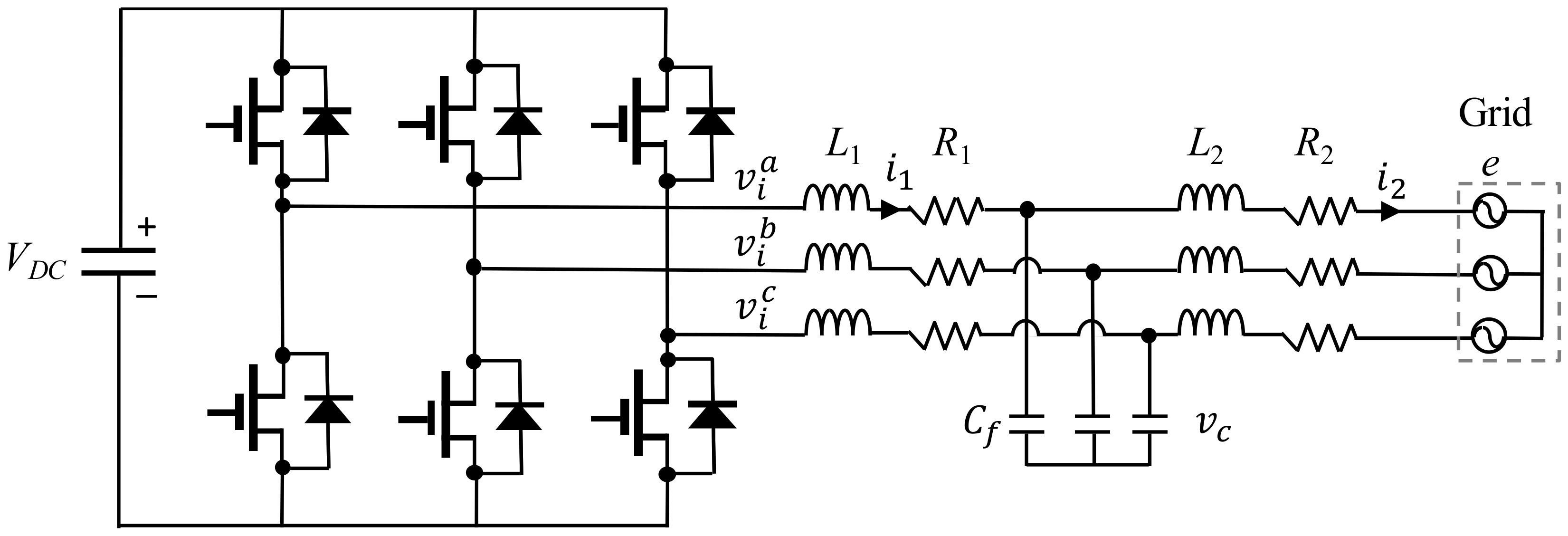
2. System Model of an LCL-Filtered Grid-Connected Inverter

2.1. Modeling of a Grid-Connected Inverter in the Synchronous Reference Frame

Whereas the SRF is used for the current controller design, the stationary reference frame is used for the design of the state observer. The three phase variables “$abc$” are transformed into the variables “$dq$” in the SRF by means of Park’s transformation as follows:

$$\left[\begin{array}{c}{f}^q\\ f^d\end{array}\right]=\frac{2}{3}\left[\begin{array}{c}\cos \left(\theta \right) \cos \left(\theta -\frac{2\pi }{3}\right) \cos \left(\theta +\frac{2\pi }{3}\right)\\ \sin \left(\theta \right) \sin \left(\theta -\frac{2\pi }{3}\right) \sin \left(\theta +\frac{2\pi }{3}\right)\end{array}\right]\left[\begin{array}{c}{f}^a\\ f^b\\ f^c\end{array}\right]$$

(1)

where $f$ denotes the variable being transformed and $\theta$ is the phase angle.

Figure 1 represents a configuration of the three-phase grid-connected inverter connected to the grid through an LCL filter, in which $V_{DC}$ represents the DC link voltage, $R_1$ and $R_2$ are the filter resistances, $L_1$ and $L_2$ are the filter inductances, and $C_f$ is the filter capacitance. The state equations of a grid-connected inverter are expressed in the SRF as follows:

$$\dot{i_2^q }=-\frac{R_2}{L_2}{i}_2^q-\omega i_2^d+\frac{1}{L_2}{v}_c^q-\frac{1}{L_2}{e}^q$$

(2)

$$\dot{i_2^d}=-\frac{R_2}{L_2}{i}_2^d+\omega i_2^q+\frac{1}{L_2}{v}_c^d-\frac{1}{L_2}{e}^d$$

(3)

$$\dot{i_1^q}=-\frac{R_1}{L_1}{i}_1^q-\omega i_1^d-\frac{1}{L_1}{v}_c^q+\frac{1}{L_1}{v}_i^q$$

(4)

$$\dot{i_1^d}=-\frac{R_1}{L_1}{i}_1^d+\omega i_1^q-\frac{1}{L_1}{v}_c^d+\frac{1}{L_1}{v}_i^d$$

(5)

$$\dot{v_c^q}=-\omega v_c^d-\frac{1}{C_f}{i}_2^q+\frac{1}{C_f}{i}_1^q$$

(6)

$$\dot{v_c^d}=\omega v_c^q-\frac{1}{C_f}{i}_2^d+\frac{1}{C_f}{i}_1^d$$

(7)

where the superscripts “q” and “d” denote the q-axis and d-axis variables on the SRF, respectively. In addition, $i_1$ is the inverter-side current, $i_2$ is the grid-side current, $v_c$ is the capacitor voltage, $e$ is the grid voltage, $v_i$ is the inverter output voltage, and $\omega$ is the angular frequency of the grid voltage.

From Equations (2) to (7), the continuous-time state-space model of the inverter system is expressed in the SRF as follows:

$${\dot{x}}_s\left(t\right)=A_s{x}_s\left(t\right)+B{u}_s\left(t\right)+D{e}_s\left(t\right)$$

(8)

$$y_s\left(t\right)=C{x}_s\left(t\right)$$

(9)

where $x_s={\left[i_2^q i_2^d i_1^q i_1^d v_c^q v_c^d \right]}^T$ is the system state vector, $u_s={\left[v_i^q v_i^d\right]}^T$ is the system input vector, $e_s={\left[e^q e^d\right]}^T$ is the grid voltage vector, and the system matrices $A_s$, $B$, $C$, and $D$ are expressed as

$$A_S=\left[\begin{array}{l}-R_2/L_2\hspace{0.17em}\hspace{0.17em}\hspace{0.17em}\hspace{0.17em}\hspace{0.17em}\hspace{0.17em}\hspace{0.17em}\hspace{0.17em}\hspace{0.17em}\hspace{0.17em}-\omega \hspace{0.17em}\hspace{0.17em}\hspace{0.17em}\hspace{0.17em}\hspace{0.17em}\hspace{0.17em}\hspace{0.17em}\hspace{0.17em}\hspace{0.17em}\hspace{0.17em}\hspace{0.17em}\hspace{0.17em}0\hspace{0.17em}\hspace{0.17em}\hspace{0.17em}\hspace{0.17em}\hspace{0.17em}\hspace{0.17em}\hspace{0.17em}\hspace{0.17em}\hspace{0.17em}\hspace{0.17em}\hspace{0.17em}\hspace{0.17em}\hspace{0.17em}\hspace{0.17em}\hspace{0.17em}\hspace{0.17em}0\hspace{0.17em}\hspace{0.17em}\hspace{0.17em}\hspace{0.17em}\hspace{0.17em}\hspace{0.17em}\hspace{0.17em}\hspace{0.17em}\hspace{0.17em}\hspace{0.17em}\hspace{0.17em}\hspace{0.17em}1/L_2\hspace{0.17em}\hspace{0.17em}\hspace{0.17em}\hspace{0.17em}\hspace{0.17em}\hspace{0.17em}\hspace{0.17em}\hspace{0.17em}0\hspace{0.17em}\\ \hspace{0.17em}\hspace{0.17em}\hspace{0.17em}\hspace{0.17em}\hspace{0.17em}\omega \hspace{0.17em}\hspace{0.17em}\hspace{0.17em}\hspace{0.17em}\hspace{0.17em}\hspace{0.17em}\hspace{0.17em}\hspace{0.17em}\hspace{0.17em}\hspace{0.17em}\hspace{0.17em}-R_2/L_2\hspace{0.17em}\hspace{0.17em}\hspace{0.17em}\hspace{0.17em}\hspace{0.17em}\hspace{0.17em}\hspace{0.17em}\hspace{0.17em}0\hspace{0.17em}\hspace{0.17em}\hspace{0.17em}\hspace{0.17em}\hspace{0.17em}\hspace{0.17em}\hspace{0.17em}\hspace{0.17em}\hspace{0.17em}\hspace{0.17em}\hspace{0.17em}\hspace{0.17em}\hspace{0.17em}\hspace{0.17em}\hspace{0.17em}\hspace{0.17em}0\hspace{0.17em}\hspace{0.17em}\hspace{0.17em}\hspace{0.17em}\hspace{0.17em}\hspace{0.17em}\hspace{0.17em}\hspace{0.17em}\hspace{0.17em}\hspace{0.17em}\hspace{0.17em}\hspace{0.17em}\hspace{0.17em}\hspace{0.17em}0\hspace{0.17em}\hspace{0.17em}\hspace{0.17em}\hspace{0.17em}\hspace{0.17em}\hspace{0.17em}\hspace{0.17em}\hspace{0.17em}\hspace{0.17em}\hspace{0.17em}1/L_2\\ \hspace{0.17em}\hspace{0.17em}\hspace{0.17em}\hspace{0.17em}\hspace{0.17em}0\hspace{0.17em}\hspace{0.17em}\hspace{0.17em}\hspace{0.17em}\hspace{0.17em}\hspace{0.17em}\hspace{0.17em}\hspace{0.17em}\hspace{0.17em}\hspace{0.17em}\hspace{0.17em}\hspace{0.17em}\hspace{0.17em}\hspace{0.17em}\hspace{0.17em}\hspace{0.17em}\hspace{0.17em}0\hspace{0.17em}\hspace{0.17em}\hspace{0.17em}\hspace{0.17em}\hspace{0.17em}\hspace{0.17em}\hspace{0.17em}\hspace{0.17em}-R_1/L_1\hspace{0.17em}\hspace{0.17em}\hspace{0.17em}\hspace{0.17em}\hspace{0.17em}\hspace{0.17em}\hspace{0.17em}\hspace{0.17em}\hspace{0.17em}-\omega \hspace{0.17em}\hspace{0.17em}\hspace{0.17em}\hspace{0.17em}\hspace{0.17em}\hspace{0.17em}\hspace{0.17em}\hspace{0.17em}\hspace{0.17em}-1/L_1\hspace{0.17em}\hspace{0.17em}\hspace{0.17em}\hspace{0.17em}\hspace{0.17em}\hspace{0.17em}\hspace{0.17em}\hspace{0.17em}0\\ \hspace{0.17em}\hspace{0.17em}\hspace{0.17em}\hspace{0.17em}\hspace{0.17em}0\hspace{0.17em}\hspace{0.17em}\hspace{0.17em}\hspace{0.17em}\hspace{0.17em}\hspace{0.17em}\hspace{0.17em}\hspace{0.17em}\hspace{0.17em}\hspace{0.17em}\hspace{0.17em}\hspace{0.17em}\hspace{0.17em}\hspace{0.17em}\hspace{0.17em}\hspace{0.17em}\hspace{0.17em}0\hspace{0.17em}\hspace{0.17em}\hspace{0.17em}\hspace{0.17em}\hspace{0.17em}\hspace{0.17em}\hspace{0.17em}\hspace{0.17em}\hspace{0.17em}\hspace{0.17em}\hspace{0.17em}\hspace{0.17em}\hspace{0.17em}\omega \hspace{0.17em}\hspace{0.17em}\hspace{0.17em}\hspace{0.17em}\hspace{0.17em}\hspace{0.17em}\hspace{0.17em}\hspace{0.17em}\hspace{0.17em}\hspace{0.17em}-R_1/L_1\hspace{0.17em}\hspace{0.17em}\hspace{0.17em}\hspace{0.17em}\hspace{0.17em}\hspace{0.17em}\hspace{0.17em}\hspace{0.17em}\hspace{0.17em}0\hspace{0.17em}\hspace{0.17em}\hspace{0.17em}\hspace{0.17em}\hspace{0.17em}\hspace{0.17em}\hspace{0.17em}\hspace{0.17em}\hspace{0.17em}-1/L_1\\ \hspace{0.17em}-1/C_f\hspace{0.17em}\hspace{0.17em}\hspace{0.17em}\hspace{0.17em}\hspace{0.17em}\hspace{0.17em}\hspace{0.17em}\hspace{0.17em}\hspace{0.17em}\hspace{0.17em}\hspace{0.17em}\hspace{0.17em}\hspace{0.17em}0\hspace{0.17em}\hspace{0.17em}\hspace{0.17em}\hspace{0.17em}\hspace{0.17em}\hspace{0.17em}\hspace{0.17em}\hspace{0.17em}\hspace{0.17em}\hspace{0.17em}\hspace{0.17em}1/C_f\hspace{0.17em}\hspace{0.17em}\hspace{0.17em}\hspace{0.17em}\hspace{0.17em}\hspace{0.17em}\hspace{0.17em}\hspace{0.17em}\hspace{0.17em}\hspace{0.17em}\hspace{0.17em}\hspace{0.17em}0\hspace{0.17em}\hspace{0.17em}\hspace{0.17em}\hspace{0.17em}\hspace{0.17em}\hspace{0.17em}\hspace{0.17em}\hspace{0.17em}\hspace{0.17em}\hspace{0.17em}\hspace{0.17em}\hspace{0.17em}\hspace{0.17em}\hspace{0.17em}\hspace{0.17em}0\hspace{0.17em}\hspace{0.17em}\hspace{0.17em}\hspace{0.17em}\hspace{0.17em}\hspace{0.17em}\hspace{0.17em}\hspace{0.17em}\hspace{0.17em}-\omega \\ \hspace{0.17em}\hspace{0.17em}\hspace{0.17em}\hspace{0.17em}\hspace{0.17em}0\hspace{0.17em}\hspace{0.17em}\hspace{0.17em}\hspace{0.17em}\hspace{0.17em}\hspace{0.17em}\hspace{0.17em}\hspace{0.17em}\hspace{0.17em}\hspace{0.17em}\hspace{0.17em}\hspace{0.17em}\hspace{0.17em}-1/C_f\hspace{0.17em}\hspace{0.17em}\hspace{0.17em}\hspace{0.17em}\hspace{0.17em}\hspace{0.17em}\hspace{0.17em}\hspace{0.17em}\hspace{0.17em}0\hspace{0.17em}\hspace{0.17em}\hspace{0.17em}\hspace{0.17em}\hspace{0.17em}\hspace{0.17em}\hspace{0.17em}\hspace{0.17em}\hspace{0.17em}\hspace{0.17em}\hspace{0.17em}\hspace{0.17em}\hspace{0.17em}\hspace{0.17em}1/C_f\hspace{0.17em}\hspace{0.17em}\hspace{0.17em}\hspace{0.17em}\hspace{0.17em}\hspace{0.17em}\hspace{0.17em}\hspace{0.17em}\hspace{0.17em}\hspace{0.17em}\omega \hspace{0.17em}\hspace{0.17em}\hspace{0.17em}\hspace{0.17em}\hspace{0.17em}\hspace{0.17em}\hspace{0.17em}\hspace{0.17em}\hspace{0.17em}\hspace{0.17em}\hspace{0.17em}0\end{array}\right]$$

(10)

$$B=\left[\begin{array}{cc}\begin{array}{c}0\\ 0\\ 1/L_1\end{array}& \begin{array}{c}0\\ 0\\ 0\end{array}\\ \begin{array}{c}0\\ 0\\ 0\end{array}& \begin{array}{c}1/L_1\\ 0\\ 0\end{array}\end{array}\right], D=\left[\begin{array}{cc}\begin{array}{c}-1/L_2\\ 0\\ 0\end{array}& \begin{array}{c}0\\ -1/L_2\\ 0\end{array}\\ \begin{array}{c}0\\ 0\\ 0\end{array}& \begin{array}{c}0\\ 0\\ 0\end{array}\end{array}\right], C =\left[\begin{array}{cc}\begin{array}{c}\begin{array}{ccc}1& 0& 0\end{array}\\ \begin{array}{ccc}0& 1& 0\end{array}\end{array}& \begin{array}{c}\begin{array}{ccc}0& 0& 0\end{array}\\ \begin{array}{ccc}0& 0& 0\end{array}\end{array}\end{array}\right]$$

(11)

2.2. Discretization of the System Model

A discrete-time model is necessary for a digital implementation. The system model in Equations (8) and (9) is discretized using the zero-order hold (ZOH) with the sampling time $T_s$. as follows [27]:

$$x_s\left(k+1\right)=A_{sd}{x}_s\left(k\right)+B_{sd}{u}_s\left(k\right)+D_{sd}{e}_s$$

(12)

$$y_s\left(k\right)=C_{sd}{x}_s\left(k\right)$$

(13)

where the matrices $A_{sd}$, $B_{sd}$, $C_{sd}$, and $D_{sd}$ can be obtained as follows:

$$A_{sd}=e^{A_s{T}_s}$$

(14)

$$B_{sd}=\left({{\displaystyle \int }}_0^{T_s}{e}^{A_s{T}_s}dt\right)B, C_{sd}=C$$

(15)

$$D_{sd}=\left({{\displaystyle \int }}_0^{T_s}{e}^{A_s{T}_s}dt\right)D .$$

(16)

3. Proposed Frequency-Adaptive Current Control Scheme

Figure 2 represents the proposed frequency-adaptive current control scheme for a three-phase grid-connected inverter with an LCL filter. The PLL block generates the phase angle of the grid voltage to synchronize the grid-connected inverter with the grid. To reduce the fluctuation in frequency under harmonically distorted grid conditions, the frequency information extracted from the PLL block is filtered by the MAF to obtain $\tilde{\omega }$. The proposed frequency-adaptive control design consists of an integral-resonant state feedback controller in the SRF and a full-state current observer in the stationary reference frame in which both schemes are built in the discrete-time domain. The full-state current observer is constructed to estimate the system states $x_s$ from the control input $u_s$ and system output $y_s$. The estimated states are used to implement the full-state feedback controller. While integral control is employed to track the reference without a steady-state error in output current, the resonant controls are introduced to mitigate the harmonic currents. To accurately constitute the resonant controllers which compensate two harmonic components in the 6th and 12th orders in the SRF, the output $\tilde{\omega }$ of the MAF is employed.

3.1. Frequency Detection under Distorted Grid Voltage

The frequency deviation in the grid voltage may affect the current control performance in a grid-connected inverter, especially in the resonant controllers for harmonic compensation, resulting in the degradation of the power quality of the DG system. To resolve the issue, a frequency-adaptive scheme is adopted in this paper. In the proposed scheme, an accurate frequency detection method based on the MAF is first presented to remove the fluctuation in frequency under a harmonically distorted grid environment, and then the design of the resonant controllers using detected frequency information is presented to mitigate the current harmonics. Figure 3 shows the frequency detection method of grid voltage based on the MAF. Frequency $\overline{\omega }$ obtained from the PLL has fluctuation due to the distorted grid voltage. In order to eliminate such fluctuation, $\overline{\omega }$ is filtered by the MAF to determine the fundamental grid frequency $\tilde{\omega }$ [23,28].

3.2. Optimal Feedback Current Control Design Based on IM

The integral-resonant state feedback control is designed to guarantee both a zero tracking error for references and harmonic compensation for the 6th and 12th orders in the SRF by augmenting system model with integral and resonant terms in the discrete-time state-space. An integral term is expressed in the discrete-time state-space as [10]

$$\left[\begin{array}{c}{x}_i^q\left(k+1\right)\\ x_i^d\left(k+1\right)\end{array}\right]=G\left[\begin{array}{c}{x}_i^q\left(k\right)\\ x_i^d\left(k\right)\end{array}\right]+H\left[\begin{array}{c}{\epsilon }^q\left(k\right)\\ {\epsilon }^d\left(k\right)\end{array}\right]$$

(17)

where $\epsilon ={\left[{\epsilon }^q {\epsilon }^d\right]}^T=r- C_{sd}{x}_s$ is the current error vector, $r={\left[i_2^{q*} i_2^{d*}\right]}^T$ is the reference current vector, $G= \left[\begin{array}{cc}1& 0\\ 0& 1\end{array}\right]$, and $H=T_s\left[\begin{array}{cc}1& 0\\ 0& 1\end{array}\right]$.

In order to compensate the harmonic components in the 6th and 12th orders without performance degradation during the discretization process, discrete-time resonant terms are implemented directly by using the scheme in reference [29]. The transfer function of the resonant control in the s domain is expressed as

$$R_k\left(s\right)=\frac{s}{s^2+{\omega }_k^2}$$

(18)

where ${\omega }_k$ is the resonant angular frequency. Equation (18) is transformed by means of the pole–zero matching method [30] to obtain the transfer function in the z domain as follows:

$$R_k\left(z\right)=\frac{z^2-\cos \left({\omega }_k{T}_s\right)z}{z^2-2\cos \left({\omega }_k{T}_s\right)z+1} .$$

(19)

Considering the harmonic components in the 6th and 12th orders, Equation (19) can be expressed in the discrete-time state-space as

$$\left[\begin{array}{c}\begin{array}{c}{\delta }_{1j}^q\left(k+1\right)\\ {\delta }_{2j}^q\left(k+1\right)\end{array}\\ \begin{array}{c}{\delta }_{1j}^d\left(k+1\right)\\ {\delta }_{2j}^d\left(k+1\right)\end{array}\end{array}\right]=A_{rcj}\left[\begin{array}{c}\begin{array}{c}{\delta }_{1j}^q\left(k\right)\\ {\delta }_{2j}^q\left(k\right)\end{array}\\ \begin{array}{c}{\delta }_{1j}^d\left(k\right)\\ {\delta }_{2j}^d\left(k\right)\end{array}\end{array}\right]+B_{rcj}\left[\begin{array}{c}{\epsilon }^q\left(k\right)\\ {\epsilon }^d\left(k\right)\end{array}\right]\cdots \mathrm{for} j=6, 12$$

(20)

where

$$\begin{gathered} A_{rcj}= \left[\begin{array}{cc}\begin{array}{cc}2\cos \left(j{\omega }_k{T}_s\right)& 1\\ -1& 0\end{array}& \\ & \begin{array}{cc}2\cos \left(j{\omega }_k{T}_s\right)& 1\\ -1& 0\end{array}\end{array}\right] \\ B_{rcj}=\left[\begin{array}{cc}\begin{array}{c}\cos \left(j{\omega }_k{T}_s\right)\\ -1\end{array}& \\ & \begin{array}{c}\cos \left(j{\omega }_k{T}_s\right)\\ -1\end{array}\end{array}\right]. \end{gathered}$$

The integral and resonant terms in Equations (17) and (19) are augmented with

$$n_c\left(k+1\right)=\mathsf{\Phi }{n}_c\left(k\right)+\Gamma \epsilon \left(k\right)$$

(21)

where $n_c={\left[n_0 n_6 n_{12}\right]}^T$ is all state variables for integral and resonant terms with $n_0= {\left[x_i^q x_i^d\right]}^T$, $n_6={\left[{\delta }_{16 }^q{\delta }_{26}^q {\delta }_{16}^d {\delta }_{26}^d\right]}^T$, $n_{12}={\left[{\delta }_{112}^q {\delta }_{212}^q {\delta }_{112}^d {\delta }_{212}^d\right]}^T$,

$$\mathsf{\Phi }=\left[\begin{array}{ccc}G& & \\ & A_{rc6}& \\ & & A_{rc12}\end{array}\right] , \mathrm{and} \Gamma =\left[\begin{array}{c}H\\ B_{rc6}\\ B_{rc12}\end{array}\right].$$

By using Equations (12), (13), and (21), the entire control system can be combined into matrix form as follows:

$$\left[\begin{array}{c}{x}_s\left(k+1\right)\\ n_c\left(k+1\right)\end{array}\right]=\left[\begin{array}{cc}{A}_{sd}& 0\\ -\Gamma C_{sd}& \mathsf{\Phi }\end{array}\right]\left[\begin{array}{c}{x}_s\left(k\right)\\ n_c\left(k\right)\end{array}\right]+\left[\begin{array}{c}{B}_{sd}\\ 0\end{array}\right]u_s\left(k\right)+\left[\begin{array}{c}{D}_{sd}\\ 0\end{array}\right]e_s\left(k\right)+\left[\begin{array}{c}0\\ \Gamma \end{array}\right]r\left(k\right)$$

(22)

$$y_s\left(k\right)=\left[\begin{array}{cc}{C}_{sd}& 0\end{array}\right]\left[\begin{array}{c}{x}_s\left(k\right)\\ n_c\left(k\right)\end{array}\right].$$

(23)

Considering the augmented system, the state feedback control law can be obtained as

$$u_s\left(k\right)=-\left[K_x K_n\right]\left[\begin{array}{c}{x}_s\left(k\right)\\ n_c\left(k\right)\end{array}\right]=u_x\left(k\right)+u_n\left(k\right)$$

(24)

where $u_x\left(k\right)=-K_x{x}_s\left(k\right)$, $u_n\left(k\right)=-K_n{n}_c\left(k\right)$, $K_x$ represents the gain vector for the state feedback control, and $K_n$ denotes the gain vector for the integral and resonant controls.

The augmented system in Equations (22)–(24) can be rewritten in a compact form as

$$x_e\left(k+1\right)=A_e{x}_e\left(k\right)+B_e{u}_s\left(k\right)+D_e{e}_s\left(k\right)+B_{re}r\left(k\right)$$

(25)

$$y_s\left(k\right)=C_e{x}_e\left(k\right)$$

(26)

$$u_s\left(k\right)=-K{x}_e\left(k\right)$$

(27)

where $K=\left[K_x K_n\right]$ is a set of feedback gains and $K_n=\left[K_{no} K_{n6} K_{n12}\right]$, in which $K_{no}, K_{n6}, \mathrm{and} K_{n12}$ denote the gains for the integral terms and the resonant terms in the 6th and 12th orders, respectively.

To ensure the system stability and control performance, the state feedback control input $u_s\left(k\right)$ is designed using an optimal control method, in which the gain matrix $K$ in the system given by Equations (25)–(27) is evaluated systematically by minimizing the discrete quadratic cost function as follows [31,32]:

$$J=\frac{1}{2}{\displaystyle \sum }_{k=0}^{\infty }{x}_e{}^T\left(k\right)Q{x}_e\left(k\right)+u_s{}^T\left(k\right)R{u}_s\left(k\right)$$

(28)

where $Q$ is a positive semidefinite matrix and $R$ is a positive definite matrix. An $n\times n$ real symmetric matrix $P$ with $n$ being the number of state variables can be determined as the solution to the discrete algebraic Riccati equation (ARE) to obtain the optimal control input $u_s\left(k\right)$ in closed-loop form as

$$P=Q+A_e{}^{T}P{A}_e-A_e{}^{T}P{B}_e{\left(R+B_e{}^{T}P{B}_e\right)}^{-1}{B}_e{}^{T}P{A}_e .$$

(29)

The weighting matrices $Q$ and $R$ determine the relative importance of the state error and energy expenditure. The system behavior with regard to the selection of the weighting matrices $Q$ and $R$ has been analyzed in detail and the process of selecting the weighting matrices can be done by the trial and error method based on the characteristics of the system state and controller [20]. Also, choosing the weighting matrices $Q$ and $R$ can be accomplished according to the guideline presented for a voltage source converter in reference [33]. The discrete ARE in Equation (29) can be solved using the “dlqr” function in MATLAB. In this paper, the weighting matrices $Q$ and $R$. are selected to be

$$Q=\left[\begin{array}{cc}\begin{array}{c}{\mathbf{0}}^{6\times 6}\\ \begin{array}{c}{\mathbf{0}}^{2\times 6}\\ \begin{array}{c}{\mathbf{0}}^{4\times 6}\\ {\mathbf{0}}^{4\times 6}\end{array}\end{array}\end{array}& \begin{array}{cc}\begin{array}{c}{\mathbf{0}}^{6\times 2}\\ \begin{array}{c}{10}^{9.2}·I^{2\times 2}\\ \begin{array}{c}{\mathbf{0}}^{4\times 2}\\ {\mathbf{0}}^{4\times 2}\end{array}\end{array}\end{array}& \begin{array}{cc}\begin{array}{c}{\mathbf{0}}^{6\times 4}\\ \begin{array}{c}{\mathbf{0}}^{2\times 4}\\ \begin{array}{c}0.5·I^{4\times 4}\\ {\mathbf{0}}^{4\times 4}\end{array}\end{array}\end{array}& \begin{array}{c}{\mathbf{0}}^{6\times 4}\\ \begin{array}{c}{\mathbf{0}}^{2\times 4}\\ \begin{array}{c}{\mathbf{0}}^{4\times 4}\\ 0.03·I^{4\times 4}\end{array}\end{array}\end{array}\end{array}\end{array}\end{array}\right], R=\left[\begin{array}{cc}1& 0\\ 0& 1\end{array}\right]$$

(30)

where ${\mathbf{0}}^{n\times m}$ and $I^{n\times m}$ denote the zero and identity matrices with $n\times m$ dimension, respectively.

3.3. Design of the Discrete-Time Observer in the Stationary Reference Frame

Even though the implementation of a full-state feedback control requires all the system states to be accessible, the measurement of the system states by using additional sensing devices is not desirable since it leads to increases in cost and design complexity. Hence, an observer-based estimation is introduced in the proposed scheme to estimate the system states.

In view of the computational burden of the controller, offline discretization of the system model based on ZOH is often preferred. Another discretization scheme such as the forward Euler method does not map the stable region of the continuous-time system into that of the discrete-time system exactly, although it is simple to implement online [31]. However, the continuous-time model of the inverter system expressed in the SRF requires information on the angular frequency of the grid voltage in the system matrix. As a result, the continuous-time model in Equations (8) and (9) cannot be discretized simply by the offline ZOH method under frequency variation. Instead, the discretization should be done online with the frequency information in each sampling period. However, the implementation of online discretization based on the ZOH method is a heavy and complex task. In order to avoid this difficulty in the circumstance of frequency variation, a discrete-time full-state current observer is designed in the stationary reference frame. In the stationary frame, the inverter system can be discretized simply using the offline method because the system model does not include frequency information.

The system model for the LCL-filtered grid-connected inverter is expressed in the stationary reference frame as follows:

$$\dot{i_2^{\alpha } }=-\frac{R_2}{L_2}{i}_2^{\alpha }+\frac{1}{L_2}{v}_c^{\alpha }-\frac{1}{L_2}{e}^{\alpha }$$

(31)

$$\dot{i_2^{\beta }}=-\frac{R_2}{L_2}{i}_2^{\beta }+\frac{1}{L_2}{v}_c^{\beta }-\frac{1}{L_2}{e}^{\beta }$$

(32)

$$\dot{i_1^{\alpha }}=-\frac{R_1}{L_1}{i}_1^{\alpha }-\frac{1}{L_1}{v}_c^{\alpha }+\frac{1}{L_1}{v}_i^{\alpha }$$

(33)

$$\dot{i_1^{\beta }}=-\frac{R_1}{L_1}{i}_1^{\beta }-\frac{1}{L_1}{v}_c^{\beta }+\frac{1}{L_1}{v}_i^{\beta }$$

(34)

$$\dot{v_c^{\alpha }}=-\frac{1}{C_f}{i}_2^{\alpha }+\frac{1}{C_f}{i}_1^{\alpha }$$

(35)

$$\dot{v_c^{\beta }}=-\frac{1}{C_f}{i}_2^{\beta }+\frac{1}{C_f}{i}_1^{\beta }$$

(36)

where the superscripts “α” and “β” denote the variables in the stationary reference frame. From Equations (31) to (36), the continuous-time model is expressed in the state-space as

$$\dot{x}\left(t\right)=Ax\left(t\right)+Bu\left(t\right)+De\left(t\right)$$

(37)

$$y\left(t\right)=Cx\left(t\right)$$

(38)

where $x={\left[i_2^{\alpha } i_2^{\beta } i_1^{\alpha } i_1^{\beta } v_c^{\alpha } v_c^{\beta } \right]}^T$ is the system state vector, $u={\left[v_i^{\alpha } v_i^{\beta }\right]}^T$ is the system input vector, and $e={\left[e^{\alpha } e^{\beta }\right]}^T$ is the grid voltage vector. The system matrices $B$, $C$, and $D$ are defined the same as in Equation (11) and the matrix $A$ is expressed as

$$A_S=\left[\begin{array}{l}-R_2/L_2\hspace{0.17em}\hspace{0.17em}\hspace{0.17em}\hspace{0.17em}\hspace{0.17em}\hspace{0.17em}\hspace{0.17em}\hspace{0.17em}\hspace{0.17em}\hspace{0.17em}\hspace{0.17em}\hspace{0.17em}0\hspace{0.17em}\hspace{0.17em}\hspace{0.17em}\hspace{0.17em}\hspace{0.17em}\hspace{0.17em}\hspace{0.17em}\hspace{0.17em}\hspace{0.17em}\hspace{0.17em}\hspace{0.17em}\hspace{0.17em}0\hspace{0.17em}\hspace{0.17em}\hspace{0.17em}\hspace{0.17em}\hspace{0.17em}\hspace{0.17em}\hspace{0.17em}\hspace{0.17em}\hspace{0.17em}\hspace{0.17em}\hspace{0.17em}\hspace{0.17em}\hspace{0.17em}\hspace{0.17em}\hspace{0.17em}\hspace{0.17em}0\hspace{0.17em}\hspace{0.17em}\hspace{0.17em}\hspace{0.17em}\hspace{0.17em}\hspace{0.17em}\hspace{0.17em}\hspace{0.17em}\hspace{0.17em}\hspace{0.17em}\hspace{0.17em}\hspace{0.17em}1/L_2\hspace{0.17em}\hspace{0.17em}\hspace{0.17em}\hspace{0.17em}\hspace{0.17em}\hspace{0.17em}\hspace{0.17em}\hspace{0.17em}0\hspace{0.17em}\\ \hspace{0.17em}\hspace{0.17em}\hspace{0.17em}\hspace{0.17em}\hspace{0.17em}0\hspace{0.17em}\hspace{0.17em}\hspace{0.17em}\hspace{0.17em}\hspace{0.17em}\hspace{0.17em}\hspace{0.17em}\hspace{0.17em}\hspace{0.17em}\hspace{0.17em}\hspace{0.17em}-R_2/L_2\hspace{0.17em}\hspace{0.17em}\hspace{0.17em}\hspace{0.17em}\hspace{0.17em}\hspace{0.17em}\hspace{0.17em}\hspace{0.17em}0\hspace{0.17em}\hspace{0.17em}\hspace{0.17em}\hspace{0.17em}\hspace{0.17em}\hspace{0.17em}\hspace{0.17em}\hspace{0.17em}\hspace{0.17em}\hspace{0.17em}\hspace{0.17em}\hspace{0.17em}\hspace{0.17em}\hspace{0.17em}\hspace{0.17em}\hspace{0.17em}0\hspace{0.17em}\hspace{0.17em}\hspace{0.17em}\hspace{0.17em}\hspace{0.17em}\hspace{0.17em}\hspace{0.17em}\hspace{0.17em}\hspace{0.17em}\hspace{0.17em}\hspace{0.17em}\hspace{0.17em}\hspace{0.17em}\hspace{0.17em}0\hspace{0.17em}\hspace{0.17em}\hspace{0.17em}\hspace{0.17em}\hspace{0.17em}\hspace{0.17em}\hspace{0.17em}\hspace{0.17em}\hspace{0.17em}\hspace{0.17em}1/L_2\\ \hspace{0.17em}\hspace{0.17em}\hspace{0.17em}\hspace{0.17em}\hspace{0.17em}0\hspace{0.17em}\hspace{0.17em}\hspace{0.17em}\hspace{0.17em}\hspace{0.17em}\hspace{0.17em}\hspace{0.17em}\hspace{0.17em}\hspace{0.17em}\hspace{0.17em}\hspace{0.17em}\hspace{0.17em}\hspace{0.17em}\hspace{0.17em}\hspace{0.17em}\hspace{0.17em}\hspace{0.17em}0\hspace{0.17em}\hspace{0.17em}\hspace{0.17em}\hspace{0.17em}\hspace{0.17em}\hspace{0.17em}\hspace{0.17em}\hspace{0.17em}-R_1/L_1\hspace{0.17em}\hspace{0.17em}\hspace{0.17em}\hspace{0.17em}\hspace{0.17em}\hspace{0.17em}\hspace{0.17em}\hspace{0.17em}\hspace{0.17em}\hspace{0.17em}0\hspace{0.17em}\hspace{0.17em}\hspace{0.17em}\hspace{0.17em}\hspace{0.17em}\hspace{0.17em}\hspace{0.17em}\hspace{0.17em}\hspace{0.17em}\hspace{0.17em}-1/L_1\hspace{0.17em}\hspace{0.17em}\hspace{0.17em}\hspace{0.17em}\hspace{0.17em}\hspace{0.17em}\hspace{0.17em}\hspace{0.17em}0\\ \hspace{0.17em}\hspace{0.17em}\hspace{0.17em}\hspace{0.17em}\hspace{0.17em}0\hspace{0.17em}\hspace{0.17em}\hspace{0.17em}\hspace{0.17em}\hspace{0.17em}\hspace{0.17em}\hspace{0.17em}\hspace{0.17em}\hspace{0.17em}\hspace{0.17em}\hspace{0.17em}\hspace{0.17em}\hspace{0.17em}\hspace{0.17em}\hspace{0.17em}\hspace{0.17em}\hspace{0.17em}0\hspace{0.17em}\hspace{0.17em}\hspace{0.17em}\hspace{0.17em}\hspace{0.17em}\hspace{0.17em}\hspace{0.17em}\hspace{0.17em}\hspace{0.17em}\hspace{0.17em}\hspace{0.17em}\hspace{0.17em}0\hspace{0.17em}\hspace{0.17em}\hspace{0.17em}\hspace{0.17em}\hspace{0.17em}\hspace{0.17em}\hspace{0.17em}\hspace{0.17em}\hspace{0.17em}\hspace{0.17em}-R_1/L_1\hspace{0.17em}\hspace{0.17em}\hspace{0.17em}\hspace{0.17em}\hspace{0.17em}\hspace{0.17em}\hspace{0.17em}\hspace{0.17em}\hspace{0.17em}\hspace{0.17em}0\hspace{0.17em}\hspace{0.17em}\hspace{0.17em}\hspace{0.17em}\hspace{0.17em}\hspace{0.17em}\hspace{0.17em}\hspace{0.17em}-1/L_1\\ \hspace{0.17em}-1/C_f\hspace{0.17em}\hspace{0.17em}\hspace{0.17em}\hspace{0.17em}\hspace{0.17em}\hspace{0.17em}\hspace{0.17em}\hspace{0.17em}\hspace{0.17em}\hspace{0.17em}\hspace{0.17em}\hspace{0.17em}\hspace{0.17em}0\hspace{0.17em}\hspace{0.17em}\hspace{0.17em}\hspace{0.17em}\hspace{0.17em}\hspace{0.17em}\hspace{0.17em}\hspace{0.17em}\hspace{0.17em}\hspace{0.17em}\hspace{0.17em}1/C_f\hspace{0.17em}\hspace{0.17em}\hspace{0.17em}\hspace{0.17em}\hspace{0.17em}\hspace{0.17em}\hspace{0.17em}\hspace{0.17em}\hspace{0.17em}\hspace{0.17em}\hspace{0.17em}\hspace{0.17em}0\hspace{0.17em}\hspace{0.17em}\hspace{0.17em}\hspace{0.17em}\hspace{0.17em}\hspace{0.17em}\hspace{0.17em}\hspace{0.17em}\hspace{0.17em}\hspace{0.17em}\hspace{0.17em}\hspace{0.17em}\hspace{0.17em}\hspace{0.17em}0\hspace{0.17em}\hspace{0.17em}\hspace{0.17em}\hspace{0.17em}\hspace{0.17em}\hspace{0.17em}\hspace{0.17em}\hspace{0.17em}\hspace{0.17em}\hspace{0.17em}\hspace{0.17em}0\\ \hspace{0.17em}\hspace{0.17em}\hspace{0.17em}\hspace{0.17em}\hspace{0.17em}0\hspace{0.17em}\hspace{0.17em}\hspace{0.17em}\hspace{0.17em}\hspace{0.17em}\hspace{0.17em}\hspace{0.17em}\hspace{0.17em}\hspace{0.17em}\hspace{0.17em}\hspace{0.17em}\hspace{0.17em}\hspace{0.17em}-1/C_f\hspace{0.17em}\hspace{0.17em}\hspace{0.17em}\hspace{0.17em}\hspace{0.17em}\hspace{0.17em}\hspace{0.17em}\hspace{0.17em}\hspace{0.17em}0\hspace{0.17em}\hspace{0.17em}\hspace{0.17em}\hspace{0.17em}\hspace{0.17em}\hspace{0.17em}\hspace{0.17em}\hspace{0.17em}\hspace{0.17em}\hspace{0.17em}\hspace{0.17em}\hspace{0.17em}\hspace{0.17em}\hspace{0.17em}1/C_f\hspace{0.17em}\hspace{0.17em}\hspace{0.17em}\hspace{0.17em}\hspace{0.17em}\hspace{0.17em}\hspace{0.17em}\hspace{0.17em}\hspace{0.17em}\hspace{0.17em}0\hspace{0.17em}\hspace{0.17em}\hspace{0.17em}\hspace{0.17em}\hspace{0.17em}\hspace{0.17em}\hspace{0.17em}\hspace{0.17em}\hspace{0.17em}\hspace{0.17em}\hspace{0.17em}0\end{array}\right].$$

(39)

The system model in the stationary frame in Equations (37) and (38) is discretized similarly by using ZOH with the sampling time as follows [27]:

$$x\left(k+1\right)=A_{d}x\left(k\right)+B_{d}u\left(k\right)+D_{d}e\left(k\right)$$

(40)

$$y\left(k\right)=C_{d}x\left(k\right)$$

(41)

where the matrices $A_d$, $B_d$, $C_d$, and $D_d$ are calculated as

$$A_d=e^{A{T}_s}$$

(42)

$$B_d=\left({{\displaystyle \int }}_0^{T_s}{e}^{A{T}_s}dt\right)B, C_d=C$$

(43)

$$D_d=\left({{\displaystyle \int }}_0^{T_s}{e}^{A{T}_s}dt\right)D.$$

(44)

A detailed explanation regarding the full-state current observer and a comparison with the prediction-type observer and reduced-order observer are given in references [20,31]. Due to the advantage of the current-type observer over the prediction-type observer, the proposed scheme employs a full-state current observer to estimate the system states. From the discretized model of the inverter system in Equations (40) and (41), a discrete-time full-state current observer is constructed as follows:

$$\overline{x}\left(k+1\right)=A_d\widehat{x}\left(k\right)+B_{d}u\left(k\right)+D_{d}e\left(k\right)$$

(45)

$$\widehat{x}\left(k+1\right)=\overline{x}\left(k+1\right)+K_e\left[y\left(k+1\right)-C_d\overline{x}\left(k+1\right)\right]$$

(46)

where the symbol “^” denotes the estimated quantities, $K_e$ is the observer gain matrix, and $\overline{x}\left(k+1\right)$ is the first estimate of the state at time step $\left(k+1\right)T_s$. In the current-type observer, $\overline{x}\left(k+1\right)$ is first estimated from the system dynamics at $k{T}_s$ and the estimated state is employed to add with the correction term when the output is measured at time $\left(k+1\right)T_s$. If the observer estimation error is defined as $e_x\left(k\right)=x\left(k\right)-\widehat{x}\left(k\right)$, the error dynamics can be determined from Equations (40), (41), and (46) as

$$e_x\left(k+1\right)=\left(A_d-K_e{C}_d{A}_d\right)e_x\left(k\right).$$

(47)

Using Equation (47), the observer gain $K_e$ is selected such that the eigenvalues of $\left(A_d-K_e{C}_d{A}_d\right)$ lie within the unit circle. Similar to the control design process based on the LQR approach, the discrete ARE is employed to determine the observer gain $K_e$ as

$$P_o=Q_o+A_d{P}_o{A}_d{}^T-A_d{P}_o{\left(C_d{A}_d\right)}^T{\left(R_o+\left(C_d{A}_d\right)P_o{\left(C_d{A}_d\right)}^T\right)}^{-1}\left(C_d{A}_d\right)P_o{A}_d{}^T$$

(48)

where $P_o$ is the solution of the Riccati equation, and $Q_o$ and $R_o$ are weighting matrices for the observer design. Then, the observer gain $K_e$ can be obtained from $P_o$ as

$$K_e=R_o{}^{-1}{C}_d{A}_d{\left(A_d\right)}^{-1}\left(P_o-Q_o\right).$$

(49)

4. Simulation Results

To demonstrate the effectiveness of the proposed frequency-adaptive current control scheme in a three-phase grid-connected inverter with an LCL filter, simulations were carried out using PSIM software. The structure of the proposed control scheme is shown in Figure 2 and the system parameters of a grid-connected inverter are listed in

Table 1. System parameters.

Parameters	Value	Units
DC link voltage	420	V
Resistance (load bank)	24	$\mathsf{\Omega }$
Filter resistance	0.5	$\mathsf{\Omega }$
Filter capacitance	4.5	µF
Inverter-side filter inductance	1.7	mH
Grid-side filter inductance	1.7	mH
Grid voltage (line-to-line root mean square (rms))	220	V
Grid frequency	50, 55, 60	Hz

.

4.1. Control Performance without Frequency Variation

Figure 4 shows three-phase grid voltages with harmonic distortion used in both the simulations and experiments. The three-phase grid voltages contain the harmonic components of 5th, 7th, 11th, and 13th orders with magnitude of 5% corresponding to the nominal grid voltages, which generates the THD value of 9.99%. To evaluate the performance of the proposed scheme in view of the quality of injected grid current, these distorted grid voltages were applied under frequency variation.

First, to demonstrate the current control performance of the integral-resonant state feedback control without frequency variation, Figure 5 shows the simulation result of the proposed current control scheme under distorted grid condition with a step change in the q-axis current reference from 4 A to 7 A at 0.14 s. It is clearly shown in this figure that the grid-side currents track the reference values with satisfactory transient and steady-state control performance.

To evaluate the estimating performance of the proposed discrete-time full-state current observer at the stationary reference frame, Figure 6 shows the simulation results for the measured and estimated states of the inverter under distorted grid as well as step changes in the reference current. Figure 6a–c represent the measured and estimated states for the grid-side currents, inverter-side currents, and capacitor voltages in the stationary frame, respectively. In spite of using the stationary frame for observer design, estimates well track measured states even during transient periods, which ensures fast and stable estimating capability of the observer.

To verify the performance of the proposed frequency-adaptive current control, grid frequency variation and grid impedance variation were considered. Figure 7 shows three-phase distorted grid voltages with frequency variation. In this figure, the frequency of the distorted grid voltages as in Figure 4a is instantaneously changed from 60 Hz to 50 Hz at 0.1 s and from 50 Hz to 55 Hz at 0.2 s.

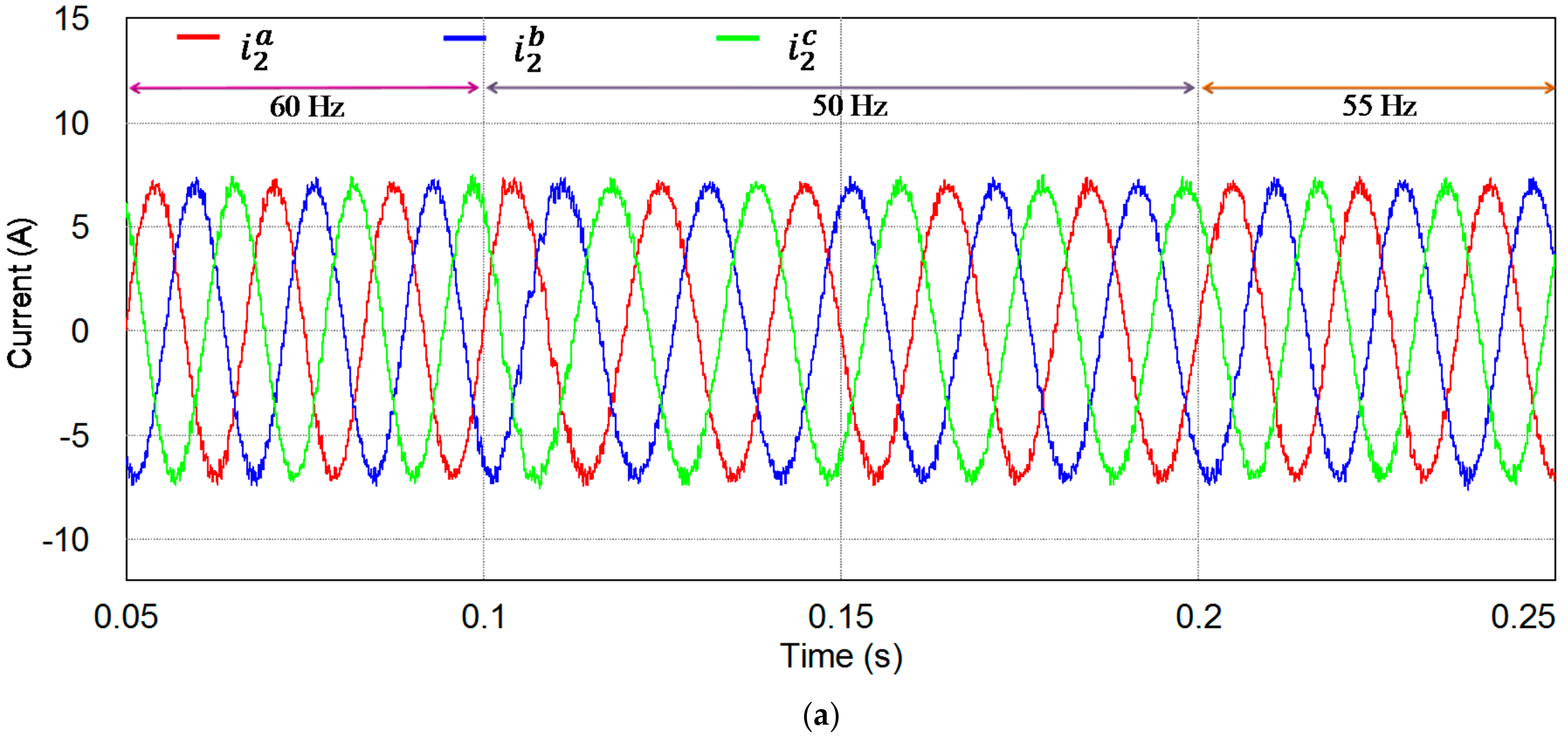
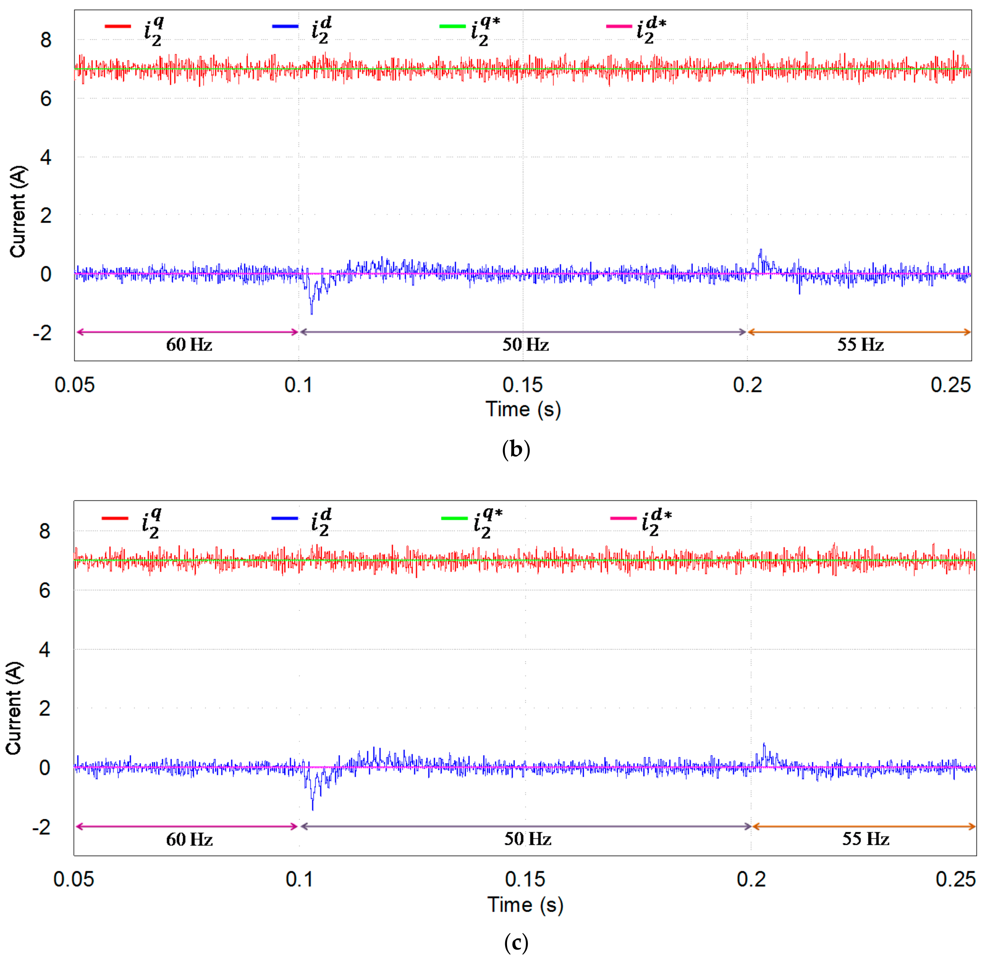
4.2. Control Performance with Frequency Variation

Figure 8 shows the simulation results for the proposed current control scheme under the same grid voltage condition as in Figure 7 when the grid frequency is changed from 60 Hz to 50 Hz at 0.1 s and from 50 Hz to 55 Hz at 0.2 s. These figures represent the responses of the three phase variables for the grid-side currents, inverter-side currents, and capacitor voltages, respectively. Even though the grid voltages are severely distorted and have a step change in frequency, the proposed control scheme provides good harmonic compensation capability, giving quite sinusoidal phase currents without noticeable distortion. The THD values of the grid-side phase currents at steady-state are only 3.76% under 60 Hz, 3.54% under 50 Hz, and 3.45% under 55 Hz in spite of severe distortion of the grid voltages.

Figure 9 shows the simulation results demonstrating the transient response of the grid-side currents of the proposed control scheme, in which Figure 9a shows the instant of frequency change from 60 Hz to 50 Hz at 0.1 s and Figure 9b shows that from 50 Hz to 55 Hz at 0.2 s. It can be clearly confirmed from these figures that the proposed control stabilizes the system rapidly, even under frequency variation, and compensates the current harmonics effectively, maintaining the currents as sinusoidal.

Similar to Figure 9, Figure 10 shows the simulation results demonstrating the transient response of the proposed control scheme. In this figure, the current references and grid-side current responses are presented in the SRF at the instant of frequency change. Except for small current oscillation during the transient periods, the grid-side currents in the q axis and d axis track the references quickly even when the grid frequency varies, which proves the transient performance of the proposed control scheme.

For evaluating the estimation performance of the discrete-time full-state current observer at the stationary reference frame under frequency variation, Figure 11 shows the simulation results under distorted grid and frequency change. Similarly, Figure 11 represents the respective measured and estimated states for the grid-side currents, inverter-side currents, and capacitor voltages in the stationary frame. Evidently, the states estimated by the observer can follow the measured values well even in the presence of frequency variation. This is due to the fact that the observer is designed with the system model in the stationary reference frame, irrespective of frequency information. Furthermore, the gain selection based on the LQR can contribute to obtaining fast and stable operation of the observer.

To evaluate the control performance and robustness of the proposed frequency-adaptive scheme further, the grid impedance variation was considered. Figure 12 shows the simulation results for the reference tracking performance of the proposed control scheme at the SRF. These results were obtained under the condition of distorted grid voltages, frequency changes at 0.1 s and 0.2 s, and the variation of grid inductance $L_2$. In these figures, it is shown that the grid-side currents can track the reference well, even under uncertainty due to the variation of grid inductance, which indicates the fast transient response and robust nature of the proposed control scheme from adopting an LQR control approach.

To verify the quality of injected grid currents for the proposed scheme, Figure 13 shows the FFT result for the steady-state a-phase grid-side current at 60 Hz under harmonic pollution in the grid voltage. This figure also represents the harmonic limits specified by the grid interconnection regulation IEEE Std. 1547 [34]. As can be observed, the harmonic components in the 5th, 7th, 11th, and 13th orders of the injected grid currents can be effectively damped by the proposed control scheme, yielding a THD value of only 3.76%. This meets the quality criteria specified by the grid interconnection regulation IEEE Std. 1547 for inverter-injected current.

In order to validate the effectiveness of the proposed control scheme in different operating conditions, Figure 14 demonstrates the simulation result of the three-phase grid-side currents when the grid voltage is 380 V (line-to-line rms) and the other conditions remain the same as in Figure 8. In spite of the step change in frequency from 60 Hz to 50 Hz at 0.1 s and from 50 Hz to 55 Hz at 0.2 s, the transient response is quite fast. The resultant THD values of the steady-state currents are 3.48% at 60 Hz, 3.34% at 50 Hz, and 3.54% at 55 Hz, which satisfy the standard for harmonic limits specified by the grid interconnection regulation. It is obvious that the proposed control scheme still operates effectively even when the grid voltage is changed.

5. Experimental Results

5.1. Configuration of the Experimental System

Figure 15a shows the experimental system used to implement the proposed current control scheme; the entire system consists of a three-phase grid-connected inverter with an LCL filter, a magnetic contactor for grid connection, a DSP-based controller, and a three-phase programmable AC source to emulate distorted grid voltage and grid frequency variation. For the implementation, only the grid-side current sensors and grid voltage sensors were employed for measurement. The control algorithm was implemented on a 32-bit floating-point DSP TMS320F28335 with a sampling period of 100 µs to control the 2 kVA prototype grid-connected inverter [35]. Figure 15b shows a photograph of the experimental test setup.

Figure 16a presents three-phase distorted grid voltages produced by the programmable AC power source used for performance evaluation in the experiments. As in Figure 4, the grid voltages also have the 5th, 7th, 11th, and 13th harmonics with magnitudes of 5% of the fundamental component. Figure 16b represents the FFT result for the a-phase grid voltage.

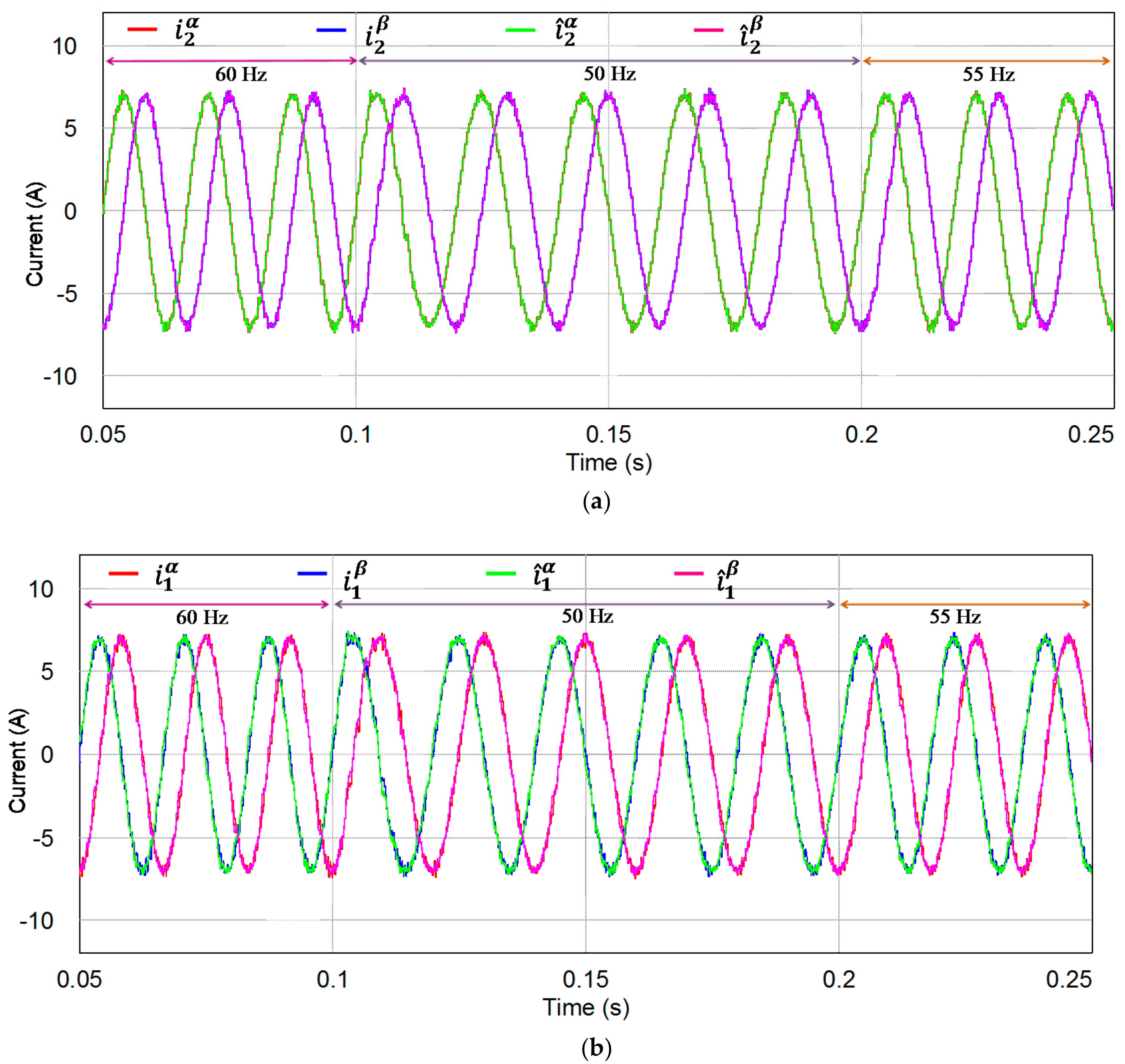
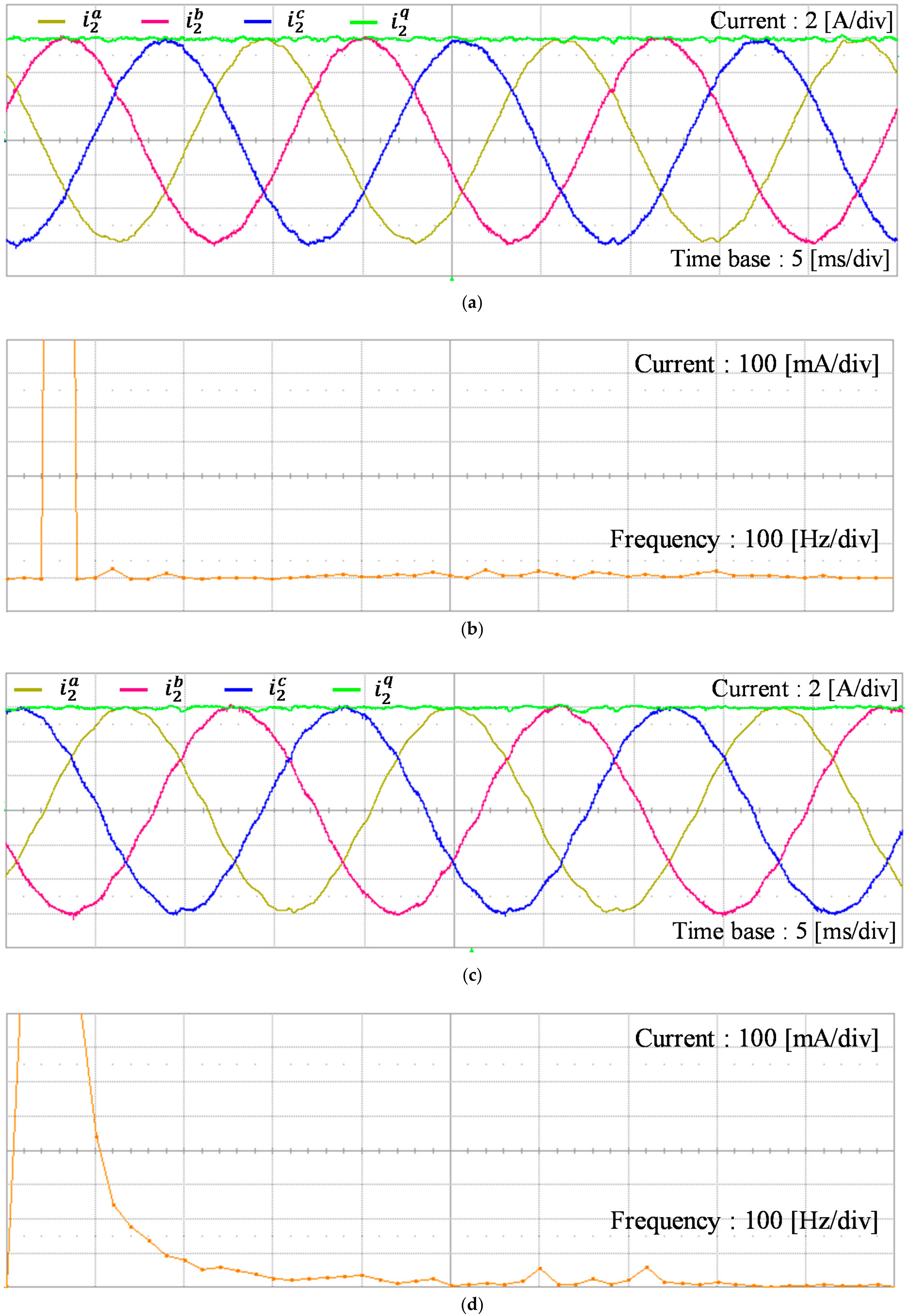
5.2. The Observer’s Estimation Performance

Figure 17 presents the experimental result for the estimation performance of the discrete-time full-state current observer at the stationary frame under step changes in the reference current from 4 A to 6 A. The performance of the proposed control scheme fairly relies on the estimating performance of the observer. Similar to the simulation results in Figure 6, the estimated states well converge to measured states with a fast transient response and stable operation during the transients.

To evaluate the estimating performance of the discrete-time full-state current observer, Figure 18 shows the experimental results for estimated three-phase inverter-side currents and capacitor voltages. In Figure 18a, the estimated three-phase inverter-side currents ${\widehat{i}}_1^a$, ${\widehat{i}}_1^b$, and ${\widehat{i}}_1^c$ were constructed in a DSP by using the estimates ${\widehat{i}}_1^{\alpha }$ and ${\widehat{i}}_1^{\beta }$ at the stationary frame. In a similar way, in Figure 18c, the estimated three-phase capacitor voltages ${\widehat{v}}_c^a$, ${\widehat{v}}_c^b$, and ${\widehat{v}}_c^c$ were calculated from the estimated values ${\widehat{v}}_c^{\alpha }$ and ${\widehat{v}}_c^{\beta }$ at the stationary frame where the observer was designed. The estimated three phase variables are compared with the real measured values in Figure 18b,d. These estimation results clearly confirm the validity and performance of the discrete-time full-state current observer at the stationary reference frame.

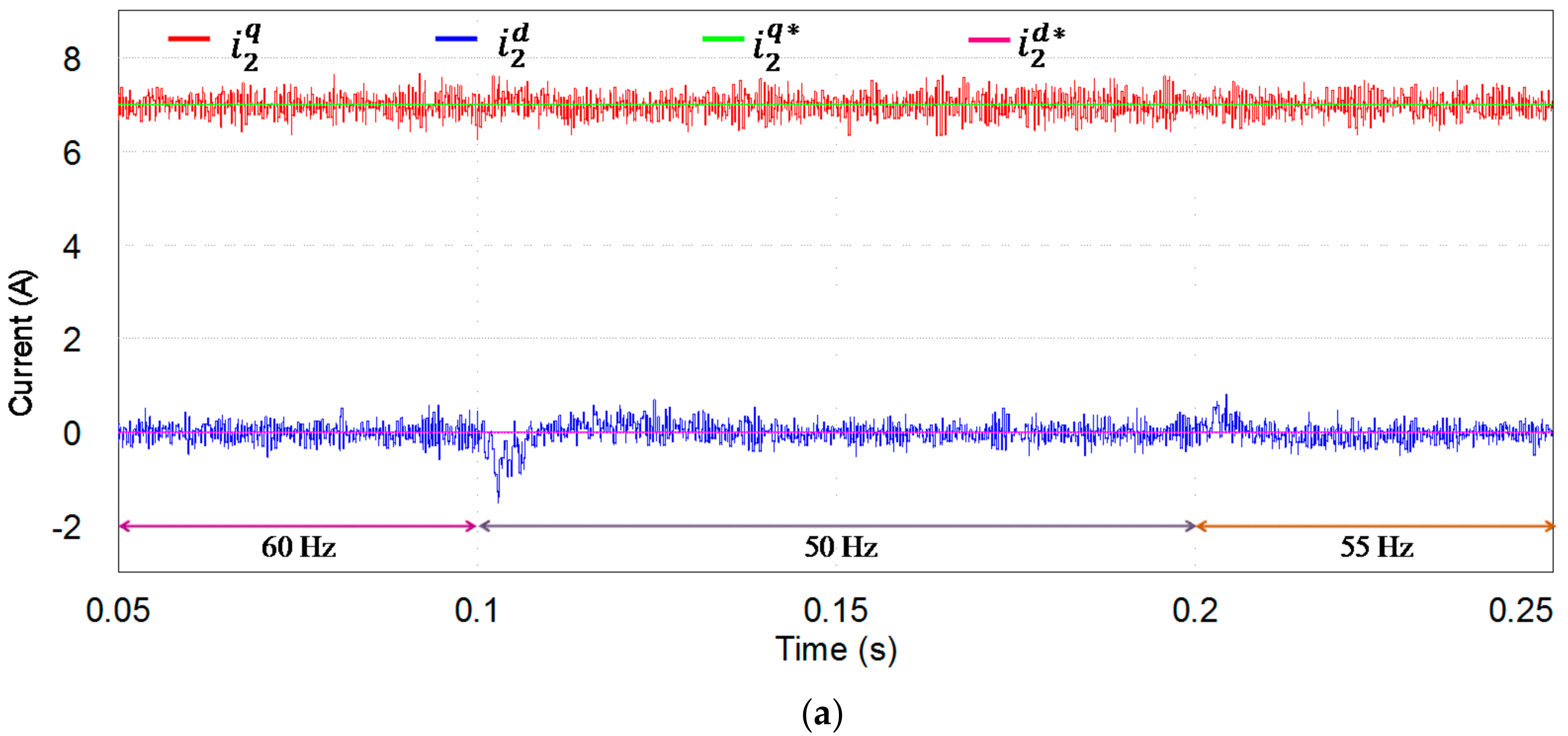
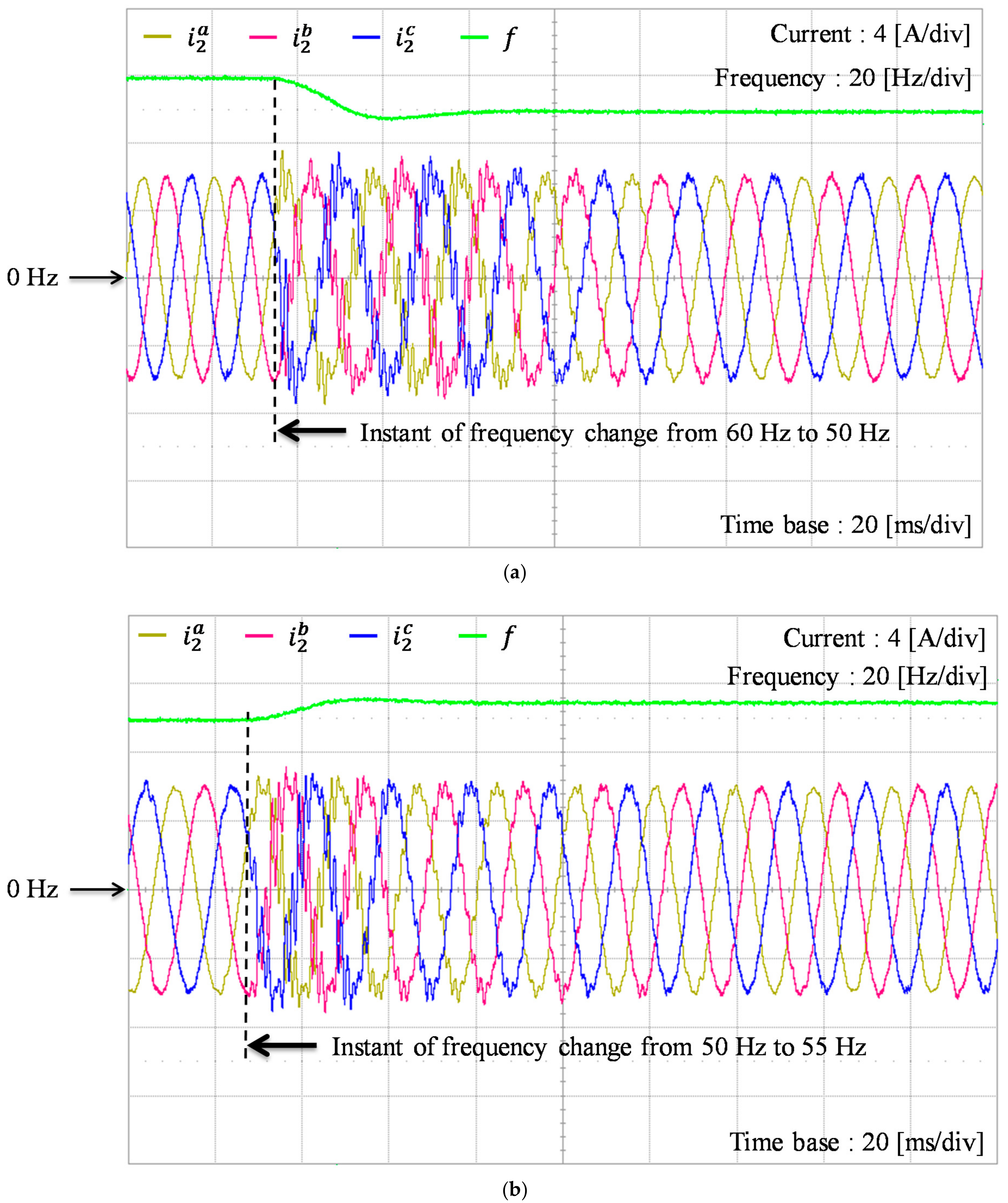
5.3. Control Performance with Frequency Variation

Figure 19 presents the experimental results of the transient response of the proposed frequency-adaptive control scheme under both distorted grid voltages and frequency variation. The frequency estimation and three-phase grid-side current responses are shown in Figure 19a when the grid frequency is instantaneously changed from 60 Hz to 50 Hz. To obtain the frequency information without the fluctuation caused by harmonically distorted grid voltages, the PLL output was processed by the MAF as shown in Figure 3. The obtained fundamental grid frequency $\tilde{\omega }$ is employed in Equation (20) to construct the resonant control for harmonic compensation caused by a distorted grid. Even though the grid-side currents are polluted with harmonics during the transient estimating period of frequency, current waveforms are recovered within five fundamental cycles which are approximately equal to 100 ms, remaining quite sinusoidal afterward. Figure 19b shows the frequency estimation and three-phase grid-side current responses when the grid frequency is instantaneously changed from 50 Hz to 55 Hz. Similarly, it is observed that sinusoidal grid-side currents can be also obtained in five fundamental cycles, which demonstrates the fast transient response of the proposed scheme. On the other hand, in the experimental result of the control method presented in reference [10], it takes approximately 1 s for the controller to compensate the effect of frequency variation when the grid frequency rises from 50 Hz to 53 Hz. In case of the frequency drop from 50 Hz to 47 Hz, the controller needs about 1.4 s to stabilize the system. Obviously, the transient response in that study [10] is longer in comparison with that of the proposed control scheme in both scenarios of frequency increase and decrease in the grid voltage.

To present the steady-state control performance of the proposed scheme, Figure 20 shows the experimental results for the grid-side current waveforms and FFT result of the a-phase current at 60 Hz, 55 Hz, and 50 Hz under a distorted grid condition and frequency variation. In general, the distorted grid voltage directly affects the quality of grid-side currents and degrades the quality of injected power to the grid. However, the proposed scheme yields nearly sinusoidal three-phase currents even under different operating frequencies as shown in Figure 20a,c,e. The FFT results for the a-phase current in Figure 20b,d,f clearly show that the harmonic components in the output current can be effectively damped to negligibly small values. This successfully meets the requirements for the harmonic limits specified by the grid interconnection regulation.

6. Conclusions

In order to overcome the issues relating to both harmonic distortion and frequency variation in grid voltage, a frequency-adaptive current control design for an LCL-filtered grid-connected inverter based on the LQR state feedback control approach was presented. The proposed control scheme is implemented in the SRF by employing the internal model principle for the augmentation of the system model with integral and resonant terms to guarantee the system stability and to achieve asymptotic reference tracking and disturbance rejection. To construct the resonant controller, accurate information on the frequency is essential. In general, however, the frequency extracted from the conventional PLL shows fluctuations under a harmonically distorted grid voltage. In order to avoid performance degradation of the current controller under frequency variation, the frequency extracted from the PLL block is processed by the MAF for the purpose of eliminating the frequency fluctuation due to grid distortion. The filtered frequency information is employed to synthesize the resonant controllers to ensure a high quality of grid currents even in the environment of frequency variation.

Furthermore, in order to reduce the need for additional sensing devices in a grid-connected inverter system equipped with an LCL filter, a discrete-time full-state current observer is employed in the stationary reference frame to estimate all the system states. The advantage of adopting an observer design in the stationary frame and the estimating performance of the observer were discussed in detail. Due to the augmentation of the inverter model with several control terms, an increasing number of feedback gains should be selected. To systematically choose desirable gains for the integral-resonant full-state feedback controller and full-state observer, an LQR approach was introduced. The variation of the grid impedance was also considered as parameter uncertainty to prove the robustness of the proposed control scheme further.

To validate the usefulness of the proposed control scheme, the entire control algorithm was implemented on a 32-bit floating-point DSP TMS320F28335 used to control a 2 kVA prototype grid-connected inverter. The simulation and experimental results were presented for both harmonic distortion and frequency variation in the grid voltage in order to assess the performance of the proposed control scheme. The results show that good reference tracking and harmonic compensation can be accomplished by the proposed scheme even under these conditions by using only the grid-side current sensors and grid voltage sensors. The resultant THD values of the steady-state injected grid-side currents were 3.76 % at 60 Hz, 3.54% at 50 Hz, and 3.45% at 55 Hz, which successfully meet the standard for the harmonic limit. The proposed control scheme was verified under different conditions such as grid distortion, frequency variation, and grid impedance variation. In addition, relatively large frequency variations of 5 Hz and 10 Hz were chosen in order to evaluate the proposed control scheme under more severe conditions. The transient current response under frequency change is very fast, and it takes approximately 100 ms for the controller to stabilize the system.

References

1. Chen, D.; Zhang, J.; Qian, Z. An improved repetitive control scheme for grid-connected inverter with frequency-adaptive capability. IEEE Trans. Ind. Electr. 2013, 60, 814–823. [Google Scholar] [CrossRef]
2. Trinh, Q.N.; Lee, H.H. An advanced current control strategy for three-phase shunt active power filters. IEEE Trans. Ind. Electr. 2013, 60, 5400–5410. [Google Scholar] [CrossRef]
3. Jiang, S.; Cao, D.; Li, Y.; Liu, J.; Peng, F.Z. Low-THD, fast-transient, and cost-effective synchronous-frame repetitive controller for three-phase UPS inverters. IEEE Trans. Power Electr. 2012, 27, 2994–3005. [Google Scholar] [CrossRef]
4. Castilla, M.; Miret, J.; Matas, J.; Garcia de Vicuna, L.; Guerrero, J.M. Linear current control scheme with series resonant harmonic compensator for single-phase grid-connected photovoltaic inverters. IEEE Trans. Ind. Electr. 2008, 55, 2724–2733. [Google Scholar] [CrossRef]
5. Dou, X.; Yang, K.; Quan, X.; Hu, Q.; Wu, Z.; Zhao, B.; Li, P.; Zhang, S.; Jiao, Y. An optimal PR control strategy with load current observer for a three-phase voltage source inverter. Energies 2015, 11, 1–21. [Google Scholar] [CrossRef]
6. Schiesser, M.; Waterlain, S.; Marchesoni, M.; Carpita, M. A simplified design strategy for multi-resonant curent control of a grid-connected voltage source inverter with an LCL filter. Energies 2018, 11, 1–15. [Google Scholar] [CrossRef]
7. Shen, G.; Zhu, X.; Zhang, J.; Xu, D. A new feedback method for PR current control of LCL-filter-based grid-connected inverter. IEEE Trans. Ind. Electr. 2010, 57, 2033–2041. [Google Scholar] [CrossRef]
8. Liserre, M.; Teodorescu, R.; Blaabjerg, F. Multiple harmonics control for three-phase grid converter systems with the use of PI-RES current controller in a rotating frame. IEEE Trans. Power Electr. 2006, 21, 836–841. [Google Scholar] [CrossRef]
9. Li, W.; Ruan, X.; Pan, D.; Wang, X. Full-feedforward schemes of grid voltage for a three-phase LCL-type grid-connected inverter. IEEE Trans. Ind. Electr. 2013, 60, 2237–2249. [Google Scholar] [CrossRef]
10. Huerta, F.; Pérez, J.; Cóbreces, S. Frequency-adaptive multiresonant LQG state-feedback current controller for LCL-filtered VSCs under distorted grid voltages. IEEE Trans. Ind. Electr. 2018, 65, 8433–8444. [Google Scholar] [CrossRef]
11. Yang, Y.; Zhou, K.; Wang, H.; Blaabjerg, F.; Wang, D.; Zhang, B. Frequency adaptive selective harmonic control for grid-connected inverters. IEEE Trans. Ind. Electr. 2015, 30, 3912–3924. [Google Scholar] [CrossRef]
12. Jorge, S.G.; Busada, C.A.; Solsona, J.A. Frequency-adaptive current controller for three-phase grid-connected converters. IEEE Trans. Ind. Electr. 2013, 65, 4169–4177. [Google Scholar] [CrossRef]
13. Eren, S.; Pahlevani, M.; Bakhshai, A.; Jain, P. A digital current control technique for grid-connected AC/DC converters used for energy storage systems. IEEE Trans. Power Electr. 2017, 32, 3970–3988. [Google Scholar] [CrossRef]
14. Hogan, D.J.; Gonzalez-Espin, F.J.; Hayes, J.G.; Lightbody, G.; Foley, R. An adaptive digital-control scheme for improved active power filtering under distorted grid conditions. IEEE Trans. Ind. Electr. 2018, 65, 988–999. [Google Scholar] [CrossRef]
15. Golestan, S.; Ebrahimzadeh, E.; Guerrero, J.M.; Vasquez, J.C. An adaptive resonant regulator for single-phase grid-tied VSCs. IEEE Trans. Power Electr. 2018, 33, 1867–1873. [Google Scholar] [CrossRef]
16. Kukkola, J.; Hinkkanen, M.; Zenger, K. Observer-based state-space current controller for a grid converter equipped with an LCL filter: Analytical method for direct discrete-time design. IEEE Trans. Ind. Appl. 2015, 51, 4079–4090. [Google Scholar] [CrossRef]
17. Yoon, S.J.; Lai, N.B.; Kim, K.H. A systematic controller design for a grid-connected inverter with LCL filter using a discrete-time integral state feedback control and state observer. Energies 2018, 11, 1–20. [Google Scholar]
18. Kukkola, J.; Hinkkanen, M. Observer-based state-space current control for a three-phase grid-connected converter equipped with an LCL filter. IEEE Trans. Ind. Appl. 2014, 50, 2700–2709. [Google Scholar] [CrossRef]
19. Perez-Estevez, D.; Doval-Gandoy, J.; Yepes, A.; Lopez, O. Positive- and negative-sequence current controller with direct discrete-time pole placement for grid-tied converters with LCL filter. IEEE Trans. Power Electr. 2017, 32, 7207–7221. [Google Scholar] [CrossRef]
20. Tran, T.V.; Yoon, S.J.; Kim, K.H. An LQR-based controller design for an LCL-filtered grid-connected inverter in discrete-time state-space under distorted grid environment. Energies 2018, 11, 1–28. [Google Scholar] [CrossRef]
21. Miskovic, V.; Blasko, V.; Jahns, T.M.; Smith, A.H.C.; Romenesko, C. Observer-based active damping of LCL resonance in grid-connected voltage source converters. IEEE Trans. Ind. Appl. 2014, 50, 3977–3985. [Google Scholar] [CrossRef]
22. Francis, B.; Wonham, W. The internal model principle of control theory. Automatica 1976, 12, 457–465. [Google Scholar] [CrossRef]
23. Lai, N.B.; Kim, K.H. Robust control scheme for three-phase grid-connected inverters with LCL-filter under unbalanced and distorted grid conditions. IEEE Trans. Energy Convers. 2018, 33, 506–515. [Google Scholar] [CrossRef]
24. Lim, J.S.; Park, C.; Han, J.; Lee, Y.I. Robust tracking control of a three-phase DC–AC inverter for UPS applications. IEEE Trans. Ind. Electr. 2014, 61, 4142–4151. [Google Scholar] [CrossRef]
25. Maccari, L.A.; Massing, J.R.; Schuch, L.; Rech, C.; Pinheiro, H.; Oliveira, R.C.L.F.; Montagner, V.F. LMI-based control for grid-connected converters with LCL filters under uncertain parameters. IEEE Trans. Power Electr. 2014, 29, 3776–3785. [Google Scholar] [CrossRef]
26. Gabe, I.J.; Montagner, V.F.; Pinheiro, H. Design and implementation of a robust current controller for VSI connected to the grid through an LCL filter. IEEE Trans. Power Electr. 2009, 24, 1444–1452. [Google Scholar] [CrossRef]
27. Franklin, G.; Workman, M.; Powell, J. Digital Control of Dynamic Systems; Ellis-Kagle Press: Half Moon Bay, CA, USA, 2006. [Google Scholar]
28. Golestan, S.; Ramezani, M.; Guerrero, J.M.; Freijedo, F.D.; Monfared, M. Moving average filter based phase-locked loops: Performance analysis and design guidelines. IEEE Trans. Power Electr. 2014, 29, 2750–2763. [Google Scholar] [CrossRef]
29. Orellana, M.; Grino, R. Some consideration about discrete-time AFC controllers. In Proceedings of the 52nd IEEE Conf. on Decision and Control, Florence, Italy, 10–13 December 2013; pp. 6904–6909. [Google Scholar]
30. Dorf, R.C.; Bishop, R.H. Modern Control Systems, 7th ed.; Prentice Hall: Upper Saddle River, NJ, USA, 2008. [Google Scholar]
31. Phillips, C.L.; Nagle, H.T. Digital Control System Analysis and Design, 3rd ed.; Prentice Hall: Englewood Cliffs, NJ, USA, 1995. [Google Scholar]
32. Ogata, K. Discrete Time Control Systems, 2nd ed.; Prentice Hall: Englewood Cliffs, NJ, USA, 1995. [Google Scholar]
33. Huerta, F.; Pizarro, D.; Cóbreces, S.; Rodríguez, F.J.; Girón, C.; Rodríguez, A. LQG servo controller for the current control of LCL grid-connected voltage-source converters. IEEE Trans. Ind. Electr. 2012, 59, 4272–4284. [Google Scholar] [CrossRef]
34. IEEE. IEEE Standard for Interconnecting Distributed Resources with Electric Power System; IEEE Std.1547; IEEE: New York, NY, USA, 2003. [Google Scholar]
35. Texas Instrument. TMS320F28335 Digital Signal. Controller (DSC)—Data Manual; Texas Instrument: Dallas, TX, USA, 2008. [Google Scholar]
Figure 1. Configuration of a grid-connected inverter with an inductive–capacitive–inductive (LCL) filter.
Energies 11 02674 g001
Figure 2. Block diagram of the proposed frequency-adaptive current control scheme.
Energies 11 02674 g002
Figure 3. Block diagram of frequency detection based on the MAF under distorted grid voltage.
Energies 11 02674 g003
Figure 4. Three-phase grid voltages with harmonic distortion. (a) Distorted grid voltages; (b) FFT result of a-phase grid voltage.
Energies 11 02674 g004
Figure 5. Simulation result for the current control performance with an integral-resonant state feedback control under distorted grid voltage. Current references and grid-side current responses at the synchronous reference frame (SRF).
Energies 11 02674 g005
Figure 6. Simulation results for the discrete-time full-state current observer at the stationary reference frame under step changes in the reference current. Measured and estimated waveforms. (a) Grid-side currents and estimated states; (b) Inverter-side currents and estimated states; (c) Capacitor voltages and estimated states.
Energies 11 02674 g006
Figure 7. Three-phase distorted grid voltages with frequency changes at 0.1 s and 0.2 s.
Energies 11 02674 g007
Figure 8. Simulation results for the proposed control scheme with frequency changes at 0.1 s and 0.2 s. Three-phase measured waveforms. (a) Three-phase grid-side currents; (b) Three-phase inverter-side currents; (c) Three-phase capacitor voltages.
Energies 11 02674 g008aEnergies 11 02674 g008b
Figure 9. Simulation results for the transient response with frequency change. (a) Three-phase grid-side currents with frequency change from 60 Hz to 50 Hz at time 0.1 s; (b) Three-phase grid-side currents with frequency change from 50 Hz to 55 Hz at time 0.2 s.
Energies 11 02674 g009
Figure 10. Simulation result for the transient response of the proposed control scheme with frequency changes at 0.1 s and 0.2 s. Current references and grid-side current responses at the SRF.
Energies 11 02674 g010
Figure 11. Simulation results for the discrete-time full-state current observer at the stationary reference frame with frequency changes at 0.1 s and 0.2 s. Measured and estimated waveforms at the stationary reference frame. (a) Grid-side currents and estimated states; (b) Inverter-side currents and estimated states; (c) Capacitor voltages and estimated states.
Energies 11 02674 g011aEnergies 11 02674 g011b
Figure 12. Simulation results for the reference tracking performance of the proposed control scheme with frequency changes at 0.1 s and 0.2 s under the variation of grid inductance L 2 . Current references and grid-side current responses at the SRF (a) with L 2 = 1.3   mH ; (b) with L 2 = 2.1   mH ; and (c) with L 2 = 2.5   mH .
Energies 11 02674 g012aEnergies 11 02674 g012b
Figure 13. FFT result for the a-phase grid-side current of the proposed control scheme under distorted grid conditions.
Energies 11 02674 g013
Figure 14. Simulation result for the proposed control scheme with frequency changes at 0.1 s and 0.2 s when the grid voltage is 380 V (line-to-line rms). Three-phase grid-side currents.
Energies 11 02674 g014
Figure 15. Experimental system. (a) Configuration of the overall system; (b) Photograph of the experimental test setup.
Energies 11 02674 g015
Figure 16. Three-phase distorted grid voltages produced by the programmable AC source in experiments. (a) Three-phase distorted voltages; (b) FFT result of the a-phase grid voltage.
Energies 11 02674 g016
Figure 17. Experimental result for the discrete-time full-state current observer under step changes in the reference current. Measured and estimated grid-side currents at the stationary frame.
Energies 11 02674 g017
Figure 18. Experimental results of the estimating performance of the discrete-time full-state current observer at the stationary frame under step changes in the reference current. (a) Estimated three-phase inverter-side currents; (b) Comparison of the estimated and measured inverter-side currents; (c) Estimated three-phase capacitor voltages; (d) Comparison of the estimated and measured capacitor voltages.
Energies 11 02674 g018aEnergies 11 02674 g018b
Figure 19. Experimental results for the transient response of the proposed frequency-adaptive control scheme in the presence of both distorted grid voltages and frequency change. (a) Frequency estimation and three-phase grid-side current response under frequency change from 60 Hz to 50 Hz; (b) Frequency estimation and three-phase grid-side current response under frequency change from 50 Hz to 55 Hz.
Energies 11 02674 g019
Figure 20. Experimental results for the steady-state grid-side currents of the proposed frequency-adaptive control scheme under both distorted grid voltages and frequency change. (a) Grid-side currents at 60 Hz; (b) FFT result for the a-phase current at 60 Hz; (c) Grid-side currents at 55 Hz; (d) FFT result for the a-phase current at 55 Hz; (e) Grid-side currents at 50 Hz; (f) FFT result for the a-phase current at 50 Hz.
Energies 11 02674 g020aEnergies 11 02674 g020b