1. Introduction
Crude oil, as well as its derivatives, such as gasoline and heating oil, are among the most commonly traded commodities for decades. Crude oil price is still serving as a benchmark for the pricing of other commodities, such as natural gas. The initial penetration of natural gas was based on the formation of long-term crude oil linked contracts, aiming at becoming a substitute of crude oil for industrial and heating purposes. However, the increasing volumes in natural gas trading has created dynamics for fully integrated natural gas markets, triggering the research on unveiling the time-varying linkages between crude oil and natural gas prices.
The relationship between crude oil and natural gas prices has been strongly challenged in the US, as the fundamentals of crude oil and natural gas market changed considerably, due to the evolution of shale oil and shale gas. The rise of the unconventional oil production created oversupply conditions, which -together with the strategy of the Organization of the Petroleum Exporting Countries (OPEC) to not decrease its production- have caused a sharp decrease in crude oil prices, i.e., West Texas Intermediate fell at the
$26 per barrel in 2016. This has led the US unconventional oil producing companies to initiate programmes of cost reduction, efficiency improvement, or even the mothball of wells. On the other hand, shale gas producers continued their production almost uninterrupted, as the US Lower 48 Production declined only by just over one billion cubic feet per day. This was justified by the fact that the demand for natural gas had different pattern compared to that of oil, as the power generation by natural gas units overtook that of coal [
1].
According to the BP energy outlook [
2] the gas market and system is rapidly evolving in the US and globally. The US global oil production share rises to 18% from 12% by 2040, which is even higher than that of Saudi Arabia, the second largest producer with a market share of 13% in 2040. Shale gas production constitutes US an even greater hydrocarbon producer as its global production share will be 24% in 2040, and will leave the Russian Federation second with 14%. The aforementioned developments should be considered with the projection that the US will be the largest consumer of gas and the second largest consumer of oil. This will leave the market tighter with few exporting margins. The projected exports will be 360 Million Tonnes of oil equivalent (Mtoe) for oil and gas combinedly, which will be around the 9% of global trade in oil and gas in 2016. The Russian Federation will remain the largest exporter with a total of 780 M toe of oil and gas in 2040.
Contrary to other regions, the US domestic gas market is already large and mature, where about half of the US households are gas heated. According to the Energy Information Administration (EIA) winter fuels outlook [
3] projections for increased demand are expected to lead to a price increase, as US households are expected to need
$69 more to be heated, or there will be a 12% increase compared to the previous winter, with 9% driven by consumption and 2% by price. The average price for residential consumption is estimated at
$10.36 per thousand cubic feet (Mcf). Strong demand will drive Henry Hub spot prices to an average of
$3.18 per Million British Thermal Units (MMBTU) or
$3.30/Mcf, 5% higher than previous winter. The situation in the US is transitory, as pipeline bottlenecks continue to exist in the Appalachian region making it difficult to carry quantities from the gas rich regions of Marcellus and Utica in Ohio, Pennsylvania and West Virginia. The projected gas inventories were approximately estimated at 3.8 trillion cubic feet by the end of October 2017.
The latest updates pose a question on the price interdependencies between crude oil and natural gas in the US markets. The US is an interesting case study, as the US are rapidly transforming from an oil and gas importer to an exporter, due to the unconventional production. It is also an interesting example for other regions as, apart from the supply shock, the domestic market made great steps towards integration with the interstate gas pipeline deregulation, based on the legislation issued by the Federal Energy Regulatory Commission (FERC) in 2000 [
4]. However, the gas exporting facilities and the infrastructure remain largely not fully developed or utilised, which delays the increased liquidity of regional natural gas hubs and the evolution for a global integrated natural gas market. The Oxford Institute for Energy Studies discerns gas hub markets, in order to evaluate them for their liquidity and transparency, by five key elements. These are the number of participants, the traded products, the traded volumes, the tradability index, and the churn rates [
5]. Henry Hub can claim that champions in all these key elements, and as a matter of fact be perceived as a role model for other regions. E.U. for example has adopted the European Gas Target model strategy, which aims at enhancing its security of supply, the development of a fully functioning natural gas wholesale market and a flexible role for gas in electricity generation complementing the renewable production [
6]. The above analysis identifies that the US natural gas market has been evolved as the most integrated and mature regional gas market. Since the market is integrated, it is interesting to study whether gas or oil are priced independently from other commodities or the rule of one commodity pricing still holds, and apply its conclusion to different regional markets.
There is an extended literature review on the linkages between natural gas and crude oil markets or other oil derivatives, both at regional or global level. The oil and gas price and volatility spillovers are dynamically evolved through time. In our analysis, we aim to capture their time varying relationship, by examining data up to the latest complete year 2017., by examining data up to year 2017.
Villar and Joutz [
7] suggest that there is a cointegrating relationship between natural gas and crude oil. The prices between Henry Hub and WTI have a long run relationship. Erdos [
8] finds that between 1997 and 2008 the US oil and gas prices co-moved in the short run and were cointegrated in the long run. Since 2009, the US natural gas prices and the European gas and crude prices have decoupled. He further supports that between 1997 and 2008, there were imports from Europe to US, as US gas prices were higher. This course is reversed since 2009, as there is an oversupply in the US and a lack of extended supply diversification in Europe. Due to the lack and low utilization of exporting facilities, and the regional gas oversupply, the US gas prices gradually decoupled from oil prices and from European or Asian oil-indexed gas markets. Asche et al. [
9] find that oil and gas prices can present high differences in short term, but these are eliminated in the long run. The long term equilibrium is justified by the substitution between oil and gas.
Lin and Li [
10] suggest that the European and Japanese gas prices have a long term relationship, i.e., cointegration with Brent crude oil prices. On the contrary, this does not apply for the US market. This is due to the existence of oil-indexed contracts in Europe and Japan, while the US gas market depends more on its own market fundamentals for price formulation. They also add that even if US oil and gas prices are decoupled, then oil prices changes could still be spilled over the gas prices. Jadidzadeh and Serletis [
11] propose that natural gas’ price response differs greatly, due to the nature of the oil price shock. They add that 45% of the natural gas price variation is attributed to the aggregate demand and supply shocks. They conclude that natural gas price is decoupled from oil price. Nick and Thoenes [
12] suggest that abnormal temperatures and supply shocks account only for the short term fluctuation of the natural gas price, when crude oil and coal prices account for the price development in the long run. They also add that supply shocks have a significant impact on the German gas market, although they were exacerbated by simultaneous extraordinary demand.
Malik and Ewing [
13] find that oil price volatility has a number of interdependencies with other market sectors, concluding that this kind of relationship can be used as a hedging mean. They point out that since many financial instruments are index-based, this kind of volatility transmission might be useful for optimal portfolio allocation. Wakamatsu and Agura [
14] detect 2005 as the break point of the relationship between the Japanese and US gas market, which is attributed to the shale gas revolution occurred in the US. US market followed a more independent course since 2005. This might alter if considerable US gas exports are allowed and gas starts to penetrate the Japanese gas market. Their study also presents the inelastic relationship of gas consumption to income, as gas is perceived as a necessary good. Geng et al. [
15] suggest that the seasonal effect on gas price evolution, which was present in the US gas market before the shale revolution and disappeared, due to the sudden gas oversupply. Moreover, WTI price and Henry Hub prices were cointegrated before the shale gas production increase, however they are now decoupled. On the contrary, European gas markets have not been influenced by the shale gas oversupply, and they largely remain dependent on crude oil price patterns. This kind of conditions might change if European countries diversify their supply sources and pricing formulas. Geng et al. [
16] suggest that WTI and Brent prices had a significant impact on Henry Hub and National Balancing Point (NBP) prices respectively, but this changed as US shale revolution made WTI to have weak influence, while European gas market remained exposed to oil price volatility. They proceed by proposing that the oil impact on natural gas prices has disappeared for medium and long term horizons. They add that before the shale gas revolution, WTI shocks were more influential to Henry Hub high frequency price fluctuations. On the contrary, low frequency Henry Hub price fluctuations are more vulnerable after the shale gas revolution. Indirect volatility spillovers between gas and oil are present and they are bidirectional. They also find that there is direct volatility linkage from natural gas to oil returns. Batten et al. [
17] present evidence that, since 2007, oil and gas markets are independent and as a consequence they can no longer be perceived as substitutes for hedging reasons. Prior to 2007, there is a unilateral causality from natural gas to oil. They suggest that this independence might be attributed to the shale revolution with the new hydraulic fracturing and horizontal drilling.
Brown and Yucel [
18] study another perspective of the US gas market, as this was early deregulated and endowed with an extended free flowing pipeline system leaving opportunities for regional arbitrage. However, transmission system operators were not offered incentives for system upgrades and expansions, and as a consequence they did not follow gas consumption. Nevertheless, this led to supply bottlenecks, and regional, operational and technical factors were most important than Henry Hub prices or arbitrage. Brown and Yucel [
19] proceed with suggesting that the US gas prices are determined by gas storages. They also propose that increased regional storages can substitute transmission capacity. If there are no augmented storages, then regional demand can cause sharp price movements.
Honarvar [
20] studies the asymmetries that arise between oil and its derivatives. A positive shock from the crude oil market, keeping retail gasoline price constant, is only transitory. Furthermore, there is a long run asymmetry, which can be attributed to consumers’ responses to technological changes. Ji et al. [
21] propose that crude oil prices have a larger impact on gas prices than global economic activity. The volatility of crude oil prices has different negative impact on natural gas import prices, depending on which regional market is studied. US experience weak influence by crude oil’s volatility shocks. In addition, Europe experiences crude oil’s volatility shocks with a lag for shorter periods and at a weak extent. They also find asymmetric responses, where crude oil price decreases have stronger influence. Atil et al. [
22] support that both natural gas and gasoline adjust to oil price changes. They find that natural gas adjusts to oil price changes slower than gasoline, and they attribute this to gas’ regional character. They also add that negative oil shocks have larger impact than positive ones. Pal and Mitra [
23] use a multiple threshold nonlinear autoregressive distributed lag model to study potential asymmetries between oil and its derivatives. They find that there are differences, whether of direction or magnitude, to the oil derivatives’ price, due to crude oil price changes. They also add that sharp crude oil decreases do not fully pass to oil derivatives’ prices. Wiggins and Etiene [
24] support that natural gas price responds differently to supply and demand shocks. They further conclude that precautionary inventory shocks have lower impact than supply and aggregate demand shocks. Another conclusion of their research is that demand elasticity became more elastic, as consumers can substitute their energy source easier. They also suggest that aggregate demand and supply shocks account for 20% of the post-regulation price volatility. Lin and Wesseh [
25] suggest that regime switching exists in the natural gas market and its volatility is not predictable, as it is not persistent.
The US wholesale markets are of great interest as the evolution of unconventional oil and gas production has challenged their relationship. This evolving relationship has already been examined by several papers, as presented above, leading to some common conclusions, especially related to the price spillovers: The relationship is dynamic and time-varying, price spillovers are mainly from oil to gas, while asymmetric relationship is also evident among price increases and decreases. However, the research on volatility spillovers concerns mainly the relationship between oil with other equity sectors returns, rather than with the natural gas market.
The paper examines both the time-varying price and volatility transmission between US natural gas and crude oil wholesale markets, over the period 1990–2017, using different econometric techniques. The paper contributes by presenting evidence of market decoupling when others consider them as cointegrated (Villar and Joutz [
7] and Brown and Yucel [
19]). Contrary to what is believed like Geng et al. [
16], we add that the shale revolution does not destabilise the long run relationship between the two markets, as they are already decoupled, and only if certain conditions prevail, then there is only influence from oil to gas (threshold cointegration). Further, we study the causal relationship without exogeneity presumptions of any kind, like Nick and Thoenes [
12] do. Our study not only sheds light to the relationship between the two commodities, and challenges presumptions of already work for preceding periods, but also covers the very recent data up to 2017. The examined period incorporates a decade, since the start of the shale revolution, which has transformed the US energy market.
Our paper examines the price and volatility spillovers from natural gas to crude oil and vice versa in the US wholesale markets. We provide updated empirical evidence on the price and volatility transmission, focusing on the time-varying characteristics of US natural gas and crude oil markets. We examine the time-varying relationship with in-sample and out-of-sample methodologies, the asymmetric price transmission, the long-term price impacts and the time-varying volatility transmission among the commodities. We apply several econometric methodologies to derive conclusions: Bivariate Vector Autoregression (VAR) models assuming that oil and gas price variables are endogenous allowing feedback between prices, the Momentum Threshold Autoregressive (MTAR) cointegration for examining asymmetric relationships between prices, out of sample Granger causality tests with Diebold and Mariano forecasting accuracy test, accumulated impulse response functions (AIRF) to examine long-term price relationships, and the Dynamic Conditional Covariance (DCC) Generalized Autoregressive Conditional Heteroscedasticity (GARCH) model to elaborate volatility transmission. Batten et. al. [
17] recently applied the bivariate Vector Autoregressive (VAR) methodology, examining the linkages between crude oil and natural gas, while Ferraro et al. [
26] recently applied the same intuition to examine the linkage between crude oil and exchange rates. The former paper provides also several causality tests, which are also implemented in this paper, using more recent data as well a considerably longer period. The implementation of MTAR and DCC-GARCH methodologies examine asymmetric causality and volatility transmission among the two commodities respectively. The DCC-GARCH methodology is a methodology used in different sectors, such as the papers by Chevallier [
27], Wei [
28] and Singhal and Ghosh [
29].
Our paper is organised as follows: Following the introduction,
Section 2 provides the description of data elaborated.
Section 3 presents the methodologies that have been applied, followed by
Section 4 which provides the empirical results and discussion. Finally,
Section 5 provides the concluding remarks.
2. Data
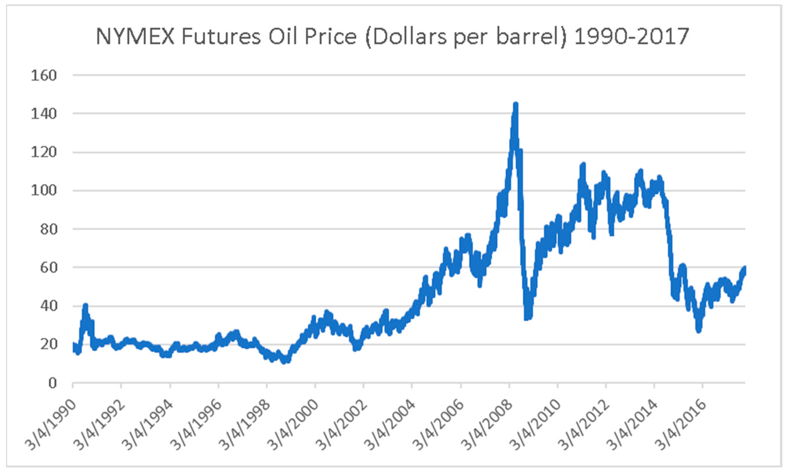
The data used for our analysis are the daily closing prices of the New York Mercantile Exchange (NYMEX) Crude Oil Futures and of the NYMEX Henry Hub. Prices are in US dollars per barrel and Million British Thermal Units (MMBTU) respectively. The data cover the period between 3/4/1990 and 31/12/2017, consisting of 6975 observations and are presented in
Figure 1 and
Figure 2 respectively. Our effort is to include data for full years, and as a matter of fact our data start from the first time NYMEX started offering standardized natural gas contracts with physical delivery at the Henry Hub up to 2017. We have chosen to use the prices of futures as futures’ markets tend to be more liquid and to include adjustments faster than the spot market. For the rest of the paper, NYMEX Crude Oil futures prices and NYMEX Henry Hub prices will be referred as oil and gas prices respectively for reasons of convenience.
As explained above, the study is focused on the US wholesale natural gas and crude oil markets. Nowadays, the two commodity markets are considered to be driven by market dynamics, as oil-indexed gas contracts have been rapidly eliminated to almost 0% for both domestic production and imported gas in North America, as shown in a recent global review of price formation mechanisms by the International Gas Union [
30]. Moreover, a deregulation phase of interstate pipeline system has already taken effect in the domestic US gas market, while the evolution of shale gas proved to be a game changer for regional gas market. Another interesting factor that should be also considered is the US energy policy on the domestic US oil and gas production, which were not exported to the global market, due to the lack of regulatory framework or exporting facilities. While the rest of oil and gas producers, such as Russia, Norway, Qatar or Algeria try to enhance their exporting potentials by expanding pipelines and LNG systems with long term contracts, US followed a different path. Moreover, the majority of contracts of the main producers other than US were based on oil indexed aspects. Studying the US market provides the advantage of examining a more advanced, competitive and integrated natural gas market. In addition, this extended period of more than 28 years covers main events in both commodity markets. Wars in oil producing countries, such as the Gulf War in 1991 [
31], OPEC production decisions, technological advances, such as hydraulic fracking and horizontal drilling [
32], gas deregulation [
4], the financial crisis of 2008, the Deepwater Horizon explosion and oil spill in the Gulf of Mexico, physical phenomena, such as Hurricane Katrina in 2005 [
33] and Fukushima disaster in 2011 [
34], which might have played a major role in price formulation in the largest Mercantile Exchange. All those events are important, however the identification of the statistical importance of any event on a time series is done through the identification of structural breaks. Applying the Bai-Perron multiple structural breakpoint methodology [
35] on the updated dataset, has led to the identification of the structural break on date 10/9/1998 for the gas time series. In case of oil time series, multiple breakpoints were estimated, which indicated that we should follow a refinement procedure from the sequential to the repartition dates, leading to identify the following time periods 03/04/1990–27/11/2001, 28/11/2001–31/03/2009 and 01/04/2009–29/12/2017. Unfortunately, we could not find significant events that could justify the structural breakpoints. When we included the dummy variables derived by the structural breakpoints, we did not have any cointegrating relationship. Their coefficients were also not statistically significant, when we included these dummy variables in our VAR models
Since we examine a regionally integrated gas market and a globally integrated crude oil market, it is easily understood that oil prices are determined by more global economic fundamentals while gas prices may be affected by more regional factors, such as infrastructure sufficiency, i.e., infrastructure bottlenecks like lack of distribution systems or low capacity pipelines might affect the supply side [
18,
19] or lack of exporting facilities might cause local glut and affect regional prices [
36]. Production oversupply and increased gas stocks may moderate this condition. Our study, which is described in the next sections, leads to results that mostly surpass this implication.
3. Methodology
We examine the time-varying relationship with in-sample and out-of-sample methodologies, the asymmetric price transmission, the long-term price impacts and the time-varying volatility transmission among the commodities. Structural breaks are important for some methodologies, such as regression analysis, as their identification clarifies the need for examination of coefficients/elasticities on different time periods. Since the effect of transitory events last for short periods, their effect is restrained in very short iterations and as a matter of fact whenever we tried their influence with dummies we failed to have statistically important coefficients. We included dummies for the structural breaks, as well as the above-mentioned events. However, as mentioned in the previous section, when we included the dummy variables, we did not have any cointegrating relationship while their coefficients were also not statistically significant.
3.1. Time Domain Causality Tests
In this section, our main aim is to investigate whether the price information of one commodity is passed to the other, by examining this relationship over an extended period. Granger [
37] causality tests or Wald tests are our main instrument to examine price spillovers between oil and gas prices and vice versa. Granger causality test investigates whether information included in one variable is able to explain other’s variable course. Granger causality test inherits an assumption that there is a symmetrical relationship between the two variables, i.e., an increase in one variable will have the same magnitude and speed effect as a decrease.
Granger causality tests are calculated as in-sample F or alternatively as Wald test in VAR (Vector Autoregressive) models. In order to proceed with our Wald tests we construct our two models, which will be later characterized as unrestricted, explaining price changes.
ΔOil and ΔGas are the first differences of our data, which are in natural logarithms at time t, where ΔOil
t−p and ΔGas
t−p are the lagged differences of the p class VARs, whose class is determined by the Akaike criterion. Since our variables are in natural logarithms, their first differences are assumed to be the respective returns, if we neglect other cost differentials, such as carrying costs. VAR models assume that our variables are endogenous thus leaving our structural assumption free in regard to the relation between oil and gas, while Kilian [
38] use structured VAR (SVAR) models to examine crude oil price shocks. The method of VAR is that of least squares or OLS. The Granger hypothesis which can be tested for our models is:
while the alternative hypothesis, is:
If the null hypothesis is rejected, then we have causality or price spillovers from one commodity market to the other. In such case, using first commodity’s price is useful in forecasting second’s price.
Since we intend to study the time-varying price relationship between the two commodities, we do not conduct Wald tests only for the full sample period, but we divide it in shorter periods. We use periods of 250 observations, which account for a full year as both commodity markets have approximately 252 working days per year. Our rolling periods proceed every 100th observation using a sample window of 250 observations. By this we account for changes within the years. This kind of iterations are, in our opinion, the most sensitive method to capture the price spillovers, in case they are existent.
3.2. Asymmetric Price Transmission
An inherent assumption of Wald test is that there is a symmetrical relationship between the two variables, i.e., the price increase of the first commodity will have an effect of the same speed and magnitude with a price decrease to the second commodity’s price. In most of the times, this is not the case, and price transmission has different magnitude or speed. Price transmission can have both a vertical and horizontal character. Vertical asymmetric price transmission is between variables of the same marketing chain or sector, where horizontal or spatial price transmission is between different sectors or marketing chains. We consider oil and natural gas markets as two separate individual markets, which operate in different marketing chains. We do not consider that the one market vertically precedes the other in the marketing process. The third discretion of asymmetrical price transmission is on whether this is positive or negative, i.e., if the price of the second variable reacts at a larger extent or faster to an increase of the first variable compared to the same decrease, then the asymmetry is characterized as “positive”. When the opposite holds i.e., the price of the second variable reacts more or faster to a first variable’s decrease, then we have “negative” price asymmetry.
If we consider the price of the first commodity as
and that of the second as
, then we proceed with our study of asymmetric price transmission. We use an Error Correction Model, or ECM, methodology proposed by Engle and Granger [
39] for our asymmetric price transmission research. Granger and Newbold [
40] suggest that regressions between non stationary variables or variables with similar behavior produce spurious results i.e., suggest relationships that do not in reality exist. In order to test whether our variables are stationary or not, we use the Augmented Dickey Fuller test and the Phillips and Perron test (
Table 1). Both tests suggest that our variables are non-stationary. Then we proceed with their first difference, which should be stationary, i.e., they are I(1) and not I(0). Engle and Granger [
39] point out that if I(1) variables are stationary and cointegrated, then the linear relation between them is stationary. In our study we consider the relationship:
If the tests support that Equation (5) is not spurious then and are cointegrated and Equation (5) stands as the long term relationship.
The second step of an Error Correction Model (ECM) is taking the residuals of Equation (5) and use them as the lagged −1 Error Correction Term (ECT).
The ECT presents the deviations from the long run relationship between
and
. Dividing ECT into positive and negative components, i.e., positive and negative corrections from the long run relationship helps to account for asymmetric price transmission. We use the ECM model by Engle and Granger [
39] to reach our second equation.
where Δ
and Δ
are the first differences and
the residuals.
As discussed above, cointegration and ECM analysis are based on the foundation that a long run equilibrium between
and
exists. This kind of relationship prevents the two variables from following independent courses. As a result, Equations (5) and (6) only account for speed asymmetry. Two variables can be cointegrated even if standard tests, such as Johansen test may not verify this long run relationship. This kind of long-term relationship may take only place when one variable’s change exceeds a certain level and up. If a threshold exists for this long run relationship, then we account for threshold cointegration. Tong [
41] introduced the approach of threshold cointegration, where price adjustments only take place if a certain threshold level is exceeded. If ECT lies between the threshold levels, no error correction procedure is present. This band, between the thresholds, represents the area where the adjustment costs are disproportionate to deviation. Goodwin and Piggot [
42] characterize the threshold interval as “neutral band”.
Enders and Granger [
43] introduce Momentum Threshold Autoregressive (MTAR) cointegration, as an asymmetric relationship between two prices cannot be examined by symmetric long-term tests.
In our study we use the MTAR threshold cointegration approach. To our knowledge, this is an innovative approach for this branch of the literature. By this approach, we try to capture the potential threshold where no error correction takes place. This is an additional point, which could not be explored by an asymmetric causality test. We exclude a percentage of our observations in order to determine our threshold value by fitting our regression, and then we use the threshold value with the lowest Sum of Squared Errors (SSE). Since we have the best threshold value, we proceed with lag selection using the Akaike criterion. If threshold cointegration exists, then we proceed with fitting our asymmetric ECM using the best threshold value. All of the procedures for determining the threshold value, lag selection, fitting threshold cointegration and asymmetric ECM are conducted with the MTAR methodology. We use this kind of methodology for both oil and gas as and respectively and vice versa.
3.3. Out of Sample Causality Tests
Since we study price spillovers from one commodity to the other, i.e., information contained in first commodity’s price can be used to forecast second’s commodity price, we can move from in sample Granger causality tests to out of sample ones. In order to proceed with our out of sample tests, we have to estimate the restricted versions of (1) and (2) and then compare their forecasting ability to that of their initial models.
The restricted model for Equation (1) is
for Equation (2) is
Initially, we proceed with the one step ahead forecasts from both the restricted and unrestricted models and then we compare their forecasting accuracy with Diebold and Mariano [
44] test. Diebold and Mariano test assumes that both restricted and unrestricted models will produce forecasts of equal Mean Squared Forecast Errors (MSFE), i.e., they have equal predictive accuracy. If the null hypothesis is rejected, then a model produces forecasts of lower MSFE i.e., has better predictive ability.
In our study we investigate the dynamic relationship between oil and gas, by proceeding with an out of sample one step ahead forecast using the full sample period, and then we proceed by examining shorter periods. In this step we estimate again one step ahead forecasts year by year, and we reveal the time-varying relationship.
3.4 Long Term Impacts
Our research would not be sufficient enough if we did not calculate the cumulative impact that one commodity price change has on the other. The rolling VAR models and their respective Wald tests only calculate the symmetrical probability of the relationship between the variables. Since both commodity markets are considered as highly liquid, we can use a ten-day horizon for our calculations, as this represents two trading weeks. This is due to the fact that gas and oil futures absorb the information fast and fully enough, in very short periods, as there are arbitrage opportunities. The method used is by deriving impulse response functions from the same bivariate rolling VARs.
In order to calculate the full impact, we use Accumulated Impulse Response Functions (AIRF). By calculating the respective impulse response coefficients and their respective bootstrapped error bands with 95% confidence intervals, we obtain a series of values representing the long term impacts between the two commodities. In addition, our impulse response coefficients are orthogonalized. Our calculation period for the bivariate VARs is again almost a trading year or 250 observations. The time frame is short to capture the time varying relationships between the two traded commodities.
3.5. Volatility Transmission
Even if the assumption of coupled prices is rejected by our research, there might be another relationship between the two commodities. The two markets might be connected in the manner that one can pass volatility to the other. Volatility transmission might not affect the final result of price formulation, but it can influence the range where the prices move within. As a result, we try to investigate whether there is volatility transmission between the two variables using our bivariate VAR and a Dynamic Conditional Covariance (DCC) GARCH (1,1) model. We first account for serial correlation in our VAR model with the Portmanteau and Breusch-Godfrey statistics. We also apply the ARCH LM test. The DCC GARCH model, proposed by Engle and Sheppard [
45] to allow the non-constant correlation assumption of the Engle et al. [
46] and Bollerslev [
47], and later updated by Cappiello et al. [
48] to address asymmetric information impacts on the time varying correlation, is used. Again, we start with our bivariate VARs (1) and (2). The Engle [
49] correlation matrix of the DCC GARCH model is defined as:
where
Ht is the conditional correlation matrix and
Dt is the
k ×
k diagonal matrix of the time varying standard deviations from the univariate GARCH with (
)
1/2 on the ith diagonal,
and
Rt contains the time varying correlation components
Qos,t denotes the unconditional variance of the i and j and follows a GARCH, Q* is the unconditional covariance, and θ1 and θ2 are the non-negative parameters satisfying the θ1 + θ2 < 1.
These parameters are estimated by maximizing the log-likelihood function expressed:
The above described model is the symmetrical one. Cappiello et al. [
48] adds the asymmetrical term
θ3 starting his definition of
Qos,t:
where
.
the latter is the element by element Hadamard product of the residuals if oil returns are negative and
otherwise. The term
θ3 captures the periods when oil and gas markets experience inflow of bad information with
.
4. Empirical Results
4.1. Time Domain Causality Tests
Our aim is to study both the aggregate and time varying relationship between oil to gas prices and vice versa. We first study conventional Granger causality tests for our bivariate models. The lag length for our models (1) and (2) is suggested by the Akaike Information Criterion (AIC) and it is set to be six (6). The wide lag length helps our residuals to be White noise (Gaussian errors) eliminating possible autocorrelation something supported by tests. We then proceed with the examination of our VAR’s stability to check whether a root lies outside the unit circle. Again, we have results that let us proceed, as no root lies outside the unit circle.
The first model tests whether there is causality from natural gas to oil, as incorporating “gas” coefficients should improve the model. Our full sample Wald test reveals that there is a unilateral causality from gas returns to oil returns. However, this is only marginally accepted as the probability is close to our 5% threshold, and does not present strong evidence. As for the instantaneous causality between ΔGas and ΔOil, the null hypothesis is rejected and we conclude that there is one (
Table 2)
We also test with our second model whether a causal relationship from oil to gas exists for the full sample. From the Granger causality test we found that no such relation exists, i.e., oil returns do not cause gas returns (
Table 2).
From our full sample initial Wald tests, there is a unilateral causality running from the natural gas market to oil market, i.e., the gas market leads in the information process. However, this is only marginally accepted as the possibility of rejecting the null is close to threshold of acceptance. Our research seems initially to confirm Batten et al. [
17]. Our full sample results should be regarded as the aggregate relationship between the two variables. This kind of relationship is further examined with the rolling VAR process in order to examine their time varying character of their relationship. For each iteration, we proceed with Granger causality tests and we note the
p-value. Again, we use the same lag length. The results are presented in
Figure 3 and
Figure 4.
Our first notice for the causality from gas to oil returns is that the full sample result is not confirmed. The null hypothesis that ΔGas
t does not cause ΔOil
t is confirmed almost for all the shorter periods, but only for four instances. This is why the full sample test accepts only marginally that there is a unilateral causality relationship. We should not accept that there is a stable causality, as short iterations reveal the short-lived causality from natural gas to oil returns (
Figure 3).
We then proceed with the Wald tests for the relationship from oil to gas, and we have a confirmation of the full sample result. ΔOilt does not Granger cause ΔGast for most of our rolling VARs. The null hypothesis of accepting no causality from oil to gas returns is persistent for almost the whole examined period.
From our first method, we can conclude that there are no long periods of spillovers between the commodities and that their returns move mostly independently. The natural gas returns only cause oil returns between 5/1/1998 and 20/10/1998 dates, as well as between 26/10/2004 and 24/12/2007 dates. The time frames of this kind of relationship are very short, lasting only for a few months. On the causality relationship from oil to gas, we have more periods of causality. These are between 1/4/1991 and 21/8/1991 dates for the second year of our data, between 31/5/1996 and 23/10/1996 dates, as well as between 4/1/2000 and 26/5/2000 and 13/5/2010 dates. Four years later the causality is evident between 22/9/2014 and 13/2/2015 dates.
Using a very small observation frame for constructing our rolling VAR iterations, we can result to useful explanations for this kind of bilateral relationship. We only use 250 observations for each rolling VAR, and as a matter of fact this is an extremely sensitive tool. The causality from gas to oil in 1998 can be attributed to the production cuts decided by the OPEC in March 1998 and March 1999 [
50]. Again, the spillovers around date 3/6/2004 from gas futures to oil futures coincide with OPEC’s decision for production cuts in February 2004 [
50].
On the contrary, the causality from oil to gas returns in 1991 can be explained by the Gulf War and the production uncertainty caused by several simultaneous incidents as the ceased Iraqi and Kuwaiti production, the OPEC’s decision to cut production in March 1991 and the then Kuwait’s demand to Cooperation Council for the Arab states of the Gulf to produce 800.000 bbl./d of oil on its behalf [
51]. Oil futures spillovers in 1996 could be again explained by Iraq’s volatile agreement of “Oil for Food” program, since we had several setbacks from its initiations. One explanation for the causality from oil to gas in year 2000 is the lessen role of the regional character of gas trade, as the Federal Energy Regulatory Commission (FERC) issued new rules extending the deregulation of interstate gas pipeline system [
4]. In year 2015, causality could be explained by the high volatility, which was persistent in the oil market over the tensions in the Middle East, the inventory levels, the demand projections and the King Abdullah’s death [
52].
4.2. Asymmetric Price Transmission
As discussed above, an inherent assumption of Wald test is that there is a symmetry in price transmission. The change in first’s future price will have a symmetrical effect on the second, whether this is an increase or decrease. Granger causality does not consider differences in magnitude or speed of price transmission.
In order to avoid any price transmission, which could not be considered, we study for any asymmetrical ones on the full sample. We first find the best threshold value for our data, and then we proceed with the lag selection proposed by the Akaike Information Criterion. We further test whether a threshold cointegration exists between the two commodities, and then we proceed with our ECM calculation.
The threshold cointegration test presents evidence that there is no cointegration, and neither symmetrical adjustment in the long run, when gas future price is considered as the . As a consequence, we can not proceed with our ECM model. Threshold cointegration rejection presents evidence that there is no price adjustment to oil, when we have a certain magnitude and over.
On the contrary, when we follow the same methodology considering the oil futures price as
, we have valuable results. We find that the best threshold value is 0.1 and that there is threshold cointegration. Proceeding with our ECM model we find that there is a positive asymmetric price transmission from oil to gas. This is why positive oil price adjustments pass to gas prices much faster than negative ones. The speed of adjustment or
is much higher than
, and they are both statistically significant (
Table 3).
Finally, our study concludes that there is threshold cointegration only from oil to gas futures prices, and that there is also a positive asymmetric price transmission. Gas prices adjust faster to oil price increases than decreases. This might be explained by the character of the oil market, as oil is the most traded commodity and influenced by global economic and political factors, compared to the gas market, which is more of a regional market. Methodologically, it is important to notice that all our procedures for examining the best threshold, lags, cointegration and ECM modelling, are conducted with the Momentum Threshold Autoregressive method.
With the threshold cointegration result, we can agree with Villar and Joutz [
7]. The asymmetric cointegration from oil to gas, when the opposite does not hold, verifies the result that oil prices influence gas prices when the opposite is negligible. The results also partially verify Lin and Li [
10] who suggest that US gas prices are dependent on market fundamentals. We add that a cointegration might be present from oil to gas, if certain costs are covered for the price movement to be justified. Their work might not capture this kind of cointegrating relationship, as they used the symmetrical Johansen test, and not a threshold approach. However, they succeed in capturing the asymmetry of price transmission from oil to gas prices, when the opposite does not hold, with their Vector Error Correction models. In addition, we further researched the speed of adjustment by splitting the Error Correction Term in positive and negative one. Erdos [
8] also used Vector Error Correction models to suggest that oil and gas co-moved in the short-run between 1997 and 2008, however this co-movement is challenged since 2009. We depart with this result, as by examining the same period with threshold and asymmetric price transmission models, we present evidence that gas prices remained decoupled for the whole period, but they were adjusted only if certain circumstances were present. Our asymmetric Error Correction Model agrees with the results of Honarvar [
20], who suggests that oil price increases have different impact than oil price decreases. This is derived by Crouching Error Correction Model, which is able to identify asymmetries in the cointegrating vectors by cumulative positive and negative changes. This kind of asymmetry also complies with Pal and Mitra [
23], who used multiple threshold Nonlinear Autoregressive Distributed Lag Models. We consider that threshold methodology is the appropriate one, due to the fact that uncovers potential non symmetrical conditions for price changes.
4.3. Out of Sample Causality Analysis
In order to further examine the causal relationship between oil and gas and vice versa, we use one more method, that of the “out of sample” causality tests. Ashley et al. [
53] propose that the out of sample tests are more appropriate when examining causal relationships. In this section we proceed with full sample Diebold and Mariano [
44] (DM) tests, either from gas to oil and vice versa, and then with shorter iterations to examine the time varying relationship.
Firstly, we compare the predictive accuracy of the one step ahead forecast for the models (1) and (7). If they have equal predictive ability, then the inclusion of gas coefficients does not improve our model. In order to reach a conclusion, we compare the absolute value of the Diebold-Mariano (DM) test to the 1.96. In our case we have equal predictability between the unrestricted and restricted model, which means that there is no causality from natural gas prices to those of oil. Similarly, we test the predictive ability of the unrestricted (2), and restricted (8), model for the full data sample. Again, we have the same results of equal predictability. From the full sample data DM tests, which are also the aggregates, we can reach the result that the two commodities’ prices move independently and are decoupled (
Table 4).
Since we also want to examine the time varying relationship, we proceed with shorter sample periods, and then compare the predictability of the unrestricted and restricted models. We divided our sample not by 250 observations, but in order to be more accurate, by the observations consisting each year. Starting with the causality from gas to oil, we reach the conclusion that our shorter period results agree with the aggregate, as there is no year where the predictive ability of the unrestricted model is better than that of the restricted. The values are well within the thresholds and provide stable results (
Figure 5).
When we study the shorter iterations with the DM test for the causal relationship from oil to gas, we have only one instance when the unrestricted model forecasts better the gas returns. This is during year 1999 (
Figure 6). This time spot could be explained by the anticipation of FERC’s decision. Furthermore, there are only two instances, during years 2005 and 2008, where the test value is close to the acceptance threshold, but they do not succeed to verify any other result, other than that the oil and gas markets move independently.
We can conclude that both energy commodities’ markets move independently, without any causal spillovers between them. The shale revolution further enhances this kind of independence, not affecting the already prevailing decoupled relationship. The gas and oil oversupply in the US markets has augmented the traded volumes, without affecting their relationship in price formulation.
Our research adds that only oil could predict better gas prices around 1999 and not the vice versa between 1997 and 2007, as Batten et al. [
17] suggest. Batten et al. [
17] use a different data window (1000 observations) to reach their results, while they also tried iterations of 750 and 1250 observations. This might be accounted for the different aggregations. Malik and Ewing [
13] are not confirmed for the interdependencies, which oil might have with the gas sector. Even if they do not study this relationship directly, we argue that since oil and gas remain independent then there are no possible ways for cross market hedging. Malik and Ewing’s [
13] study extends from 1992 to 2008, which is a subperiod of the here studied period.
4.4. Long Term Impacts
The rolling VAR method and the respective Wald tests only calculate the probability of a price spillover from one commodity to another. They do not calculate the long term impact of one’s commodity return to another. As we discuss for highly liquid markets, we use a ten-day horizon, i.e., two trading weeks, to calculate the long term impact of one commodity’s return to another. We consider that a period of ten trading days is enough for the procedure, as highly liquid markets absorb information pretty fast. This is derived by accumulated impulse response functions from the same bivariate rolling VARs.
As discussed, we use accumulated impulse response functions (AIRF) to calculate the cumulative sums of the impact of one’s commodity return to another. We calculate the orthogonalized impulse response coefficients, and we also extract the bootstrapped error bands with 95% confidence intervals. As mentioned above, the bivariate VARs have a near trading year window i.e., 250 values. The time period for each VAR is short in order to capture even the most sensitive relationship between the two commodities. The accumulated impulse response function coefficients constitute a series of long term impacts, which shed light to aspects not discussed in other sections of the paper.
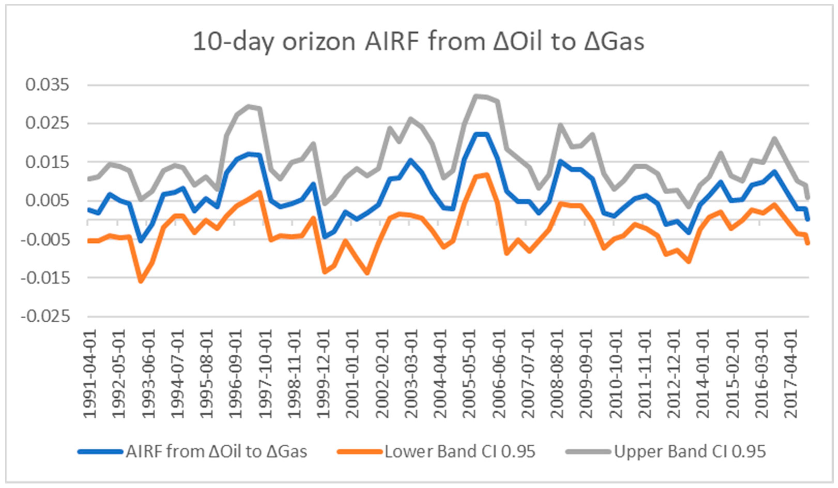
We report this kind of long term impacts with
Figure 7 and
Figure 8. When examining the long term impacts caused by gas to oil, we can reach the conclusion that gas returns have only insignificant accumulated impacts, as they are close to zero. An 1% shock to gas returns lead to less than 0.1% in oil returns change, as it marginally surpasses the 0.005%. The peaks almost coincide with the Granger test results, as gas returns only cause oil returns around 1/4/1998, 9/1/2004 and 9/10/2008 dates. As a matter of fact, we conclude that gas shocks are only short-lived to oil returns and without any magnitude. On the contrary, oil shocks cause larger long-term impacts to gas returns. Apart from three periods, where the impact is negative, the cumulative influence is always positive. Again we have long term impacts peaks, which agree with the periods of price spillovers presented by Wald tests. The largest impacts are around years 1996, 2003, 2006, 2008, 2009, 2014, and 2016. They are between 0.01% and 0.02%. The reason of the increased impact during those periods might be not coherent and attributed to different reasons, as some periods coincide with an evolving global financial crisis i.e., 2008 and 2009 affecting both markets, while some periods, i.e., 2014 and 2016 coincide with the application of an OPEC crude oil strategy to keep its market share and replace the shale production [
54]. Although the impact from oil to gas is higher, the level of impact cannot be perceived as high even in the above-mentioned periods, providing evidence on the decoupling of the markets.
Finally, we can reach the conclusion that gas has an extremely low long term impact on oil, while the long term impact from oil on gas is almost always positive and moves between 0.01% and 0.02%.
While we find negligible accumulated influence between 0.0000% and 0.0050% from gas to oil, Batten et al. [
17] find it up to 0.3000%. They find them also statistically significant and persistent. The calculated impulse of oil to gas by our study reaches the levels of 0.0250% while Batten’s et al. [
17] up to 0.4000%. The difference in magnitude implies the assumption of different character for the markets. Low impulses indicate highly liquid markets, while higher influences more tight. The low impact from one commodity to the other complies with Geng et al. [
16], who suggest that WTI impact on gas prices is fading. Since the ten-day horizon is short, then even more medium or long term impacts are negligible, something in further accordance with Geng et al. [
16]. Honarvar [
20] also finds low influence from one standard deviation of crude oil cost to unleaded retail premium gasoline price of 0.0100%.
4.5. Volatility Transmission
As discussed above, we also examine the volatility transmission, apart from the price spillovers. Even if one commodity might not affect the other commodity’s pricing, then it might affect the price range where the other commodity moves in. Volatility transmission might be more important, as it can shed light on whether these commodities can be used as hedging instruments against each other or for diversified and optimal portfolio allocation.
We start with our bivariate VAR (
Table 5), aiming to find evidence on volatility spillovers, as Singhal and Ghosh [
29] do for volatility spillovers between crude oil and market indices in India. We first account for serial correlation in our VAR model with the Portmanteau and Breusch-Godfrey statistics, and their results are negative (
Table 5). However, even from the
Figure 1 and
Figure 2, it is quite obvious that there is volatility clustering, i.e., periods of low volatility are followed by periods of high volatility. The ARCH LM test verifies our assumptions (
Table 5). We estimate that ΔGas
t−2 is statistically significant at 1%, and as a result transmits its volatility to oil. On the other hand, ΔOil
t−1 and ΔOil
t−4 are also significant at 5% and 10% respectively, when it comes to ΔGas volatility. Our first result again verifies that the true nature of volatility spillover is bilateral, and that no single commodity alone leads the market.
We estimate our DCC GARCH (1,1) coefficients as our data (returns) are stationary. We use both the symmetrical (DCC) and asymmetrical (ADCC) version of DCC GARCH (1,1) (
Table 6 and
Table 7). From our results, we can conclude there is statistical significance at 5% for our coefficients. Most importantly, the coefficients alpha and beta for both oil and gas are positive and significant. In addition, the sum of the coefficients for both commodities are close to one (1) implying that the shocks to the conditional variance are highly persistent. The sign and the sum, which is less than one (1), of alpha and beta coefficients for each commodity also validates the assumption of the stationarity of the covariance.
DCC GARCH models split volatility persistence of shocks on the dynamic conditional correlation into short and long-run components. Again, we have statistically significant coefficients for the symmetrical model, when the asymmetrical coefficient of the ADCC is not. Akaike criterion also suggests that the DCC is better fitting the data than the ADCC. The dynamic part of volatility comes from the DCCα whose value is close to 0.1, while the DCCβ is very close to 1. The magnitude of the two coefficients implies that there is a systematic correlation among the two commodities.
Figure 9 presents the time varying correlation between oil and gas in the US market. The correlation varies and it is not constant over time. By examining
Figure 1,
Figure 2 and
Figure 9, we can argue that correlation plummets between 2005 and 2009, which coincides with the period when oil reaches its lowest price, while gas price has a peak. The two prices follow a complete divergent course and this is why correlation is reduced. We have the same again phenomenon when correlation reaches low values during 2010, when the opposite happens, namely oil price advanced while gas price recessed. This result might imply that the shale revolution might have affected the volatility spillover, as low correlation implies more independent price fluctuations. Although markets are decoupled, the existence of bilateral volatility spillovers among the two commodities, as well as their substitutability, could be useful for diversified and optimal portfolio allocation. This is in alliance with similar results, examining the volatility transmission among crude oil and other sectors’ equity returns (Singhal and Ghosh, [
29]; Malik and Ewing [
13]).
To summarize, from the overall analysis undertaken in all
Section 4.1,
Section 4.2,
Section 4.3,
Section 4.4 and
Section 4.5, our paper contributes by updating the literature over the nature of the relationship among oil and gas prices with recent data, covering up to year 2017, using different econometric methodologies. From the analysis undertaken, the paper provides evidence of market decoupling for the whole period between the two commodities, which can help investors and policymakers adopt different strategies than before. Concerning the comparison of our work with recent studies, our results do not confirm the results of Batten et al. [
17] for the gas’ causality, neither that the two markets are decoupled, due to the shale revolution as Wakamatsu and Agura [
14] propose. Geng et al. [
15] and Geng et al. [
16], suggest that the US WTI and the Henry Hub prices were cointegrated before the sudden shale gas oversupply. We argue that for the examined period a certain threshold must be overpassed to have cointegration, as adjustment costs are not negligible. We further argue that the shale revolution has enhanced independence of the two markets, which was evident before the shale revolution. We agree with Wiggins and Etiene [
24], who conclude that demand elasticity is more elastic, since we can assume the possible substitution of the two commodities. Adding volumes in an already liquid market makes substitution even more feasible. Our results also do not confirm Atil et al. [
22] concerning their argument that natural gas adjusts to oil price changes. Finally, there are not persistent price spillovers, and when they are present their nature is bilateral, i.e., oil and gas can affect each other for short periods and without large magnitude.
5. Conclusions
The aim of research is to examine the time-varying price and volatility spillovers between the US crude oil and natural gas wholesale prices over the period 1990–2017, namely between the Henry Hub natural gas and the New York Mercantile Exchange (NYMEX) crude oil future prices. Our sample is consisted of 6975 observations of futures’ closing prices, as these prices adapt better the markets’ information and adjust faster than the spot markets. The paper contributes by updating the literature over the nature of the relationship among oil and gas prices with recent data, covering up to year 2017, using different econometric methodologies. The main finding of the paper is that we provide evidence of market decoupling between oil and gas in the US wholesale market for the whole period. We further argue that the shale revolution has enhanced independence of the two markets, which was evident before the shale revolution.
We examined several aspects of the price and volatility spillovers. We examine the presence of causal relationship with Wald tests, the out-of-sample predictive ability for full sample periods and shorter iterations between the two commodities, the asymmetric price transmission, the long-term price impacts and the time-varying volatility transmission among the commodities. We apply several econometric methodologies to derive conclusions: Bivariate vector autoregression (VAR) models assuming that oil and gas price variables are endogenous allowing feedback between prices, the Momentum Threshold Autoregressive (MTAR) cointegration for examining asymmetric relationships between prices, out of sample Granger causality tests with Diebold and Mariano forecasting accuracy test, accumulated impulse response functions (AIRF) to examine long-term price relationships, and Dynamic Conditional Covariance (DCC) GARCH model to elaborate volatility transmission.
We conduct Wald tests for the full sample and for shorter periods, representing periods of a single year. Wald tests are symmetrical, meaning that they consider a potential increase of the first commodity will have of the same magnitude and speed of adjustment effect as a decrease. Initially, we find weak evidence of a unilateral causality from natural gas to oil for the full sample period. When we test for shorter iterations we find that there are periods when causality from gas to oil and vice versa exist, but these periods are very few and short-lived, considering the over 28-year period we examined. In most of the years they follow different and independent paths.
With the asymmetric price transmission analysis, we find evidence of positive asymmetry from crude oil to natural gas prices i.e., oil price increases cause faster adjustments to natural gas prices than oil price decreases. The positive spatial asymmetry, as we considered both markets as individual and separately operational, provides evidence that traders absorb information faster from price increases than decreases.
With the out of sample analysis, we can validate that the inclusion of the second’s commodity coefficients does not improve the predictive ability of our models meaning that the two commodities remain largely independent. There is only one year (1999), when we find causality from oil to gas, but this is not sufficient enough to alter our general conclusions of decoupled markets.
To elaborate the long-term impacts analysis, we consider two trading weeks—i.e., 10 days. This is due to the fact that we refer to highly liquid markets with intensive information absorption. We reach useful results when we calculated the 1% price shock of one commodity’s long term impact to the other’s price, where the accumulated long term impact that gas price changes have to oil is close to zero, as it surpasses the 0.005% level only three times and lasts for very short periods. On the contrary, 1% of oil price change causes positive gas price reactions between 0.01% and 0.02%.
The volatility transmission analysis shows that bidirectional volatility spillovers are evident and are mainly attributed to the long term component, rather than the dynamic one. There is a systematic correlation between the two commodities, but this is time varying. As a consequence, this confirms that the commodities follow two different market determined courses. The commodity independence can be asserted by the increased liquidity and financialization of the US markets. There is an increased number of participants trading high volumes and these volumes change hands many times leading to a high churn ratio. The transparency of NYMEX exchange enhances the decoupling between the two markets.
From the whole analysis, our main contribution to the literature is that we provide evidence of market decoupling between oil and gas in the US wholesale market, using data over the period 1990–2017. The result of two decoupled markets has great implications for both investors and policy makers. The fact that markets are decoupled, and that each commodity’s volatility cannot be easily predicted through the other’s volatility, leads to the conclusion that each commodity cannot be perceived as a perfect hedging instrument for the other. However, the bidirectional volatility transmission among the two commodities and their substitutability could be useful for diversified and optimal portfolio allocation, based on the assumption of two independently evolving markets. This is in alliance with similar results, examining the volatility transmission among crude oil and other sectors’ equity returns.
Markets are decoupled throughout the whole period, as there is either gas oversupply or high inventories. The present situation, with no spillovers between the markets, may be reversed if gas exports prevail, removing substantial excess quantities from domestic natural gas market. Another factor that could enhance the re-linkage among the two commodities is that of the high demand, which could make the present infrastructure insufficient. Since the US gas pricing is determined more based on market fundamentals, compared to other regional gas markets, i.e., there exist no long-term oil-indexed gas pipeline contracts, traders do not have the option to use one commodity as a financial instrument for hedging purposes.
Our analysis provides insights in the price and volatility spillovers; however it could be further enhanced. A limitation in our analysis is the consideration of rolling periods of 250 datapoints, as the effect of any potential structural break proved to be not statistically significant. The consideration of other rolling period could capture the impact of the transitionary effects. This could be the case of shorter rolling periods, while in case of the adoption of higher rolling periods might lead to misleading results, as longer time periods could probably be better examined with other methodological approaches, i.e., regression analysis incorporating other variables.
A potential extension of our analysis is the examination of other markets, such as the National Balancing Point (NBP) and/or the Title Transfer Facility (TTF) prices concerning gas markets and the Brent price of the Intercontinental Exchange (ICE) concerning oil markets in Europe, or the Japan Korea Marker (JKM) prices and the Japan Customs-cleared Crude (JCC) prices concerning the gas and oil markets in Asia respectively. The examination of different regions could provide useful insights concerning the maturity of each regional market. This could further enhance the policymakers to can take advantage of the conclusions and design fully integrated markets at regional and global level. For example, one pillar of European Union’s Energy Union is that of a fully functional and integrated gas market. Economists can compare the prevailing conditions in more mature markets and better understand the consequences for markets integration.


