Abstract
In this paper, a Frequency-Dependent Pi Model (FDPi) of a three-core submarine cable is presented. The model is intended to be used for the representation of submarine cables in an Offshore Wind Power Plant (OWPP) scenario for both time and frequency domain analysis. The frequency-dependent variation of each conductive layer is modeled by a Foster equivalent network whose parameters are tuned by means of Vector Fitting (VF) algorithm. The complete formulation for the parameterization of the model is presented in detail, which allows an easy reproduction of the presented model. The validation of the model is performed via a comparison with a well-established reference model, the Universal Line Model (ULM) from PSCAD/EMTDC software. Two cable system case studies are presented. The first case study shows the response of the FDPi Model for a three-core submarine cable. On the other hand, the second case study depicts the response of three single-core underground cables laying in trefoil formation. This last case shows the applicability of the FDPi Model to other types of cable systems and indirectly validates the response of the aforementioned model with experimental results. Additionally, potential applications of the FDPi model are presented.
1. Introduction
Increasing construction of Offshore Wind Power Plants (OWPPs) has been accompanied by a progressive installation of submarine cables in the power system [1]. Since these type of cable networks are affected by many transient phenomena (frequent load changes, switching operations, etc.) and harmonics that can be amplified by cable resonances, proper modeling of submarine cables is crucial in order to perform an adequate analysis of their behavior and their effects on the power system.
State of the art time domain models of power cables take into account the frequency dependency of the physical parameters in order to enable accurate transient simulations [2]. Due to their formulation, these models cannot be directly converted into the Laplace domain or in a state-space form, in order to analyze the stability and the frequency response of the power system under study. Thus, submarine cables are commonly represented in power system stability studies by cascaded traditional Pi sections that neglect the frequency-dependent effects [3]. This way of modeling is unable to accurately represent the damping characteristic of the cable and can lead to incorrect results and analysis [4].
Regarding this issue, several contributions have been done in order to improve the damping characteristic of the traditional Pi model. In general terms, these contributions consist of including the inductive coupling between the cable layers (core and screen) [5] or by including equivalent networks that represent the variation in frequency of the cable parameters [4,6]. The model proposed in reference [4] eliminates the contribution of the cable screens by assuming them to be at ground potential (even though they might not be grounded at both ends). On the contrary, references [6,7] represent a cable system with a Pi equivalent circuit including the frequency dependence of the cable longitudinal impedance in the modal domain. For this model approach, transformations between both domains, phase and modal, are required.
This paper presents an alternative Frequency-Dependent Pi (FDPi) Model that represent reasonably well the steady state and transients comprising frequencies up to 10 kHz but can be extended to higher frequencies if required. The model consists of cascaded Pi sections, which incorporate both inductive coupling and the frequency dependent characteristic of some series impedance terms of the conductive layers.
The strengths of the presented model in comparison to other published model contributions lie in the following points:
- The model represents each cable conductive layer, thus not assuming the elimination of the cable screens and external wire armour, which allows the visualization of the voltages and currents of these conductors and the representation of different grounding configurations. Furthermore, it is possible to account for the frequency dependency of the earth-related terms by explicitly representing the earth as another conductor [8,9].
- The model is explicitly represented in the phase domain, thus avoiding the transformation between phase domain to modal domain and vice versa.
- The model can be directly formulated in the Laplace domain or in a state-space representation. Thus allowing different studies oriented to frequency analysis, stability, sensitivity to parameter deviation, participation factors of the system’s variables, and others. Backward Euler method, or other techniques presented in reference [10], can be used in order to compute the voltages and currents along the cable in the time domain. In this sense, both time and frequency domain analysis can be performed.
- The model can be easily implemented in Matlab/Simulink or any other circuit simulation tool by means of discrete RLC components. Coupled resistances and inductances are directly implemented by means of a generalized mutual inductance component. Time domain simulations of the submarine cable model can be performed directly by selecting a solver option and a sample time. Typical solver methods available in simulation tools are Backward Euler, Trapezoidal Rule and Runge-Kutta.
- The modeling approach is not only applicable to three-core submarine cables. It can be extended to other types of cable systems, such as single-core underground and submarine cables or a set of single-core cables arranged in flat or trefoil formation.
In this sense, the FDPi model presented in this paper is intended to be in use with the Wind Turbine Harmonic Model presented in reference [11] and other power component models (such as transformers, filters, etc.) for the analysis and study of an OWPP. The studies can be oriented towards design aspects, harmonic assessment, stability studies, frequency analysis, and others.
The paper is structured as follows: Section 2 introduces the electrical schematic and the general equations that describe the behavior of the FDPi model. Section 3 presents the parameterization of the model. A detailed description of the formulation is presented in this section, which allows an easy reproduction of the model and the case studies without the need of resorting for additional information. Section 4 treats the validation of two case studies, a three-core submarine cable and three single-core underground cables laying in trefoil formation. The validation of the FDPi model is performed via a comparison of the proposed model with the well-established Universal Line Model (ULM) from PSCAD/EMTDC software. Section 5 provides a methodology for the determination of a suitable order of the proposed model. The order of the FDPi model is highly dependent on the accuracy and frequency range requirements and the intrinsic characteristics of the cable system. Section 6 introduces the potential applications of the proposed FDPi model. Finally, conclusions about the presented model and the obtained results are detailed.
2. Frequency-Dependent Pi Model
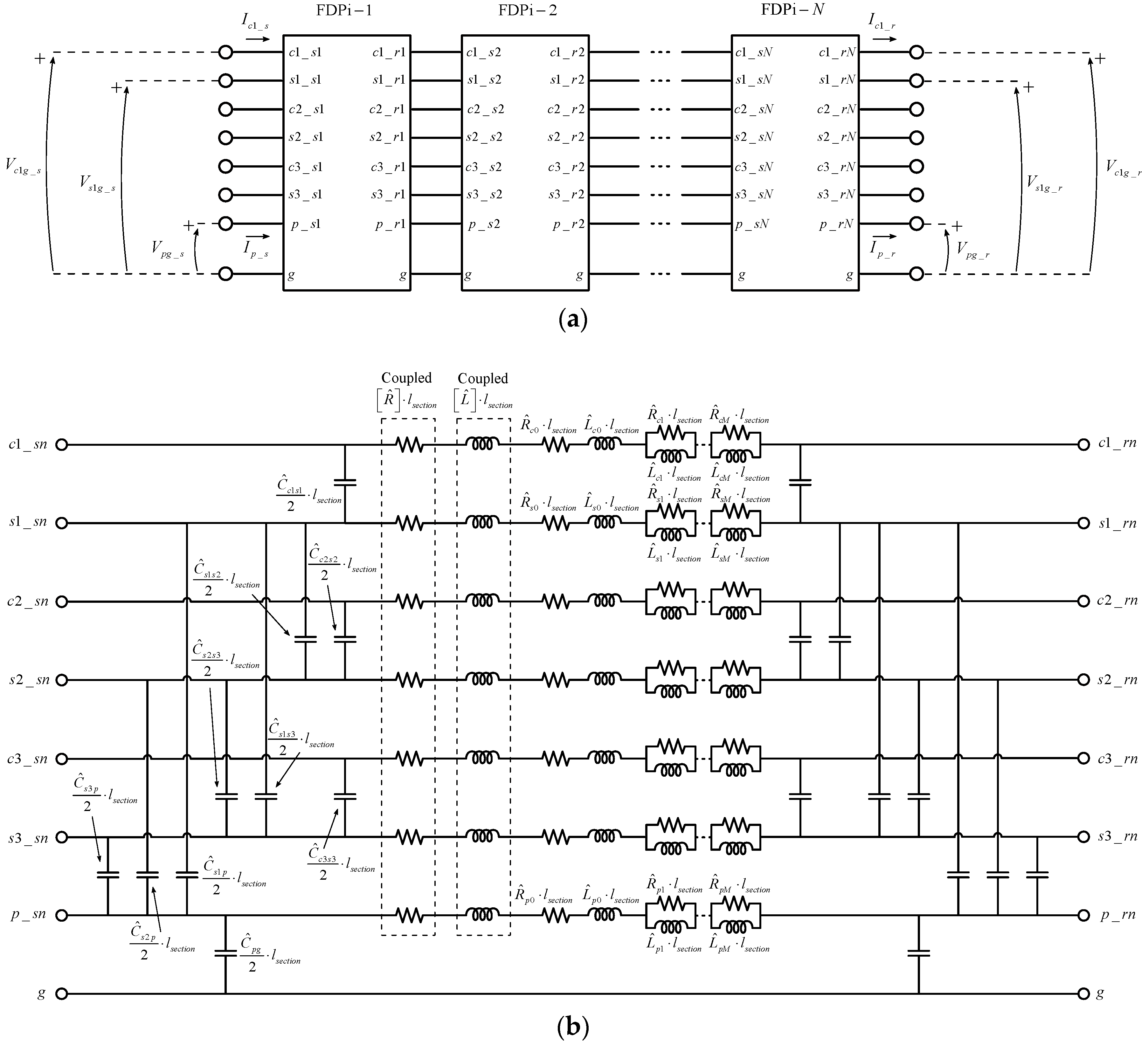
Figure 1 shows the electrical schematic of the FDPi Model. The model physically represents the seven conductors of a three-core submarine cable system: three core conductors, three screen conductors and a pipe representing the external wire armour of the cable.

Figure 1.
Electrical schematic of the Frequency-Dependent Pi (FDPi) Model. (a) Cascaded FDPi sections. (b) Detailed schematic of an FDPi section (Capacitances at the right-hand side are equal to the left-hand side, but their names are omitted for simplicity).
As depicted in Figure 1a, the model consists of N cascaded FDPi sections. Each FDPi section consists of a coupled resistance and inductance matrix computed at the nominal frequency, 50 Hz or 60 Hz. The capacitive coupling between conductors is computed at the nominal frequency as well. The frequency dependent behavior of the series impedance terms of each conductive layer is represented by means of a Foster equivalent network as depicted in Figure 1b.
The order of the FDPi model is given by the number of cascaded sections (N) together with the order of the Foster equivalent networks (M). The order of the model is chosen depending on the cable length, accuracy and frequency range requirements.
The general equations that describe the behavior of the model are expressed in the Laplace domain (). The terminal voltages and currents of the FDPi model are given by Equation (1). Being , the identity matrix of order seven.
The voltages and currents at the sending and receiving ends are vectors defined by Equation (2). Each voltage is referenced to ground potential as depicted in Figure 1:
The series impedance matrix and the shunt admittance matrix are given by Equations (3) and (4), respectively:
The length of a Pi section is given by Equation (5), where is the total length of the cable:
The per-length unit series impedance matrix is given by Equation (6):
Being matrix defined by Equation (7):
The matrix includes the contribution of the Foster equivalent networks of each conductive layer (cores, screens and armour) and is given by Equations (9)–(13):
The per-length unit shunt admittance matrix is defined by Equation (14):
being:
The per-length unit capacitances between conductors (depicted in Figure 1b) are given by the following equations:
The capacitances to ground for each cable conductor (cores, screens and armour) are computed according to the following equations:
The capacitances of Equations (19)–(21) are zero because of the physical structure of the cable. Therefore, they are not represented in the schematic of Figure 1b. The rest of the capacitance elements presented in Equation (15) and not named previously are zero as well. Supporting information about the capacitance matrix of Equation (15) is presented in [12].
3. Model Parameterization
The frequency-dependent variation of the electrical parameters of a cable system is due to skin effect and proximity effect. There are several methods proposed in the technical literature for determining the electrical parameters of a cable system and their variations with frequency. The most remarkable techniques are based on analytical formulas [13,14,15], numerical tools based on Finite Element Method (FEM) [16,17], conductor partitioning [18,19] and the Method of Moments (MoM-SO) proposed in [20,21,22]. Each technique has its advantages and disadvantages in terms of complexity, accuracy, computational time, phenomena that represent and other aspects.
In this paper, the analytical equations, presented in reference [13], are used for the parameterization of the model. The main reason for its selection is that most Electromagnetic Transient (EMT) tools use this formulation to compute the electrical parameters of the cable. Therefore, this way of parameterization is followed in order to compare the behavior of the FDPi model with a reference model, Universal Line Model (ULM) from PSCAD/EMTDC software. It is worth to mention, that the analytical equations, addressed in reference [13], only take into account the skin effect and do not consider the proximity effect. If it is required to consider the proximity effect, the methodology presented in reference [14] and other special methods already mentioned above such as FEM, conductor partitioning and MoM-SO can be used for model parameterization.
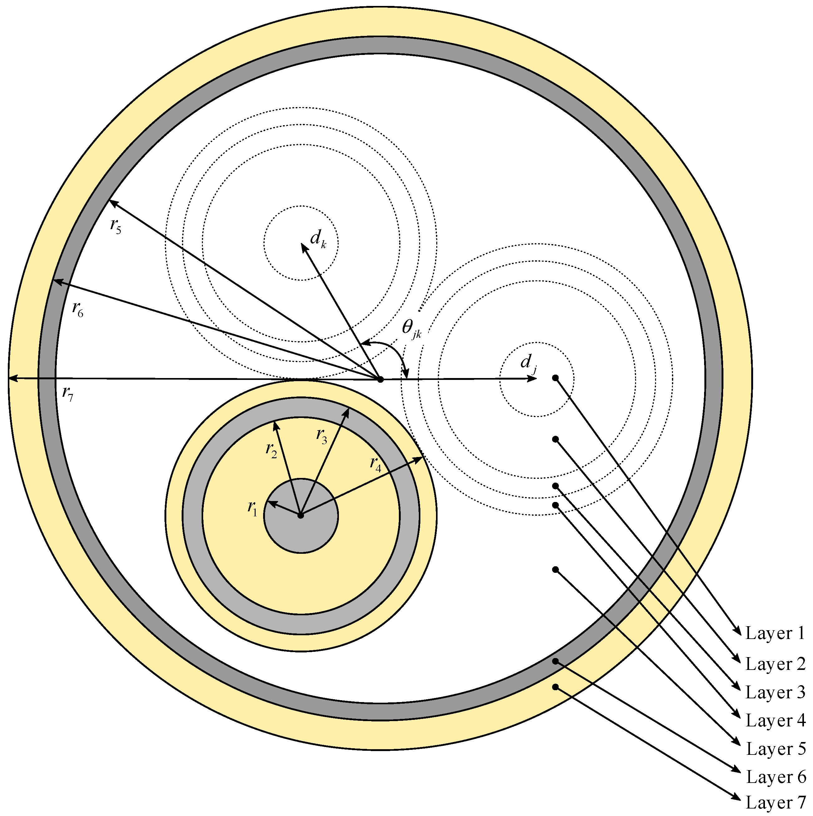
In order to perform the cable parameterization according to the analytical equations, it is necessary to perform a data conversion of the original cable parameters into a new set of parameters. This new set of parameters consists in the simplification of the cable layers and in the correction of the materials properties. Details of the conversion procedure can be found in references [23,24]. Figure 2 shows the simplified cross-section of the cable under study. Table 1 gives information about the required set of parameters.

Figure 2.
Simplified cross-section of a three-core submarine cable.

Table 1.
Simplified layers of a three-core submarine cable.
The determination of the electrical parameters of the FDPi model involves three steps, which are described in the next subsections in order to allow an easy reproduction of the model.
3.1. Computation of and Matrices
For the determination of the resistance and inductance matrices, the per-length unit series impedance matrix is computed at the nominal frequency and is given by Equation (23):
The cable internal impedance matrix is given by Equation (24):
being:
The series impedance of the core insulation is given by Equation (28):
The screen inner and outer series impedance are given by Equations (29) and (30), respectively:
being:
- Bessel function of x, of first kind and order n.
- Bessel function of x, of second kind and order n.
The series impedance of the screen insulation is given by Equation (32):
The screen mutual series impedance is given by Equation (33):
The pipe internal impedance matrix is defined by Equation (34):
being:
The mutual impedance matrix between pipe inner and outer surfaces is given by Equation (41):
being:
The pipe outer series impedance is given by Equation (43):
The series impedance of the pipe outer insulation is given by Equation (44):
The pipe mutual series impedance is given by Equation (45):
Finally, is a square matrix of order seven that represents the earth-return impedance. This impedance term can be defined by Saad’s approximation, Equation (46):
being:
Once all previous terms are calculated, the matrix is computed at nominal frequency and the and matrices can be obtained by splitting real and imaginary parts, as given by Equations (7) and (8).
3.2. Computation of Foster Equivalent Networks
For the computation of the Foster equivalent networks shown in Figure 1b, a frequency sweep is done to , and terms. The series impedance of the core conductor is given by Equation (48):
being:
and terms are defined in Equations (30) and (43), respectively. Table 2 shows the general data that is needed to obtain the Foster equivalent networks. The frequency vector is mainly defined in dependence of the frequency range of interest.
Table 2.
Required general data for the determination of the Foster equivalent networks.
The frequency-dependent behavior for each series impedance term is approximated by means of Vector Fitting (VF) algorithm [25,26,27]. VF provides an adequate representation of the series elements in the frequency domain by means of a rational function on pole residue form, as given by Equation (50):
The rational function, obtained from the fitting process, is represented by a Foster equivalent network of order M, as depicted in Figure 3. The order of the equivalent network depends mainly on the frequency range and accuracy requirements.
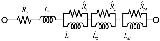
Figure 3.
Foster equivalent network of order M.
The electrical parameters of the Foster equivalent network are given by Equation (51):
It is possible to incorporate the and terms, calculated for each conductive layer (core, screen and pipe), into the main diagonal of the and matrices of Equation (7). In this way, a reduction in the number of components shown in Figure 1b can be performed, leading to a more practical model and improving the computational load due to a lower number of components.
3.3. Computation of Matrix
The per-length unit shunt capacitance matrix is computed at the nominal frequency from the potential coefficient matrix , as given by Equations (52) and (53):
The cable internal coefficient matrix is given by Equation (54):
being:
The pipe internal coefficient matrix is given by Equation (57):
being:
The potential coefficient matrix between pipe inner and outer surfaces is a square matrix of order seven with all its elements given by Equation (60):
As already shown, the above procedure details the steps and the formulation required for model parameterization.
4. Validation Case Studies
This section introduces two numerical case studies in order to validate the model of Figure 1. The FDPi model is directly implemented in Simscape Electrical (Matlab/Simulink) and the Backward Euler technique is chosen as solver method for time domain computations.
4.1. Case Study #1: Three-Core Submarine Cable
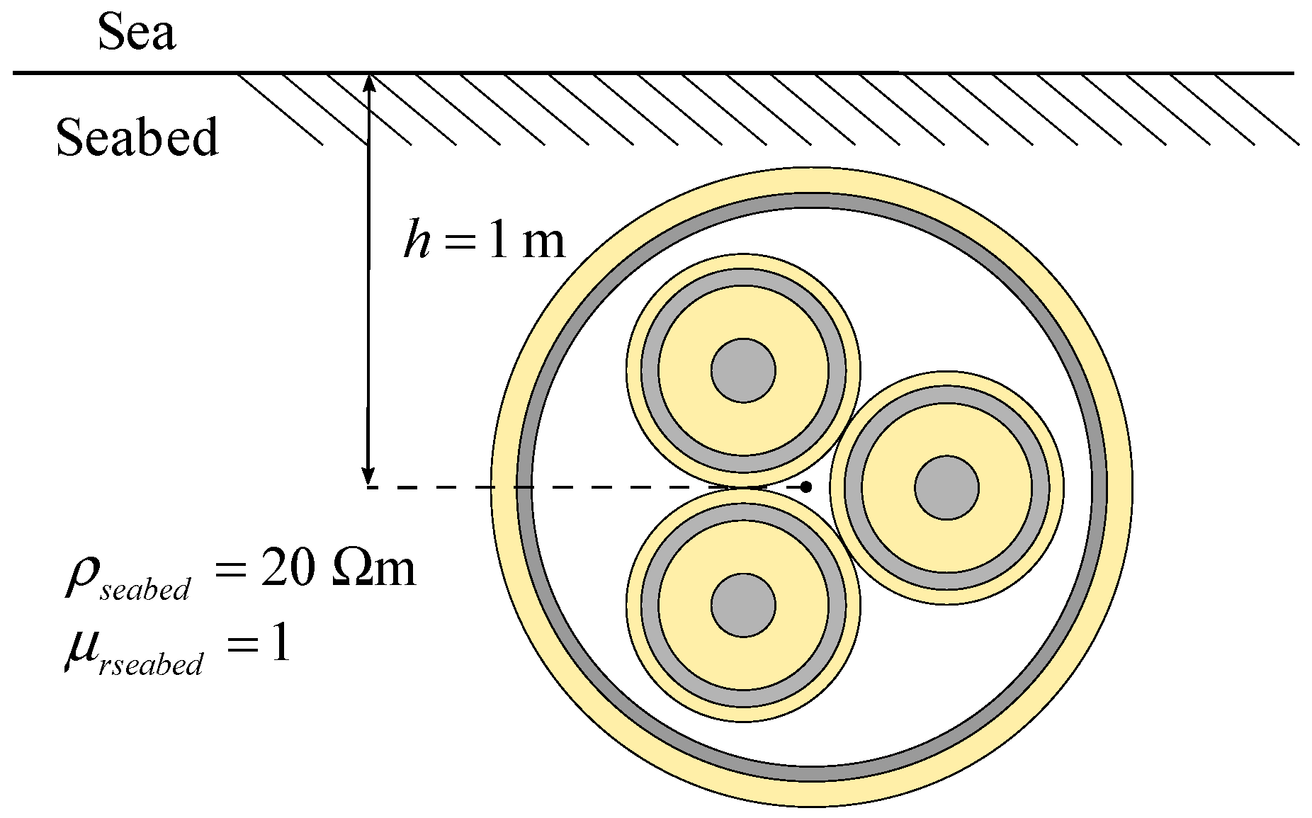
This case study consists of a buried three-core submarine cable. Figure 4 shows the simplified cross-section of the submarine cable under study and gives information about the surrounding medium properties and burial depth of the cable. The required geometrical and material properties of the cable are listed in Table 3. The information presented in Figure 4 and Table 3 is adopted from [22,28].
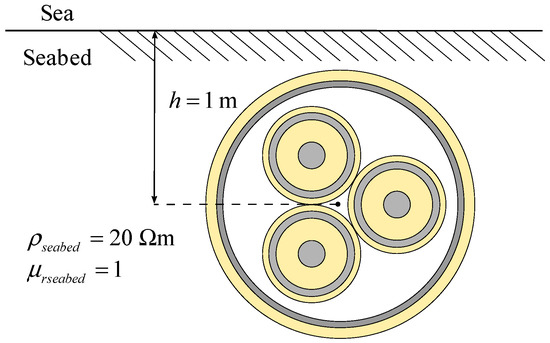
Figure 4.
Cable cross-section for Case Study #1 and installation conditions (laying depth and surrounding medium properties).
Table 3.
Geometrical and material parameters for Case Study #1.
The requirement of the validation is to represent the steady state and transients comprising frequencies up to 10 kHz, which is the frequency range of interest for the studies mentioned at the end of Section 2 and in Section 6. To fulfill this objective, the FDPi model is built with 32 cascaded FDPi sections (N = 32), each one with Foster equivalent networks of order three (M = 3) for each conductive layer term. The series impedance terms were fitted for a frequency range from 0.1 Hz up to 10 kHz by means of VF algorithm.
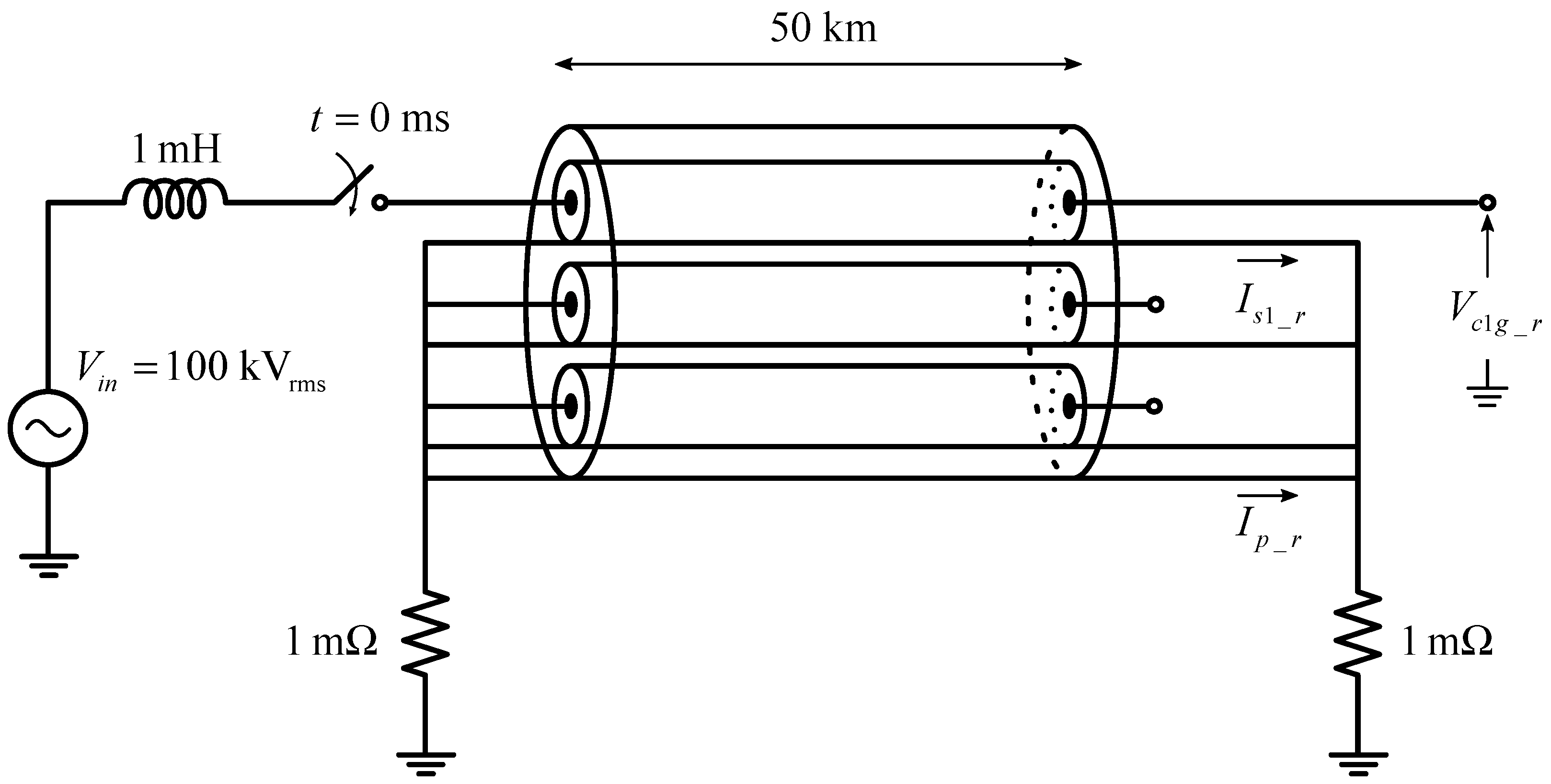
In order to validate the FDPi model in the time domain, the test configuration of Figure 5 has been used considering a cable length of 50 km. The test is as proposed in references [29,30]. The test consists of energizing one-phase of the cable with an AC voltage source at its sending end and with the receiving ends open. The input source signal is a cosine function with a nominal voltage of 100 kVrms. The energization takes place at the peak voltage of the input source in order to produce the highest transient current.
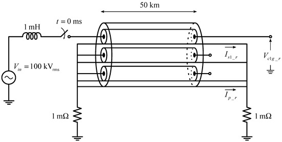
Figure 5.
Setup for time response validation—Case Study #1.
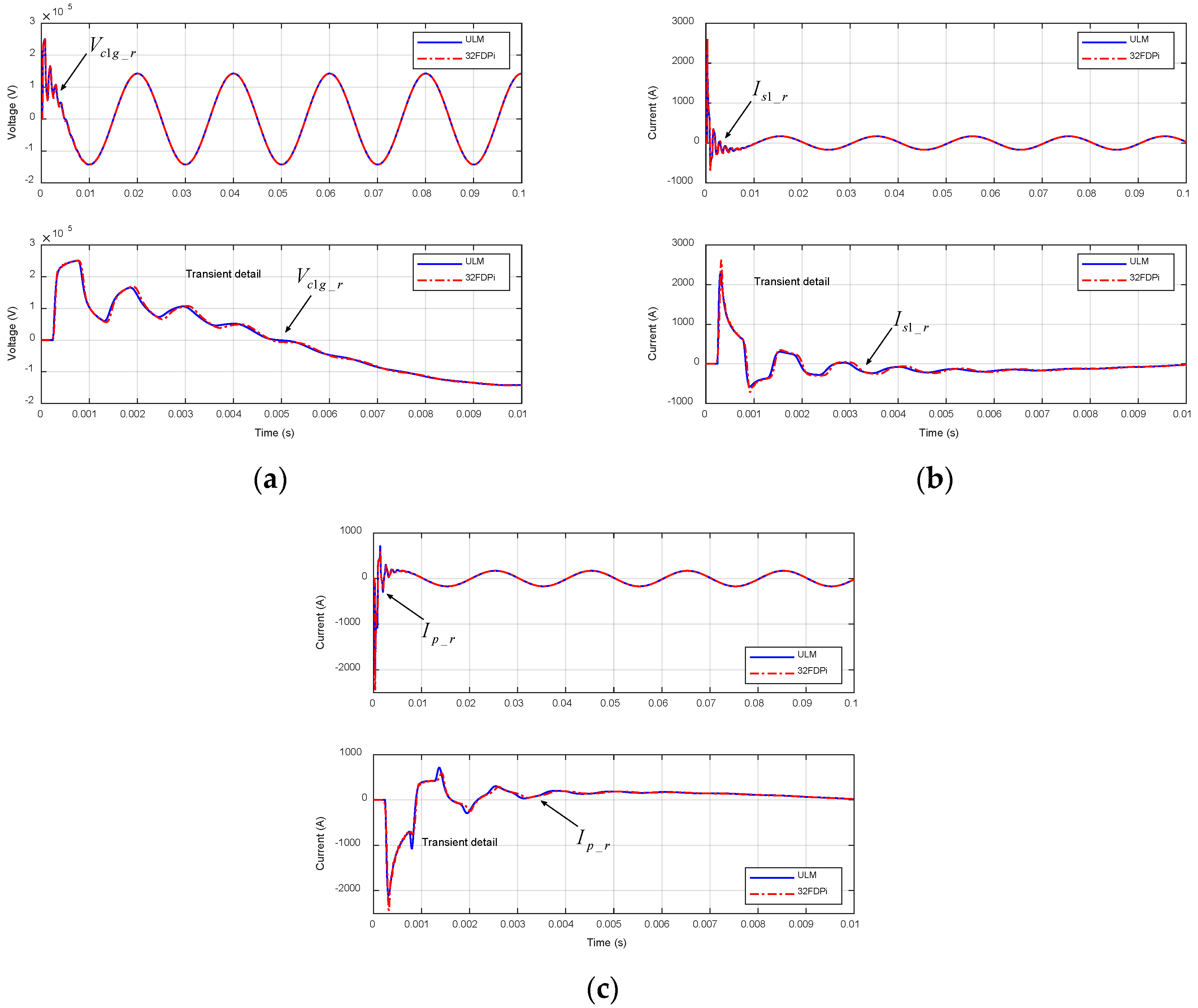
Figure 6 shows the time domain response of the receiving end signals depicted in Figure 5. Each graphic shows information about the steady state and transient state (top one) and a zoom in for the first 10 ms (down one) in order to show the transient response in detail.
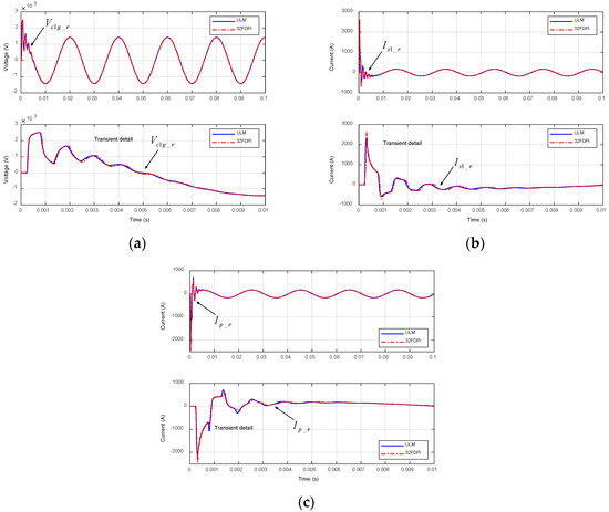
Figure 6.
Time response comparison for Case Study #1. (a) Vc1g_r. (b) Is1_r. (c) Ip_r.
As depicted in Figure 6, the results of the FDPi model show a very good agreement with the ones obtained from the reference model. The shape and amplitude of the time signals are very similar and a good representation of the wave travel time is performed by the FDPi model.
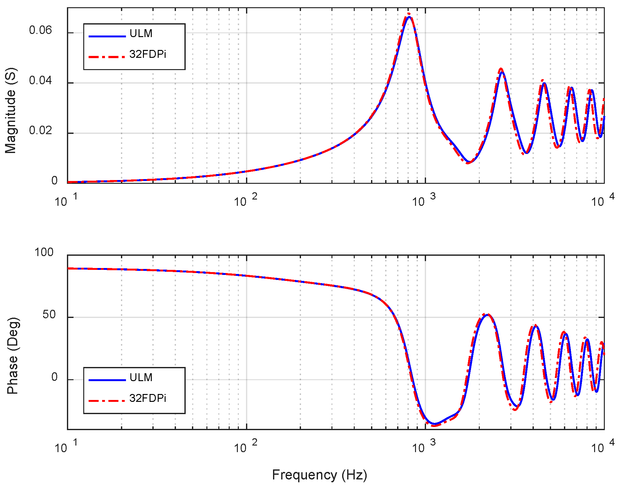
Figure 7 shows the magnitude and phase of the cable admittance. As indicated for the signals in the time domain, the admittance of the cable (magnitude and phase) is very similar for both models up to a frequency value of 10 kHz.
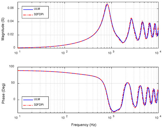
Figure 7.
Cable admittance comparison for Case Study #1.
The short deviation of the FDPi model with respect to the reference model is due to four main reasons. First, the parameterization that is performed by the ULM model from PSCAD/EMTDC software is not exactly the same as in reference [13]. Therefore, the comparison of both models is performed with slightly different parameter values.
Second, the representation of the FDPi model is built in order to consider frequencies up to 10 kHz. The error of the model can be reduced by considering a higher frequency range. In order to do this, the order of the model has to be increased but at the expense of increasing the computational cost.
Third, the FDPi model only takes into account the frequency dependency of the series impedance terms , and . The frequency dependent behavior of other terms is not taken into account.
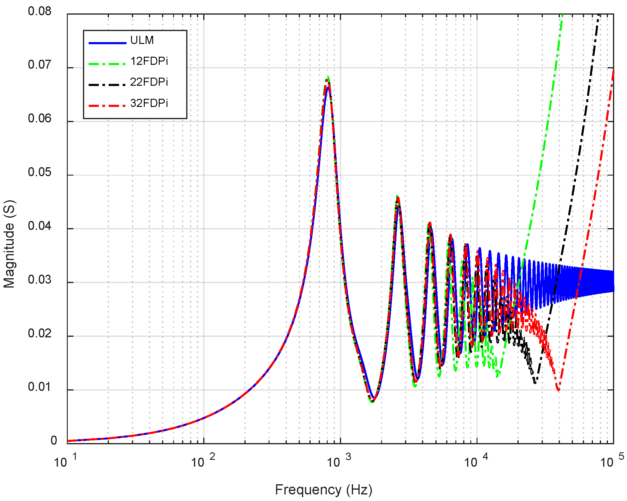
Finally, an additional oscillation is presented in the results of the FDPi model due to the nature that lumped parameters models introduce an unreal resonance, as explained in reference [31]. Is in fact, a resonance that is not present in the real cable but that appears because of the model characteristics. In order to show this unreal resonance, Figure 8 depicts the cable admittance for a frequency range of 100 kHz. It can be seen that for the FDPi model order (M = 3 and N = 32) considered previously, the unreal resonance is located around 40 kHz and with a magnitude of 0.01 Siemens.
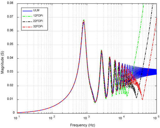
Figure 8.
Cable admittance comparison for Case Study #1 with different number (N) of cascaded FDPi sections.
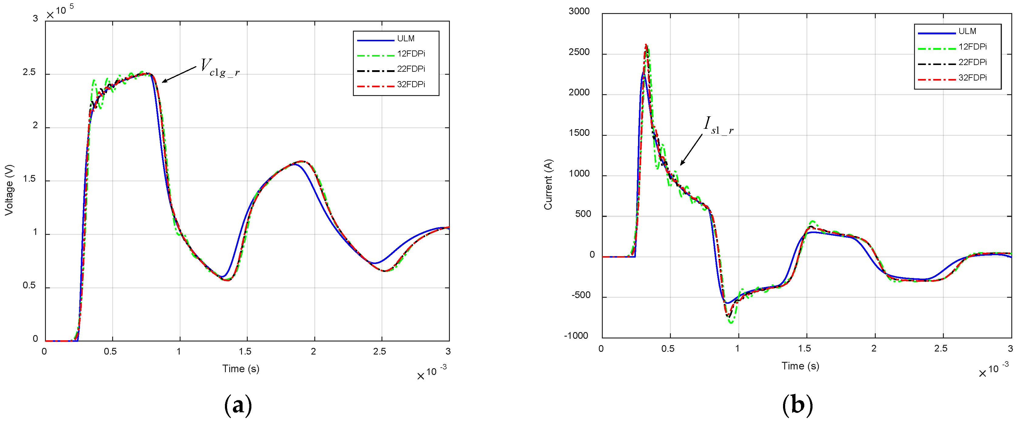
Figure 8 also performs an evaluation of different number (N) of cascaded FDPi sections while keeping the same order of Foster equivalent networks (M = 3). Two important aspects can be inferred from Figure 8:
- An increase in the model order allows extending the frequency range of the model, which gives a lower deviation in time and frequency domain results.
- The unreal resonance is shifted to the right in frequency and decreased in magnitude by increasing the model order.
Figure 9 shows the impact of the model order on the time signals. It can be seen that for lower model orders there is a higher oscillation magnitude.
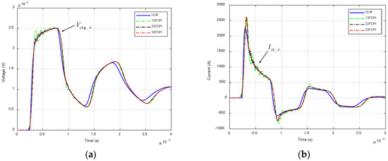
Figure 9.
Time response comparison with different number (N) of cascaded FDPi sections for Case Study #1. (a) Vc1g_r. (b) Is1_r.
4.2. Case Study #2: Single Core Underground Cable
The cable system for this second case study consists of three single core cables (one for each phase) as depicted in Figure 10. This figure shows the simplified cross-section of each single core cable and gives information about the surrounding medium properties, burial depth and laying formation of the cable system.
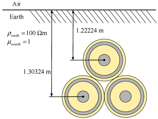
Figure 10.
Cable cross-section for Case Study #2 and installation conditions (laying depth and surrounding medium properties). Source [31].
Each single core underground cable operates with a nominal voltage of 150 kV. The cable has a core cross-section of 1200 mm2 and its insulation material is XLPE (cross-linked polyethylene).
The required geometrical and material properties of the cable are listed in Table 4. The information presented in Figure 10 and Table 4 is adopted from [31].
Table 4.
Geometrical and material parameters for Case Study #2. Source [31].
As in the previous case, the requirement of the validation is to represent the steady state and transients comprising frequencies up to 10 kHz. To fulfill the objective the FDPi model is built with 35 cascaded FDPi sections (N = 35), each one with Foster equivalent networks of order three (M = 3) for each conductive layer term. The series impedance terms were fitted for a frequency range from 0.1 Hz up to 10 kHz by means of VF algorithm.
In order to validate the response of the FDPi model in the time domain, the test configuration of Figure 11 has been used considering a cable length of 50 km. Similar to the previous case, the test consists of energizing one-phase of the cable with an AC voltage source at its sending end and with the receiving ends open. The input source signal is a cosine function with a voltage magnitude of 150 kVrms (nominal voltage given by the cable manufacturer). The energization takes place at the peak voltage of the input source in order to produce the highest transient current.
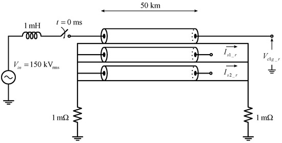
Figure 11.
Setup for time response validation—Case Study #2.
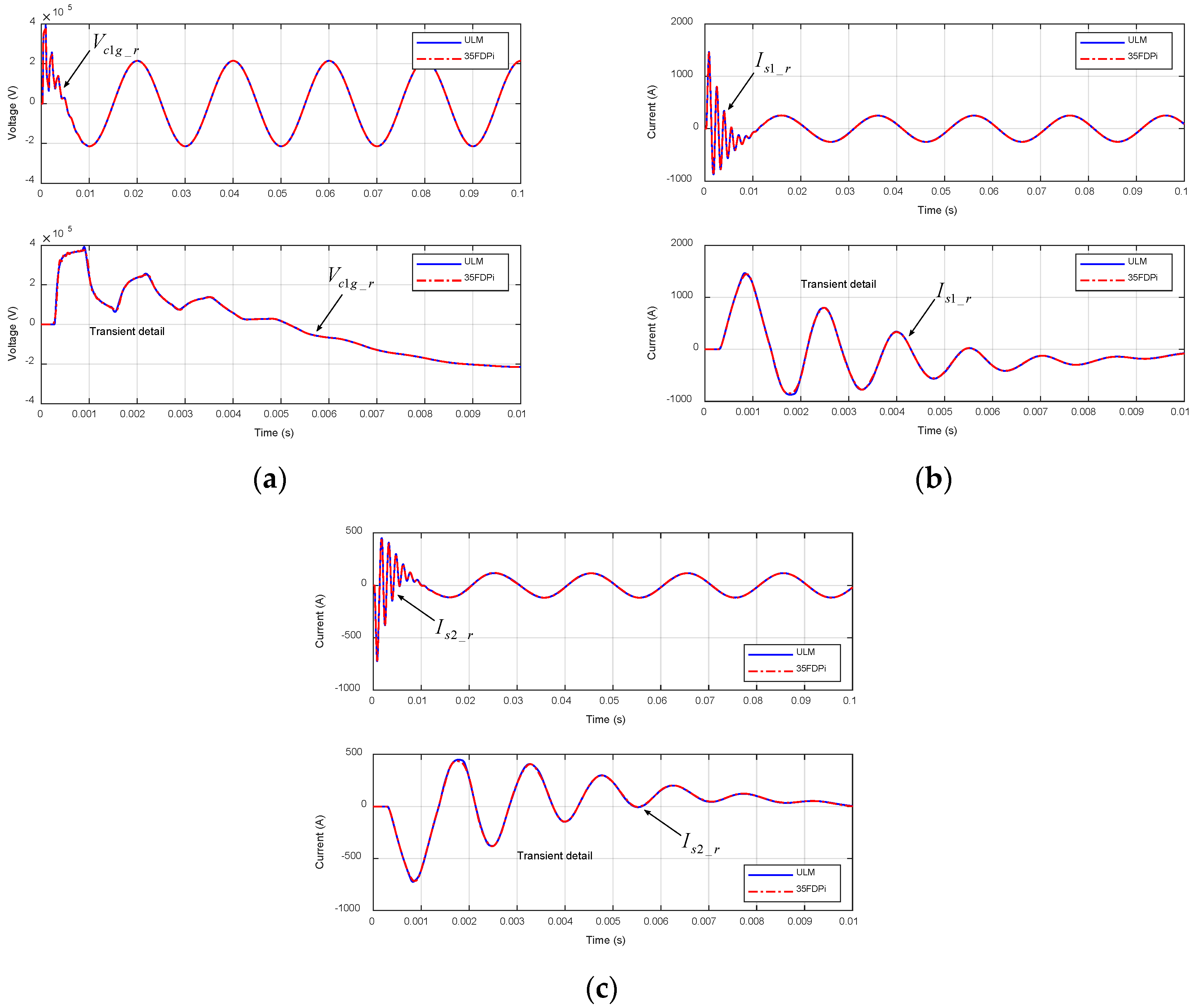
Figure 12 shows the time domain response of the receiving end signals (depicted in Figure 11) for the Case Study #2. As in the previous case, each plot shows information about the steady and transient state (top one) and a zoom in for the first 10 ms (down one) in order to show the transient response in detail.
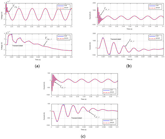
Figure 12.
Time response comparison for Case Study #2. (a) Vc1g_r. (b) Is1_r. (c) Is2_r.
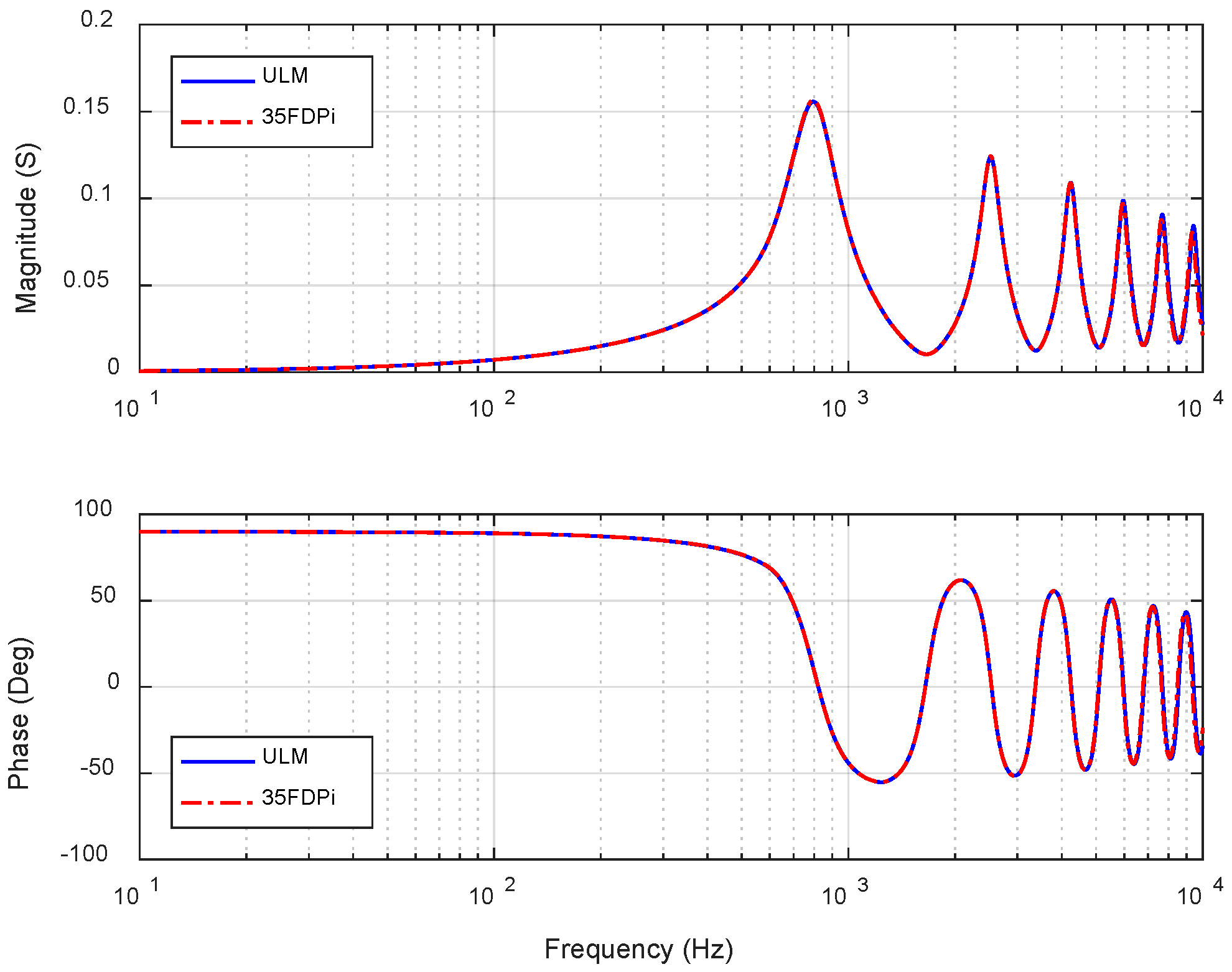
Figure 13 shows the magnitude and phase of the cable admittance for a frequency range of 10 kHz.
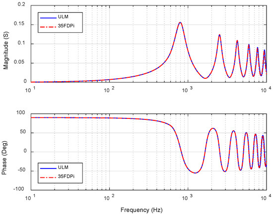
Figure 13.
Cable admittance comparison for Case Study #2.
As depicted in the previous figures, time and frequency domain results obtained from the FDPi model show a very good agreement with the ones obtained from the reference model. The shape and amplitude of the time signals are very similar and a good representation of the wave travel time is obtained by the FDPi model. Furthermore, it can be seen that the results obtained for this case study present a lower deviation in comparison with the previous one.
This lower deviation is mainly because the formulation used for cable parameterization (single core cables) is the same as the one used by the ULM model from PSCAD/EMTDC software. Therefore, the same values for the series impedance terms and shunt admittance terms are obtained and the differences in the results are mainly due to the characteristics of both models.
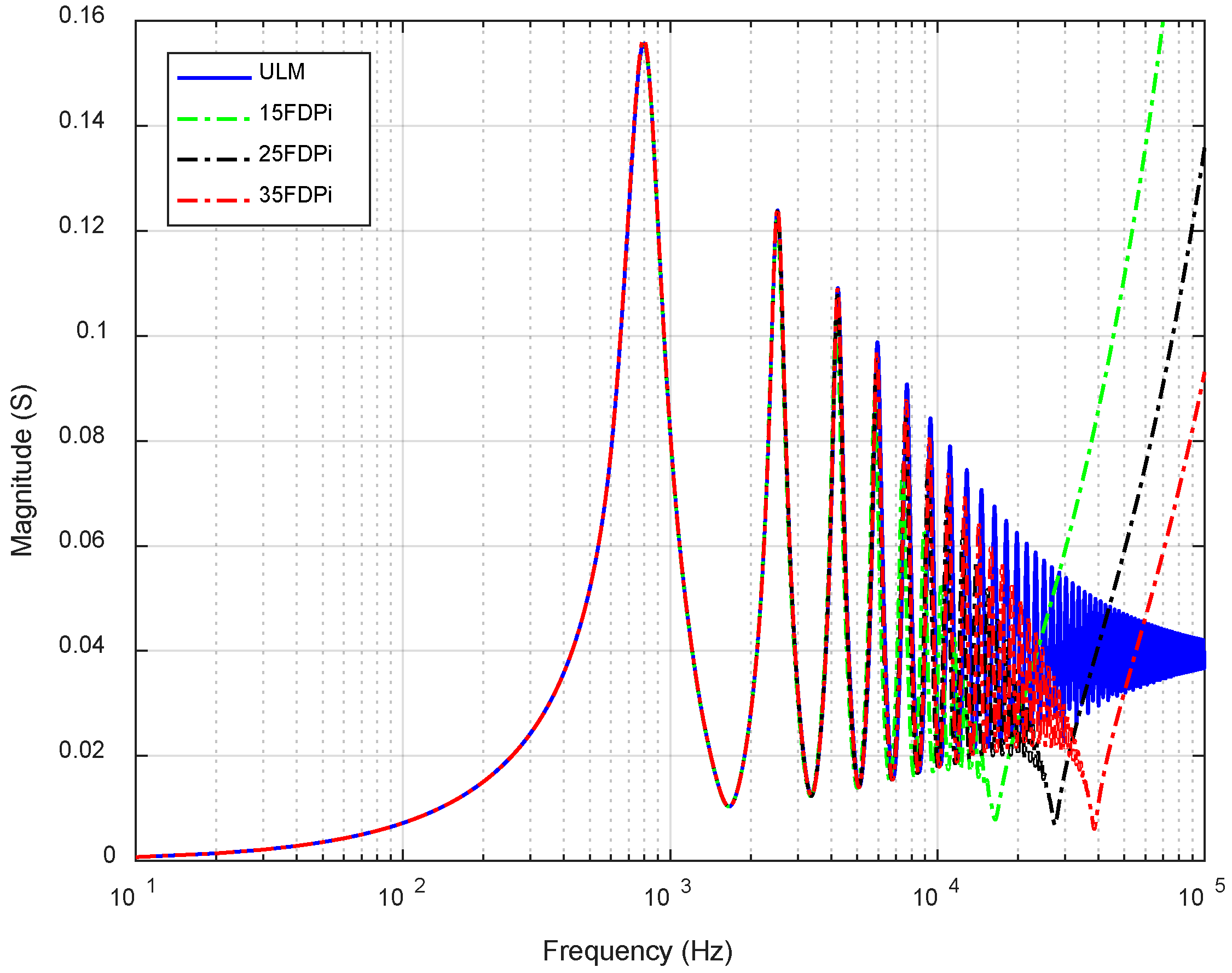
As presented in the previous case study, some changes are done to the number (N) of cascaded FDPi sections in order to show its effects on the frequency range and unreal resonance of the cable (Figure 14). Similar conclusions are obtained as in the previous example.
Figure 14.
Cable admittance comparison for Case Study #2 with different number (N) of cascaded FDPi sections.
As last point, it is worth to emphasize that all the parameters information for this cable is taken from reference [31]. In this reference, field measurements were done to a single section of a 150 kV underground cable and the results were compared with the Universal Line Model (ULM) from PSCAD/EMTDC software. The conclusions obtained in reference [31] describes a good agreement between measurements and ULM model for the coaxial mode of the real cable. In this sense, it can be stated that the results presented in this example indirectly validate the response of the FDPi model with experimental measurements.
5. Methodology for the Selection of the FDPi Model Order
As it can be inferred from the results shown in the previous section, the choice of an optimal model order, selection of M and N, does not obey deterministic rules and is highly dependent on several factors. This characteristic difficult the possibility of presenting guidelines that are valid for all the scenarios.
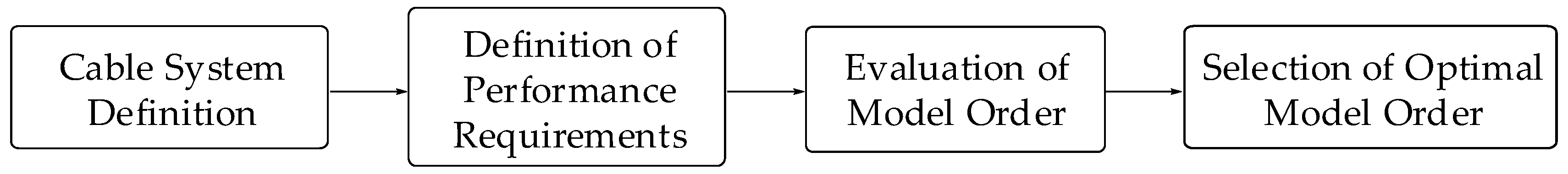
This section is intended to serve as a basis for creating a software tool that is capable of selecting a suitable model order for representing a given cable under specific performance requirements. Figure 15 shows the general procedure that should be implemented in the software tool for the determination of the optimal order of the FDPi model.
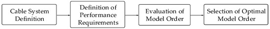
Figure 15.
General procedure for the determination of the optimal order of the FDPi model.
The first point to take into account is the definition of the cable system under study. This definition comes from the characteristics of the cable system, which are described next:
- Type of cable: Underground or submarine cables. Single-core or three-core cables.
- Cable length.
- Cable disposition: Tight or spaced disposition in flat or trefoil formation.
- Surrounding medium properties: resistivity and relative permeability of the surrounding medium.
- Burial depth.
- Grounding configuration: Single-end bonding, both-ends bonding or cross bonding.
- Load connected to the cable system: The cable impedance depends on the termination of the cable. This impedance can vary continuously (infinite possibilities). Extreme cases can be considered for the cable system, short-circuited cable and open-ended cable.
- Couplings between other cable systems.
All these aspects change the time response and frequency response of the cable; hence need to be evaluated in order to select an optimal model order.
The second step consists of defining the performance requirements that the FDPi model must fulfill. The most relevant requirements are:
- Frequency range: The definition of the frequency range is crucial for the intended application of the model. An adequate value should be assigned in order to include all the relevant dynamics that can have an effect on the studies that are going to be performed.
- Accuracy: It is necessary to define a minimum accuracy limit and quantify the accuracy. In order to quantify the accuracy, a measure of the error associated with the FDPi model must be defined. Several criteria can be used for the quantification of the error such as averaged error, weighted error and absolute error. Additionally, the error can be computed in the time domain, frequency domain or taking into account both domains. The authors suggest assessing the accuracy of the FDPi model in the frequency domain by computing the absolute error point by point over the frequency range of interest. Absolute error is chosen over other methods mainly to avoid a high error in a single frequency (for example in a resonance frequency). Furthermore, the accuracy of the FDPi model should be performed by evaluating the amplitude error and phase error separately. ULM can be considered as the reference model if measurements are not available.
The third block of Figure 15 consists of evaluating the order of the FDPi model. A sweep of M and N values should be performed for the cable system under study. Accuracy and computational time must be recorded for each M and N combination.
The last step is to select the optimal model. The selection of the optimal model order is a balanced trade-off between the following two conditions:
- Accuracy level within the allowable limit.
- The lowest computational time.
In general, higher values of M and N will lead to a better accuracy. However, beyond a certain model order, the improvements in accuracy with further increase of the model order tend to become almost negligible.
Another important aspect to take into account for the accuracy of the FDPi model is the way VF algorithm performs the approximation of the frequency-dependent variation of the electrical parameters of the cable system. Vector fitting algorithm may be fine-tuned by applying a weighting function [25]. This weighting function can improve the accuracy in a specific frequency region.
6. Potential Applications of the FDPi Model
The model presented in this paper is intended to be used in any computer-based simulation tool (such as Matlab/Simulink) with the aim of representing different cable-based scenarios. It can help in representing and analyzing the behavior of the cable for the steady state and for transient responses in both time domain and frequency domain. The main features of the model are:
- The capability of representing different types of cables (underground and submarine single core and three-core cables) and overhead lines.
- The capability of representing different cable dispositions or laying formations (flat formation, trefoil formation).
- The capability of representing different grounding configurations due to the fact of including the different conductive layers of the cable. In this sense, grounding configurations such as single end bonding, both ends bonding and cross bonding can be represented with the model.
- The possibility to derive simplified analytical models with different levels of abstraction from the complete model. This means that the model can be easily reconfigured with the aim of obtaining a model with a higher abstraction level that allows deducing dominant behaviors and parameters of the system under study, allowing to do many other subsequent analysis. All by obtaining a reduced computational cost model with reduced accuracy for higher frequencies.
- The possibility to configure a very accurate model at expense of the computational cost in order to study a specific or special phenomenon.
These previous features allow the correct characterization of the cable system: resonance frequencies, impedance spectrum, sequence impedances and impedance-admittance matrices.
As already presented in this paper, the FDPi model allows the formulation of a mathematical description, Laplace domain or state-space form, of the behavior of the cable. This feature allows the inclusion of the cable model with the mathematical description of other power components (such as transformers, filters, power converters including their control loops and harmonics, and others). Thus allowing the creation of a global analytical model of scenarios such as onshore and offshore wind power plants [32,33], electrically propelled vessels [34,35], electric railways, electrical grids [36] and many more, in where different types of cables and elements are presented. With this modeling approach, different valuable studies can be performed in order to obtain a higher understanding degree and contributing to the analysis and results presented in the previous references, which consider cable models at power frequency and neglecting their frequency dependent behavior.
Focussing the attention on an OWPP scenario, some of the valuable studies (in which the FDPi model can be used and contribute to them) can be oriented towards aspects in terms of system stability and power quality, as main industry concerns.
- System Stability:
- The development of a more complete analytical model of an OWPP scenario is required in order to perform this kind of study.
- The application of techniques (Nyquist and/or Lyapunov techniques) in order to analyze and evaluate the stability of the system.
- The design of solutions oriented towards the improvement of the stability of the system (design of controls and active damping strategies).
- Power Quality:
- The design of passive and/or active filters in order to damp the resonances presented in the OWPP.
- The improvement of the total harmonic distortion (THD).
- The evaluation of harmonics (harmonic assessment) based on the OWPP topology [37]. Possibility of this cable model to be used with the wind turbine harmonic model proposed in [11] and be able to test different modulation strategies, evaluate the fulfillment of BDEW [38] and IEEE 519 [39] grid codes, evaluate the propagation (magnitude and phase angle) of harmonics in the point of common coupling (PCC) and other points of the OWPP, and other studies.
This cable model can be used as well in the early design stages of the OWPP in order to contribute to the fulfillment of the design requirements. Some of these requirements can be the topology of the OWPP, the magnitude and frequency of the resonances, the maximum number of installable wind turbines (based on the topology), the fulfillment of low-voltage ride through (LVRT) and high-voltage ride through (HVRT) capability and many more.
7. Conclusions
In this paper, a frequency-dependent Pi model has been developed in order to reproduce the behavior of a three-core submarine cable.
The model consists of N cascaded FDPi sections. Each FDPi section incorporates the following: (i) the magnetic coupling which is represented by an inductance matrix, (ii) the electrical coupling between conductors and represented by means of capacitances, (iii) the frequency dependent variation of the conductive layers by means of Foster equivalent networks and iv) the loss mechanism of the cable represented with each resistive element. All these four points allow an easy implementation of the model by means of discrete RLC components.
Parameterization of the model is described in detail and is performed according to analytical equations. However, other parameterization methods can be used to account for proximity effect and other medium characteristics.
Regarding the validation of the FDPi model, two cable system case studies are presented and a comparison is performed with a reference model, the ULM model from PSCAD/EMTDC software. The first case presents the results of the FDPi model for the cable under study, a three-core submarine cable. The second case study presents the results of three single-core underground cables laid in trefoil formation. This last case confirms two important points in order to give more weight to the validity of the FDPi model. The first point is the model applicability to other types of cable systems and the second point is an indirect validation with experimental measurements that were performed on a real cable system for the coaxial mode.
The results for both case studies show a very good agreement of the FDPi model in representing the behavior of a power cable, submarine and underground cable, for frequencies up to 10 kHz. If a higher frequency range needs to be represented, the order of the model has to be increased in order to fulfill the accuracy requirements but at the expense of increasing the computational burden. Additionally, the effects of model order on the time response and the unreal resonance of the cable model are presented for a different number of cascaded FDPi sections.
Finally, it is important to emphasize that the choice of a suitable FDPi model order does not obey deterministic rules. It is highly dependent on the requirements such as desired accuracy and frequency range of interest on the one hand, and characteristics of the cable under study such as type of cable, cable configuration and cable length on the other hand.
Author Contributions
C.R.: conceptualization, formal analysis, investigation, software, writing—original draft preparation. G.A.: conceptualization, formal analysis, investigation, writing—review and editing. M.Z.: conceptualization, formal analysis, investigation, writing—review and editing. D.M.: conceptualization, formal analysis, investigation, writing—review and editing. J.A.: conceptualization, formal analysis, investigation.
Funding
This research received no external funding.
Conflicts of Interest
The authors declare no conflict of interest.
References
- Pineda, I. Offshore Wind in Europe—Key Trends and Statistics 2017; WindEurope: Brussels, Belgium, 2017. [Google Scholar]
- Watson, N.; Arrillaga, J. Power Systems Electromagnetic Transients Simulation; IET: Stevenage, UK, 2003; Volume 39, ISBN 9780852961063. [Google Scholar]
- Zhang, S.; Jiang, S.; Lu, X.; Ge, B.; Peng, F.Z. Resonance issues and damping techniques for grid-connected inverters with long transmission cable. IEEE Trans. Power Electron. 2014, 29, 110–120. [Google Scholar] [CrossRef]
- D’Arco, S.; Beerten, J.; Suul, J.A. Cable Model Order Reduction for HVDC Systems Interoperability Analysis. In Proceedings of the 11th IET International Conference on AC and DC Power Transmission, Birmingham, UK, 10–12 February 2015; p. 10. [Google Scholar]
- Pierre, R. Dynamic Modeling and Control of Multi-Terminal HVDC Grids. Ph.D. Thesis, Ecole Centrale de Lille, Villeneuve-d’Ascq, France, 2014. [Google Scholar]
- Hoshmeh, A. A Three-Phase Cable Model Based on Lumped Parameters for Transient Calculations in the Time Domain. In Proceedings of the IEEE Innovative Smart Grid Technologies, Melbourne, Australia, 28 November–1 December 2016; p. 6. [Google Scholar]
- Hoshmeh, A.; Schmidt, U. A full frequency-dependent cable model for the calculation of fast transients. Energies 2017, 10, 1158. [Google Scholar] [CrossRef]
- Meredith, R. EMTP Modeling of Electromagnetic Transients in Multi-Mode Coaxial Cables by Finite Sections. IEEE Trans. Power Deliv. 1997, 12, 489–496. [Google Scholar]
- Sakis, A.P.; Masson, J.-F. Modeling and Analysis of URD Cable Systems. IEEE Trans. Power Deliv. 1990, 5, 806–815. [Google Scholar]
- Macias, J.A.R.; Exposito, A.G.; Soler, A.B. A Comparison of Techniques for State-Space Transient Analysis of Transmission Lines. IEEE Trans. Power Deliv. 2005, 20, 894–903. [Google Scholar] [CrossRef]
- Ruiz, C.; Zubiaga, M.; Abad, G.; Madariaga, D.; Arza, J. Validation of a Wind Turbine Harmonic Model based on the Generic Type 4 Wind Turbine Standard. In Proceedings of the 20th European Conference on Power Electronics and Applications (EPE 2018), Riga, Latvia, 17–21 September 2018; p. 10. [Google Scholar]
- Lorenzo, E.D. The Maxwell Capacitance Matrix; FastFieldSolvers: Vimercate, Italy, 2011; pp. 1–3. [Google Scholar]
- Ametani, A. A general formulation of impedance and admittance of cables. IEEE Trans. Power Appar. Syst. 1980, PAS-99, 902–910. [Google Scholar] [CrossRef]
- Asada, T.; Baba, Y.; Member, S.; Nagaoka, N.; Ametani, A.; Fellow, L.; Mahseredjian, J.; Yamamoto, K. A Study on Basic Characteristics of the Proximity Effect on Conductors. IEEE Trans. Power Deliv. 2017, 32, 1790–1799. [Google Scholar] [CrossRef]
- Tsiamitros, D.A.; Papagiannis, G.K.; Dokopoulos, P.S. Earth return impedances of conductor arrangements in multilayer soils—Part II: Numerical results. IEEE Trans. Power Deliv. 2008, 23, 2401–2408. [Google Scholar] [CrossRef]
- Gustavsen, B.; Bruaset, A.; Bremnes, J.J.; Hassel, A. A finite-element approach for calculating electrical parameters of umbilical cables. IEEE Trans. Power Deliv. 2009, 24, 2375–2384. [Google Scholar] [CrossRef]
- Yin, Y.; Dommel, H.W. Calculation of frequency-dependent impedances of underground power cables with finite element method. IEEE Trans. Magn. 1989, 25, 3025–3027. [Google Scholar] [CrossRef]
- Pagnetti, A.; Xemard, A.; Paladian, F.; Nucci, C.A. An improved method for the calculation of the internal impedances of solid and hollow conductors with the inclusion of proximity effect. IEEE Trans. Power Deliv. 2012, 27, 2063–2072. [Google Scholar] [CrossRef]
- De Arizon, P.; Dommel, H.W. Computation of Cable Impedances Based on Subdivision of Conductors. IEEE Trans. Power Deliv. 1987, PER-7. [Google Scholar] [CrossRef]
- Patel, U.R.; Gustavsen, B.; Triverio, P. An equivalent surface current approach for the computation of the series impedance of power cables with inclusion of skin and proximity effects. IEEE Trans. Power Deliv. 2013, 28, 2474–2482. [Google Scholar] [CrossRef]
- Patel, U.R.; Triverio, P. MoM-SO: A Complete Method for Computing the Impedance of Cable Systems Including Skin, Proximity, and Ground Return Effects. IEEE Trans. Power Deliv. 2015, 30, 2110–2118. [Google Scholar] [CrossRef]
- Patel, U.R.; Triverio, P. Accurate Impedance Calculation for Underground and Submarine Power Cables Using MoM-SO and a Multilayer Ground Model. IEEE Trans. Power Deliv. 2016, 31, 1233–1241. [Google Scholar] [CrossRef]
- Gustavsen, B. Panel session on data for modeling system transients insulated cables. In Proceedings of the 2001 IEEE Power Engineering Society Winter Meeting (Cat. No. 01CH37194), Columbus, OH, USA, 28 January–1 February 2001; Volume 2, pp. 718–723. [Google Scholar] [CrossRef]
- Da Silva, F.M.F. Analysis and Simulation of Electromagnetic Transients in HVAC Cable Transmission Grids. Ph.D. Thesis, Aalborg University, Aalborg, Denmark, 2011. [Google Scholar]
- Gustavsen, B.; Semlyen, A. Rational Approximation of Frequency Domain Responses by Vector Fitting. IEEE Trans. Power Deliv. 1999, 14, 1052–1061. [Google Scholar]
- Gustavsen, B. Improving the pole relocating properties of vector fitting. IEEE Trans. Power Deliv. 2006, 21, 1587–1592. [Google Scholar] [CrossRef]
- Deschrijver, D.; Mrozowski, M.; Dhaene, T.; De Zutter, D. Macromodeling of multiport systems using a fast implementation of the vector fitting method. IEEE Microw. Wirel. Compon. Lett. 2008, 18, 383–385. [Google Scholar] [CrossRef]
- XLPE Submarine Cable Systems; Asea Brown Boveri: Zurich, Switzerland, 2014.
- Gustavsen, B.; Martinez, J.A.; Durbak, D. Parameter determination for modeling system transients—Part II: Insulated cables. IEEE Trans. Power Deliv. 2005, 20, 2045–2050. [Google Scholar] [CrossRef]
- Zubiaga, M.; Abad, G.; Barrena, J.A. Energy Transmission and Grid Integration of AC Offshore Wind Farms; Intech: London, UK, 2012; ISBN 978-953-51-0368-4. [Google Scholar]
- Gudmundsdottir, U.S. Modelling of long High Voltage AC Cables in the Transmission System. Ph.D. Thesis, Aalborg University, Aalborg, Denmark, 2010. [Google Scholar]
- Hou, P.; Ebrahimzadeh, E.; Wang, X.; Blaabjerg, F.; Fang, J.; Wang, Y. Harmonic Stability Analysis of Offshore Wind Farm with Component Connection Method. In Proceedings of the 43rd Annual Conference of the IEEE Industrial Electronics Society (IECON 2017), Beijing, China, 29 October–1 November 2017. [Google Scholar]
- Jing, L.; Son, D.-H.; Kang, S.-H.; Nam, S.-R. Unsynchronized Phasor-Based Protection Method for Single Line-to-Ground Faults in an Ungrounded Offshore Wind Farm with Fully-Rated Converters-Based Wind Turbines. Energies 2017, 10, 526. [Google Scholar] [CrossRef]
- Alacano, A.; Valera, J.J.; Abad, G.; Izurza, P. Power Electronics Based DC Distribution Systems for Electrically Propelled Vessels: A Multivariable Modeling Approach for Design and Analysis. IEEE J. Emerg. Sel. Top. Power Electron. 2017, 6777, 19. [Google Scholar] [CrossRef]
- Alacano, A.; Valera, J.J.; Abad, G. A Multivariable Modeling Approach for the Design of Power Electronics Based DC Distribution Systems in Diesel-Electric Vessels. In Proceedings of the IEEE 17th Workshop on Control and Modeling for Power Electronics (COMPEL), Trondheim, Norway, 27–30 June 2016. [Google Scholar]
- Abad, G.; Laka, A.; Saavedra, G.; Barrena, J.A. Analytical modeling approach to study harmonic mitigation in AC grids with active impedance at selective frequencies. Energies 2018, 11. [Google Scholar] [CrossRef]
- Liu, Z.; Rong, J.; Zhao, G.; Luo, Y. Harmonic Assessment for Wind Parks Based on Sensitivity Analysis. IEEE Trans. Sustain. Energy 2017, 8, 1373–1382. [Google Scholar] [CrossRef]
- Bartels, W.; Ehlers, F.; Heidenreich, K.; Huttner, R.; Kuhn, H.; Meyer, T.; Kumm, T.; Salzmann, J.M.; Schafer, H.D.; Weck, K.H. Generating Plants Connected to the Medium-Voltage Network; BDEW Technical Guideline: Berlin, Germany, 2008. [Google Scholar]
- IEEE Working Group PQ-Harmonics. IEEE Std 519-2014—IEEE Recommended Practice and Requirements for Harmonic Control in Electric Power Systems; IEEE: New York, NY, USA, 2014. [Google Scholar]


© 2018 by the authors. Licensee MDPI, Basel, Switzerland. This article is an open access article distributed under the terms and conditions of the Creative Commons Attribution (CC BY) license (http://creativecommons.org/licenses/by/4.0/).