A New Optimal Selection Method with Seasonal Flow and Irrigation Variability for Hydro Turbine Type and Size


Industrial and Manufacturing Engineering Department, School of Engineering of Technology, Asian Institute of Technology, Pathumthani 12120, Thailand
*
Author to whom correspondence should be addressed.
Energies 2018, 11(11), 3212; https://doi.org/10.3390/en11113212
Submission received: 19 October 2018
/
Revised: 16 November 2018
/
Accepted: 16 November 2018
/
Published: 20 November 2018
(This article belongs to the Special Issue Sustainable Energy Development Strategies: Energy Efficiency and Renewables)
Abstract
:A micro hydropower plant of the run-of-river type is considered to be the most cost-effective investment in developing counties. This paper presents a novel methodology to improve flow estimation, without using the flow direction curve (FDC) method, to determine the turbine type and size to operate consistently. A higher precision is obtained through the use of seasonal flow occurrence data, irrigation variability, and fitting the best probability distribution function (PDF) using flow data. Flow data are grouped in classes based on the flow rate range. This method will need a larger dataset but it is reduced to a tractable amount by using the PDF. In the first part of the algorithm, the average flow of each range is used to select the turbine type. The second part of the algorithm determines the optimal size of the turbine type in a more accurate way, based on minimum and maximum flow rates in each class range instead of the average flow rate. A newly developed micro hydropower plant was installed and used for validation at Baan Khun Pae, Chiang Mai Province. It was found, over four years of observation from 2014–2018, that the plant capacity factor was 82%.
1. Introduction
Global installed hydropower capacity has been growing in recent years by an average of 24.2 GW per year. The International Energy Agency has predicted the long-term deployment of hydropower. Installed hydropower capacity will increase to nearly twice the current level of 1947 GW by 2050 [1]. Hydropower plants can be classified based on the installed power generation capacity [2]. When the installed capacity of a hydropower plant is below 10 MW, it is called a small hydropower plant; when the capacity is up to 100 kW, it is called a micro hydropower plant; and when the capacity is below 10 kW, it is called a mini or pico hydropower plant. Micro and pico hydropower plants are usually in the form of run-of-river schemes [3]. Run-of-river hydropower plants are useful in remote areas where there is a need for energy for human development. At the same time, these plants can create sustainable energy with minimal impact to the surrounding area and communities. Electrical production of run-of-river hydropower plants depends on the locally available water resources. In general, the purpose of a hydropower system is to convert the potential energy of the river into mechanical energy in a turbine shaft, which is connected with an electric generator. The output of a hydropower plant is given in terms of power (kW) and electricity production (kWh). The power input is a function of water flow and net head. These variables are needed for evaluating the installed capacity and determining the appropriate turbine type and size.
Some researchers have presented the advantages of installing several small turbines instead of large ones. Using two or three smaller turbines allows easier control of water usage, although this requires more equipment and carries a higher operational cost [3,4]. Voros et al. [5] presented a short-cut design of small run-of-river hydroelectric plants. The minimum and maximum value of water flow was used in this approach for maximizing economic benefits of investment. Montanri [6] studied the economic compatibility of hydropower plants by regularizing the duration curve and the turbine efficiency. Hosseini et al. [7] determined the optimal installation capacity of existing run-of-river small hydropower plants (SHPs) depending on the amount of annual energy, economy, and reliability. The water flow from the flow duration curve (FDC) was used to calculate the annual energy generated. Anagnostopoulos and Papantonis [8] studied the optimal installation capacity of a run-of-river type SHP to assess the economic benefits of the investment. They optimized two parallel turbines of different types and sizes and found the net present value based on annual energy production. The water flow used in different operating ranges of the turbine is the key to more efficient operation. Santolin [9] presented a techno-economical method for predicting the installed capacity of SHPs. A model was developed on the basis of the flow availability of the site, represented by the FDC. The influence of the design operating conditions based on the FDC was used to determine the turbine size and investment cost. Monterio et al. [10] presented a novel short-term forecasting model of electric power production of existing SHPs. The available water flow was used to determine the power production, economy, and maintenance scheduling of the plants. Bortoni et al. [11] presented a novel methodology for the optimal online operation of hydropower plants provided with a single penstock. This method used the flow rate and head value under several conditions for the optimal distribution of the dispatched power amount. Additionally, Paish [12] presented plans for the future development of run-of-river hydropower plants. Future developments are toward the more accurate and rational sizing of systems to maximize their financial return.
Most researchers have focused their attention on the optimal installed capacity and the optimal turbine operation of existing hydropower plants based on the turbine operation flow rate range or the potential energy evaluation from the available water resource, as shown in Table 1. They chose the design flow value from the proportion of time a certain streamflow is exceeded which is approximately between 90 to 95% of streamflow occurrence throughout the year from the FDC. Subsequently, the type and size of commercial hydro turbines were considered to optimize the energy production. The results can yield more than one type of turbine for the same operational condition. In general, designs of commercial hydro turbines are standardized, and are not customized for local water resources that are available for all seasons. These commercial turbines are not always operated consistently at the highest efficiency because the design of the turbines is usually determined by the manufacturers. This seems to guarantee that the turbine will operate nearly continuously. However, in reality the operation time is much less than 70%. This could be due to inaccurate FDCs or wrong type and size selection.
According to the Energy Policy and Planning Office, Thailand Ministry of Energy, Thailand has set a target to increase its number of SHPs in 2021 by 20% from the current level. Water resources in many areas of Thailand have been surveyed for the installation of SHPs [13,14]. Additionally, the Provincial Electricity Authority (PEA) has installed run-of-river SHPs in several remote communities in Northern Thailand [15]. There are problems with the hydro turbine currently used by the PEA, as it cannot be operated continuously. The turbine can only work well during the rainy season, which lasts approximately five to six months. In dry seasons, the water flow into the system is quite low and not sufficient to operate the turbine. Average data collected over 25 years for six run-of-river SHPs of the PEA are shown in Table 2, and confirm the problem that the average electrical power production value of each hydropower plant is quite different from the installed capacity. This is because the available streamflow value at each site was overestimated from the FDC in order to achieve a high installation capacity in the wet season. However, there is a problem in the dry season. Additionally, the ratio of average electrical power production to installed capacity for each hydropower plant capacity factor is less than 50%, which confirms the above problems and includes the effect of the economic returns from the project.
This paper presents a new way to obtain a more precise flow rate estimation without using the FDC method to determine the optimal turbine type and size, to allow consistent turbine operation throughout the year. This higher precision is obtained using the seasonal flow occurrence data, irrigation variability, and fitting a probability distribution function (PDF) using the observed flow data. This approach provides a more precise estimation than the FDC method. Additionally, for the turbine size selection, the use of the minimum and maximum flow rate of operation is used to optimize the operation time. The final results of this algorithm are optimal turbine type and size based on the maximum annual energy production. This case study uses actual streamflow data from the Baan Khun Pae River, Chom Thong District, Chiang Mai Province, Thailand, including information from the Baan Khun Pae micro hydropower plant.
2. Potential Energy Estimation
2.1. Historical Flow Data
Historical flow data were obtained from the main river gauge station data at the Royal Irrigation Department (RID) in Thailand. Historical streamflow data were used to consider streamflow trends and variability. Data for the closest gauge station to the study site, located at the Num Mae Cheam River, were available from 1953 to 2007. The catchment area of this gauge station covered the Baan Khun Pae (BKP) River; the distance between the gauge station and the BKP River is approximately 12 km. The tendency of streamflow occurrence for the streamflow data recorded at this gauge station did not have an exact pattern. The variance of historical streamflow data can be expressed by the standard deviation (SD). The SD of streamflow data set in each month are shown in Figure 1. A low SD in March shows that the streamflow data points tended to be very close to the mean or monthly average value. The variance of streamflow occurrence in this month is small, which is more accurate for prediction. On the other hand, the high SD in September shows that the streamflow values are spread out over a large range. Therefore, the prediction of the streamflow occurrence in this month will be less accurate.
In order to predict streamflow occurrence in the study area, the variability of monthly streamflow for various years was plotted, as shown in Figure 2. The middle line presents the mean of all values in the streamflow data set, the upper line indicates the mean value plus the standard deviation, and the bottom line shows the mean value minus standard deviation; the area of both graphs is the area between the top and bottom line, and is called the probability area. This area can be used to predict the streamflow occurrence. Some data points are outside the probability area, however, most of the data points are within it. This means that in every year, the streamflow can be greater or less than the monthly average streamflow (middle line), but will not exceed the mean value plus or minus the standard deviation.
2.2. Observed Flow Data
After determining the trend of streamflow occurrence in this area, the actual available streamflow in Baan Khun Pae River is measured to estimate the potential energy production and plant capacity. Several techniques for measuring the flow in streams can be separated into two main classes of techniques: direct and indirect measurement methods [17,18]. Direct measurement methods consist of several methods, such as the velocity area method, moving boat current method, dilution method, electromagnetic method, and ultrasonic method. Direct measurement methods are conventionally used for medium to large rivers. Not all of these methods are generally applicable: each will be used in the respective power plant depending on different aspects including compatibility, economy, and accuracy. There are two indirect measurement methods: the weir method and slope area method.
In this study, the weir method is used to calculate water flow of the Baan Khun Pae River because it has a small concrete weir to store water. Some studies have recommended this method for measuring the flow of small rivers [19,20,21]. Furthermore, the weir method is the most accurate and reliable flow measurement method; the accuracy should be about ±1.7 to ±3% and the flow condition should not be more than 4 m3/s [21]. The principle of the weir method is to measure the free surface flow and to observe the head over the weir. Frequency of observation is important because the accuracy and reliability of flow estimates depend on this value. Therefore, in order to check the precision of the flow measurement, the water level over the concrete weir should be measured twice a day every day throughout the year. Results are shown in Figure 3.
2.3. Annual Irrigation Demand Estimation
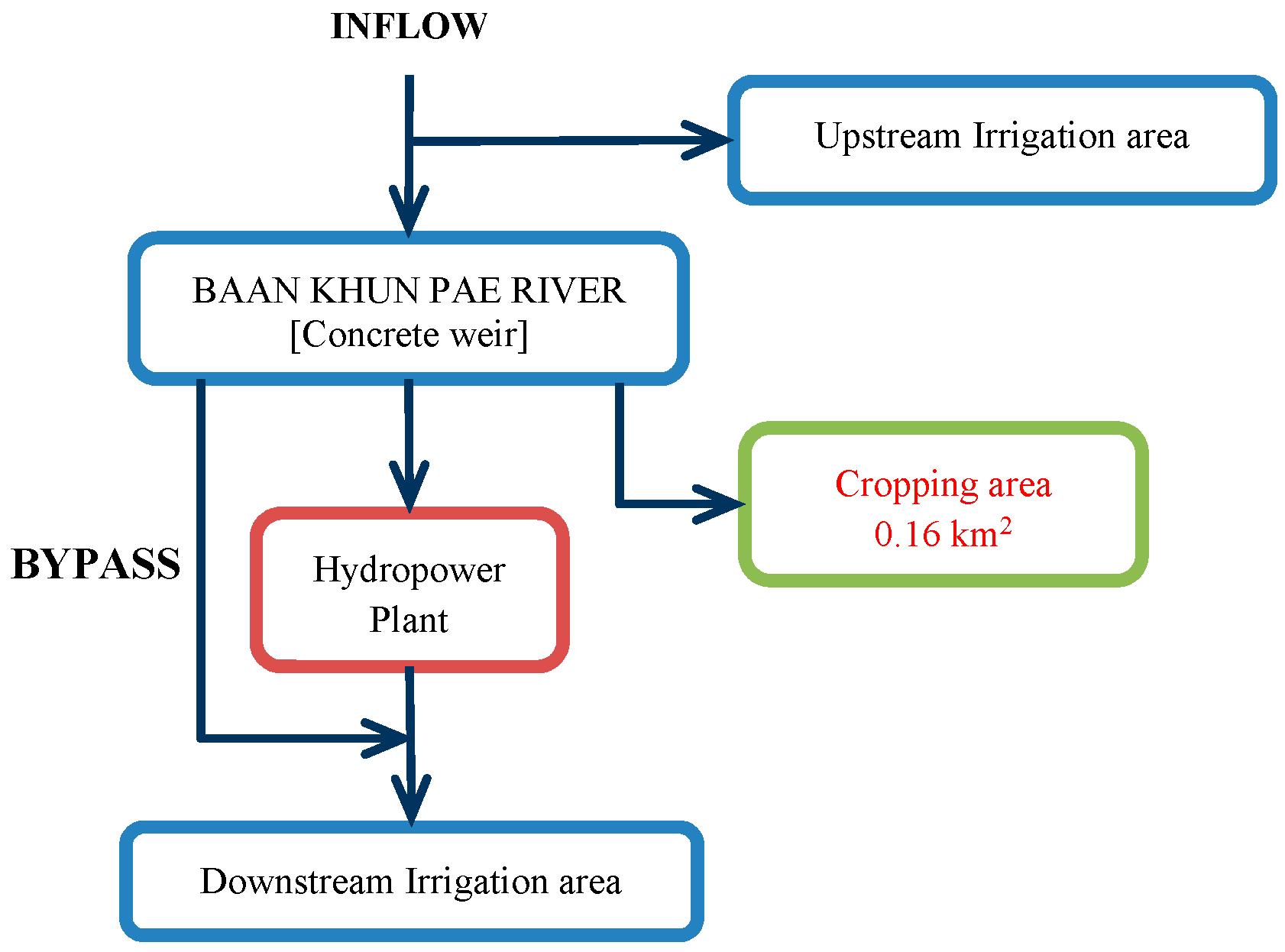
The upstream and downstream irrigation areas are approximately 56 km2, including the community area of 1.1 km2, the agricultural area of 19 km2 and the forest conservation area of 35.9 km2. This is the total area used in both the wet and dry seasons. The dry season is from December to June and the wet season is from July to November. Rice is the main wet-season crop, accounting for 70% of the area, while perennial and vegetable crops account for 30%. Dry season cropping will consist of 45% vegetables, 20% herbs, 15% ornamental and other upland crops, and 25% perennials. The schematic simplified irrigation demand of the Baan Khun Pae area is shown in Figure 4. The upstream irrigation areas use the inflow water from the mountain for crop growing and irrigation demand. The remaining water flows to the concrete weir of the hydropower plant. The downstream irrigation areas use the water from the tail race of the hydropower plant and the water over the concrete weir (bypass) for cropping and irrigation demand. There is also a cropping area of 0.16 km2 that receives water from the concrete weir for vegetable cropping. Thus, the water flow at the concrete weir is divided into three parts—bypass, hydropower plant, and cropping area. The water used by the cropping area throughout the two-year period depends on the climate and streamflow occurrence. The average monthly water flow requirement of the cropping area is shown in Figure 5. The observation data of the streamflow occurrence at the concrete weir and the average monthly water flow requirement of the cropping area are used to estimate the water flow available for the hydropower plant to produce electrical energy. Based on the water flow over the concrete weir (bypass), it is estimated that less than one percent of the remaining water flow is available to sustain aquatic life in the area. Therefore, the amount of remaining water at the concrete weir will be used to estimate the maximum annual energy production of the hydropower plant.
2.4. Estimation of the Available Streamflow
There is no available flow record and the measured streamflow for only one year is not accurate enough to evaluate the available energy. The measurement error and some missing flow data, when heavy rain occurred, affect the accuracy of the energy estimation. This problem can be solved by using a PDF. Various distribution functions have been used to increase the reliability of observation data, such as the Weibull distribution, lognormal distribution, and Gamma distribution. One of the distribution functions will be used to obtain the probability of the observed values. Many textbooks and researchers have recommended a good estimate of the distribution parameters by using the maximum likelihood method [22,23,24]. This study considers three different probability distributions which are widely used in hydrology distribution analysis.
The three different distributions are fitted to the observation values, and parameters of distributions are estimated using the maximum likelihood method. The “statistic toolbox” function in MATLAB is used for this purpose. Results are shown in Table 3. The estimated parameters of the distributions based on the maximum likelihood method show that the Gamma distribution performs better than the other distributions. Figure 6 shows a comparison between the fitted Gamma distribution and the frequency of the observation values from Figure 5. The observed flow rates were grouped into 20 classes with a range of 0.05 m3/s.
The scale (mean) and shape (variance) parameters of the Gamma distribution function were used to generate the streamflow data set based on the observed flow data in one year. The streamflow data set for each day within one year (365 samples) is used to estimate the potential energy production of the BKP micro hydropower plant. The comparison of observation data in one year and generated streamflow data set from the Gamma distribution function is shown in Table 4. The probability of the generated streamflow data set is represented by the histograms shown in Figure 7. Note that there is less variability of the data compared with Figure 6.
3. Turbine Type Selection
The selection of the turbine depends upon the site characteristics. The main characteristics that should be considered to select the turbine type are the head and flow available, the desired running speed of the generator, and whether the turbine will be expected to operate in variable flow conditions. Hydro turbines can be classified into two main groups based on the flow pattern in the turbine and the specific speed. Based on the flow pattern, hydro turbines are categorized into three groups: high, medium, and low head. These are grouped into two categories: impulse and reaction turbines. The difference between impulse and reaction turbines can be explained by water pressure. When the water pressure applies a force on the face of the runner blades, which decreases as it proceeds through the turbines, these are called reaction turbines. A reaction turbine needs a higher volume flow rate to operate than an impulse turbine. There are three main types of reaction turbine used: the propeller, Kaplan, and Francis turbines. For impulse turbines, all the water pressure is converted into kinetic energy before entering the runner. Kinetic energy is in the form of a high-speed jet that strikes the buckets, mounted on the periphery of the runner. There are three main types of impulse turbines used: the Pelton, Turgo, and cross-flow turbines. All variables are related to the turbine specific speed. The specific speed of turbine types is the most suitable parameter on which to base the selection of a turbine. In general, low turbine specific speed of an impulse turbine corresponds to low flow rates and high heads, whereas high turbine specific speed of a reaction turbine corresponds to high flow rates and low heads. The turbine specific speed is given by the dimensionless parameter [25]:
where NS is the turbine specific speed, NR is the angular velocity (rad/s), QD is a design flow (m3/s), and HN is an effective head (m). Commonly, the micro hydro turbine should be operated at the normal speed of a standard generator. Therefore, the specific speed equation is used in this algorithm for selecting turbine type by fixing the turbine shaft speed. The normal operating ranges for the turbine specific speed and the effective head for each turbine type are shown in Table 5.
4. Annual Energy Production Estimation
The energy potential of a run-of-river power plant is proportional to the flow and the head. Here, the operation range is used to estimate the annual energy production. The operation range of each turbine type is different. The turbine can operate when the water flow rate is between a minimum (Qmin) and a maximum (Qmax) value. Penche [3] presented the minimum technical flow for different types of turbines. The minimum flow for each turbine type is given as a percentage of design flow as shown in Table 6.
The design flow (QD) or water flow rate through the turbine is determined by the following relationship as a function of the available streamflow (Qav):
If the available streamflow is less than the minimum flow rate of the turbine, the turbine will shut down. On the other hand, if the available flow rate is more than the maximum flow rate of the turbine, the maximum flow rate or design flow will be used to operate the turbine because the intake gate and the difference of water level at the small weir of run-of-river will not affect the turbine performance. Therefore, the decision to select the design flow of each turbine type and size will be limited by Equation (2). In order to increase the reliability of micro hydro turbine operation and increase the accuracy of the potential energy estimation, the probability of streamflow occurrence is used to evaluate the maximum annual energy production, given by
where E is the maximum annual energy production (kWh/year), QD is the design flow (m3/s), HN is the effective head or net head (m), Pri is the probability of streamflow occurrence within the range, h is the number of operation hours within a year (h/year), i is the sequence of streamflow range, and n is the total number of streamflow ranges.
5. Optimal Turbine Type and Size Selection Algorithm
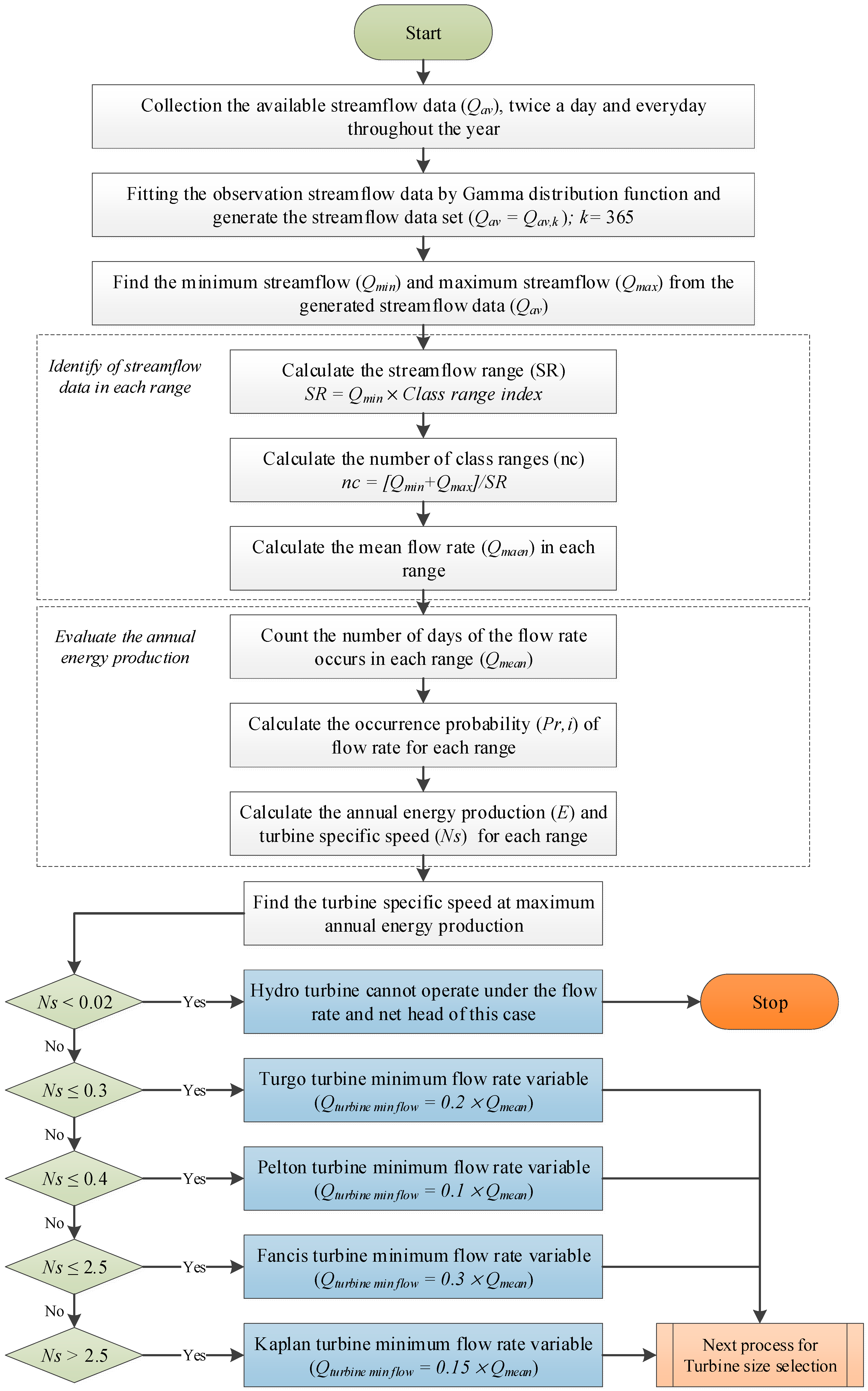
The selection algorithm is separated into two main processes. The first process is selecting the turbine type and minimum flow variable for the operation of each hydro turbine type, as shown in Figure 8. The results of the first process will be used for the second process, which is to find the optimal turbine size after type selection, as shown in Figure 9. The first two steps of the first process are the collection and analysis of observation flow data, including the irrigation demand. The Gamma distribution function is used to generate the streamflow data set for one year (365 samples). Thence, the streamflow data set are arranged from larger values to smaller values. The next steps in the flowchart are finding the maximum streamflow (Qmax) and minimum streamflow (Qmin) from the generated streamflow data (Qav) (365 samples). The class range index is used to select the streamflow range (SR) to calculate the number of class ranges (nc). In each class range (i) the mean streamflow (Qmean) is used to count the streamflow occurrence number of days to evaluate the probability of occurrence (Pr,i). Then, each streamflow range is associated with this probability to evaluate the annual energy production and turbine specific speed. The first iteration starts from the minimum flow rate value (Qmin), and it has a high probability of occurrence. This iteration process continues until the last class range (nc). After that, the turbine specific speed at maximum annual energy production (Equation (3)) is used to select the turbine type and minimum flow rate to operate. If the turbine specific speed value is lower than 0.02 the algorithm is stopped because the lowest streamflow and net head are not suitable; otherwise, it will recommend the best type. The type results in the first process are then used in the second process to select the size (Figure 9).
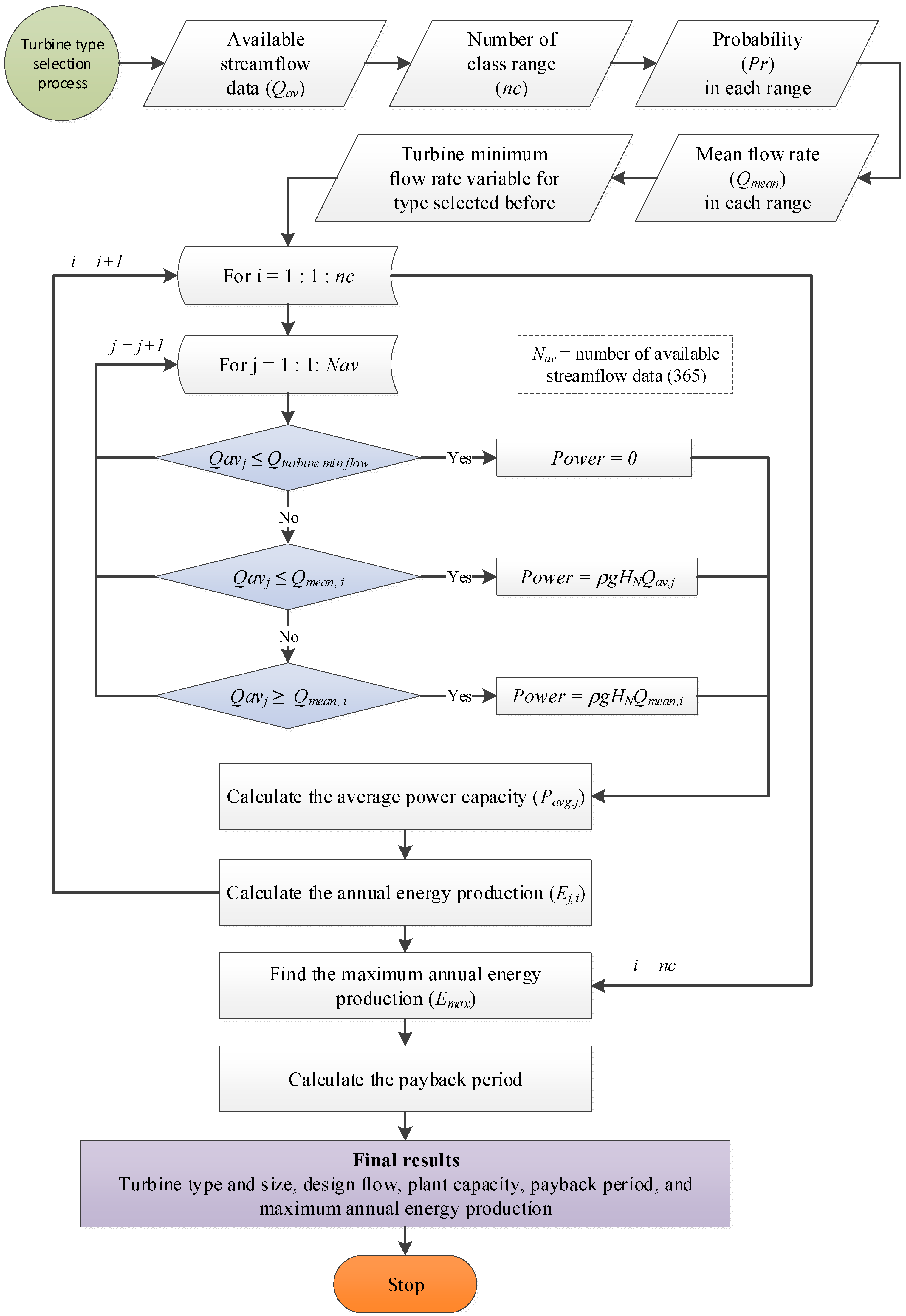
The second process finds the turbine size based on a more accurate way of calculating maximum potential energy production. The streamflow data (Qav), mean flow rate (Qmean), probability of streamflow occurrence (Pr,i), and number of class ranges (nc) are used. Especially, the minimum flow rate variable of the turbine type is used to check the operation condition of the turbine. The first iteration begins from the mean streamflow (Qmean) in the first-class range. The streamflow data between mean streamflow (Qmean) and turbine minimum streamflow (Qturbine min flow) are used to check the operation condition before computing the annual energy production. If the available streamflow is lower than the minimum streamflow, the turbine will be shut down and the energy is equal to zero.
On the other hand, if the available streamflow (Qav) is less than or equal to the mean streamflow (Qmean) of the turbine condition, the available streamflow is used to evaluate the power capacity. If the available streamflow (Qav) is more than the mean streamflow (Qmean) of the turbine condition, the mean streamflow is used to calculate the power capacity. This loop stops with the last sequence of streamflow data (j = 365). After that, the average power capacity (Pavg) in this range is used to compute the annual energy production (E). The mean streamflow is changed to the next class range until the last class range (i = nc) is reached. The maximum annual energy production is used to determine turbine size. The last process is to check the cost–benefit ratio of the proposed turbine type and size and calculate the design flow. Information about the maintenance costs of the hydro turbines under supervision of PEA, the average annual income from electricity sales of PEA, and the investment costs of turbines are used for this step. The final outputs of this algorithm are a turbine type and size, maximum annual energy production, design flow, plant capacity, and payback period. The design flow value is then used to design the detailed turbine geometry.
6. Results and Discussion
Based on the histogram of probability of streamflow occurrence from Figure 7, the streamflow range is 0.0175 m3/s for a total of 20 class ranges. Therefore, the first-class range of flow rate is 0.0001–0.0175 m3/s, which encompasses the flow rate values for 289 days. The mean flow rate of this range, 0.0088 m3/s, has a high probability of occurrence of approximately 80%. The power capacity, annual energy production, and turbine specific speed in this range are 6.73 kW, 39,015 kWh, and 0.0567, respectively. For the next class range, the flow rate range is greater than that of the first class, and will be used to calculate the next annual energy production until the last class range with the lowest probability of occurrence.
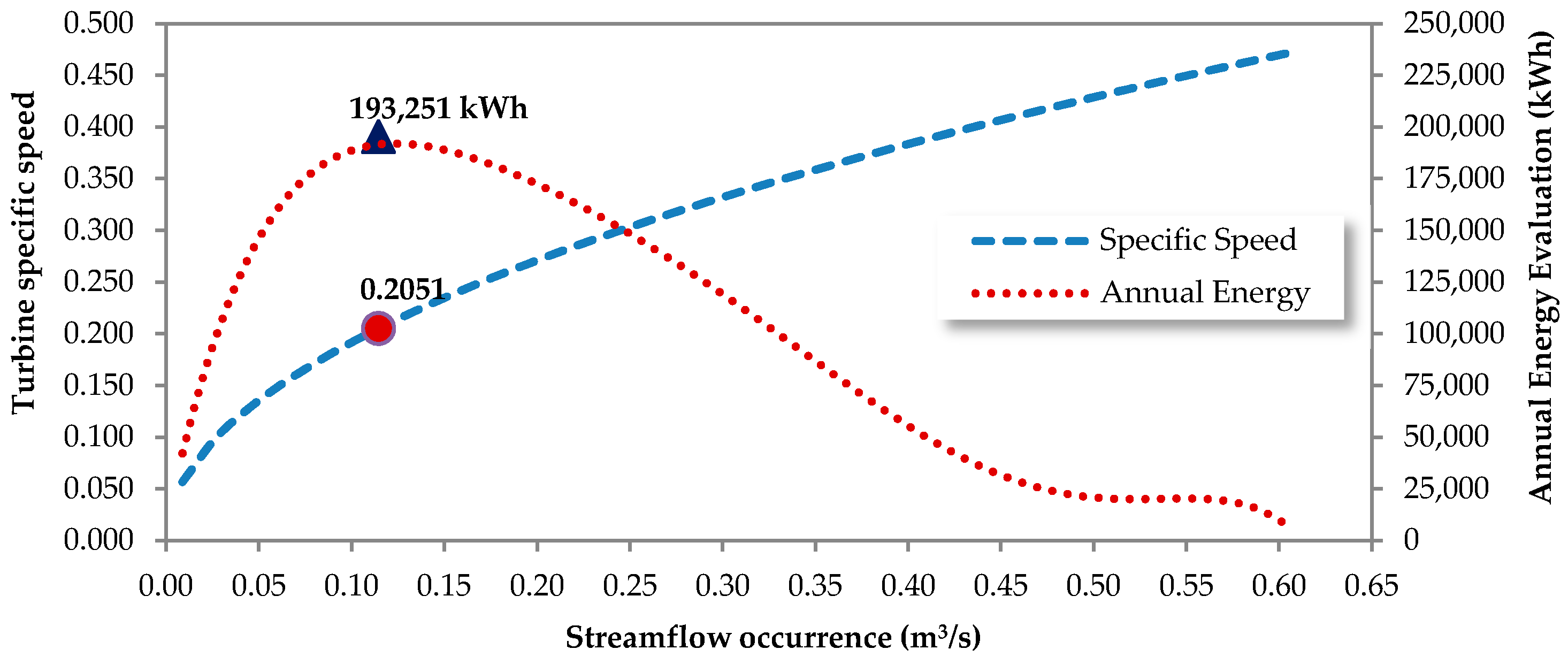
The class range index (see Figure 8) does change the flow range in each class. A higher value of class range index will result in a lower number of classes. The class range index was selected to be as small as possible so that further increases did not change the resulting maximum energy production in the turbine type selection algorithm. This was obtained with 200 classes for a class range index of 36 through trial and error. The comparison of annual energy production results and turbine specific speeds for 200 classes are shown in Figure 10. High flow rates have a lower probability of occurrence and produce low annual energy. On the other hand, low flow rates have a high probability of occurrence, and allow the turbines to produce larger amounts of annual energy. The impulse turbine is more popular in micro hydropower plant selection than the reaction turbine because it is cheaper and easier to maintain. Moreover, impulse turbines have lower frictional losses than reaction turbines, which affects the flow rate range to operate the turbine. From the results, the turbine specific speed is 0.2051 at maximum annual energy production, which is in the range of the Turgo and Pelton turbines. Both turbines are suitable in this case because of the low flow rate and high effective head. The Turgo turbine will have a smaller diameter than the Pelton turbine. Therefore, it can be concluded that the Turgo turbine is a better choice for this case study than the Pelton turbine.
As shown in Figure 8, the optimal turbine type selection algorithm uses the mean flow rate in each range to compute the estimation of power capacity and annual energy production. As shown in Figure 10, the optimal turbine size selection algorithm will use the Qmin cut of values to calculate the power of the turbine operation. Considering the maximum annual energy production (Figure 11), the probability of streamflow occurrence is approximately 30%, which can produce a power capacity of 87.95 kW.
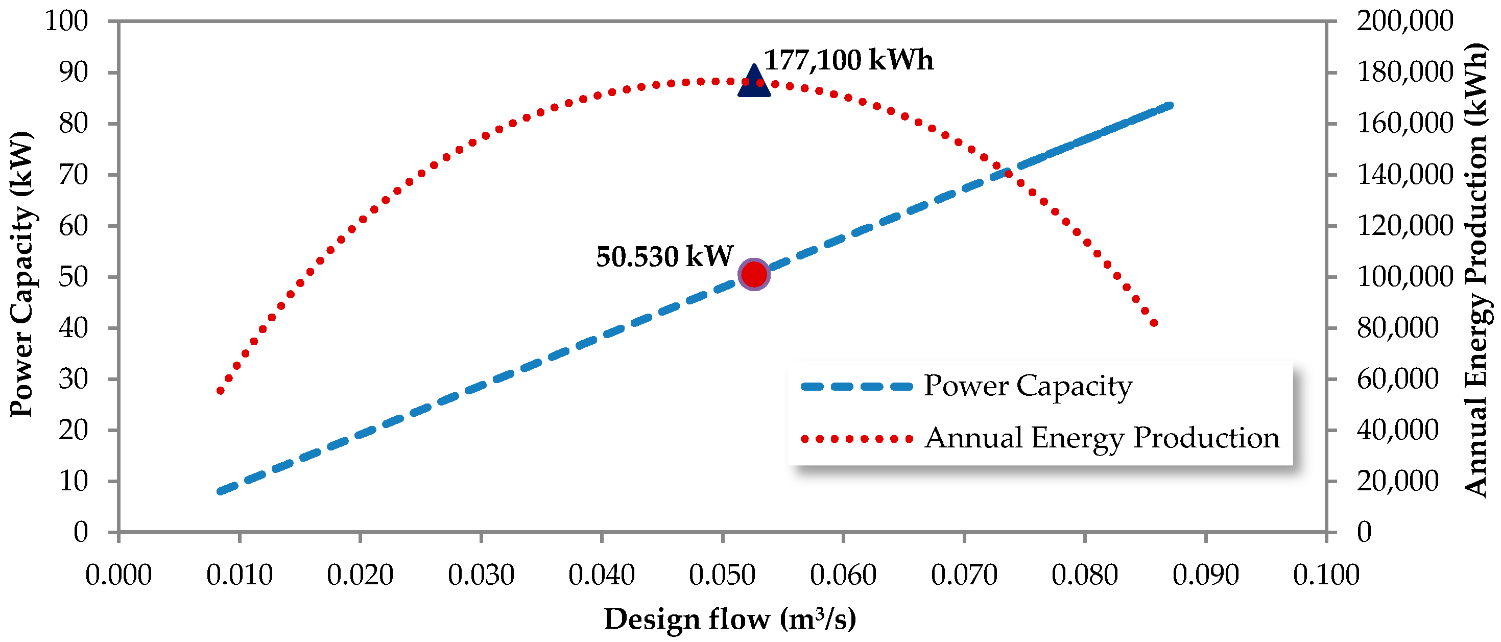
In order to increase the accuracy, the operation range of the Turgo turbine, as calculated using Equation (2), was used to estimate the annual energy production. The minimum flow rate for operating the hydro turbine (Table 6) and information regarding the maintenance costs of the Turgo turbines under supervision of the PEA are used in the optimal turbine size selection algorithm, as shown in Figure 9. The average annual income from electricity sales of the PEA is around 0.105 USD per kW. The investment cost determined in this study does not include civil work, only mechanical and electrical works of the Turgo turbine type, the cost of which is approximately 1250 USD per kW. The condition of turbine operation based on turbine minimum flow rate is very important to accurately estimate the precise turbine size, since if the available flow rate is lower than the minimum flow rate value the turbine will be shut down. In contrast, if the available flow rate is higher than the design flow value, the turbine will use the design flow rate value to produce electricity. The accuracy of this algorithm will depend on the amount of available streamflow data. If there is a large amount of data, the accuracy of the result will be higher. Furthermore, energy production depends on the operational turbine performance. The final results show that the Turgo turbine can produce a maximum annual energy of 0.1771 GWh with a payback period of 1197 days. The minimum flow rate required to operate is 0.0105 m3/s, with a design flow of 0.0526 m3/s at a net head of 98 m and a turbine shaft speed of 1000 rpm. The plant capacity is 50 kW. It is possible to compare the more accurate maximum energy estimate by comparing Figure 10 and Figure 11 with the results from the second phase of the algorithm (Figure 12).
7. Conclusions
A novel methodology for estimating the energy production of a hydro plant based on observation, irrigation demand, and historical flow data was developed and implemented. The results were used to determine optimal turbine type and size. Streamflow was measured and fitted with the best PDF. The flow data were grouped into classes based on flow rate range. Flow occurrence curves were used to compute the total annual energy production for various turbine parameters. An algorithm was developed to find the optimal turbine type and size based on the maximum annual energy production. In the first part of the algorithm the average flow of each range was used. The average flow of the class that gives the highest annual energy was used to select the turbine type. The number of classes used is important: the higher the number of classes, the more accurate the results. The class number was selected to be as small as possible so that a further increase did not change the resulting maximum energy production. This was obtained for 200 classes with a class index of 36. The second part of the algorithm starts with the resulting turbine type as an outcome of the first part of the algorithm. Instead of using the class average flow range, the minimum and maximum flow rate of the selected nominal size was used to compute a more accurate estimate of the annual energy production. Additionally, the information of the maintenance cost, investment cost, and average income for electricity sales from the PEA was used to estimate the payback period. This algorithm was validated by a real case study of the Baan Khun Pae micro hydropower plant in Chiang Mai Province, Thailand. The result of the algorithm showed that the Turgo turbine is a better choice for this case study than other turbines; it can produce a maximum annual energy of 0.1771 GWh with a payback period of 3.28 years. The minimum flow rate needed to operate the turbine is 0.0105 m3/s, with a design flow of 0.0526 m3/s, at a maximum power capacity of 50 kW.
The final turbine design was manufactured and installed to replace the existing turbine, the size of which was selected based on the standard FDC method. The average annual energy production of the new Turgo turbine for four years (2014–2018) was 0.146 GWh at a plant capacity of 82%. Comparing this result to the historical data of the Baan Khun Pae micro hydropower plant, as shown in Table 2, it can be seen that the new Turgo turbine produced electricity similar to the prediction of our algorithm and the plant capacity is better than for the previous turbine. Although the maximum power of the new Turgo turbine is lower than that of the existing turbine, it can produce more annual energy. Therefore, this algorithm is more accurate than others at determining the type and size of hydro turbine to install in the run-of-river micro hydropower plants with highly variable flow conditions. In case the flow rate is deterministic there will be no need to use the PDF but the two-phase type and size selection can still be used to maximize the annual energy production.
Author Contributions
K.S. contributed to the conceptualization, methodology, validation, and data collection, and wrote the paper; E.L.J.B. made corrections to the paper and gave some useful recommendations.
Funding
This research was funded by the Department of Research Funding and Technology Development, Provincial Electricity Authority (PEA), Thailand.
Acknowledgments
The authors would like to thank the Royal Project Foundation at Baan Khun Pae branch for their annual cropping report in this area. The authors also express their gratitude to the Hydrology and Water Management Center for upper northern region, Royal Irrigation Department for the historical flow data.
References
- International Energy Agency. Technology Roadmap Hydropower; IEA: Paris, France, 2012. [Google Scholar]
- Spanhoff, B. Current status and future prospects of hydropower in Sexony (Germany) compared to trends in Germany the European Union and the World. Renew. Sustain. Energy Rev. 2014, 30, 518–525. [Google Scholar] [CrossRef]
- Penche, C. Layman’s Handbook on How to Develop a Small Hydro Site; European Small Hydropower Association (ESHA): Brussels, Belgium, 1998. [Google Scholar]
- Bakis, R. Electricity production opportunities from multipurpose dams (case study). Renew. Energy 2007, 32, 1723–1738. [Google Scholar] [CrossRef]
- Voros, N.G.; Kiranoudis, C.T.; Maroulis, Z.B. Short-cut design of small hydroelectric plants. Renew. Energy 2000, 19, 545–563. [Google Scholar] [CrossRef]
- Montanari, R. Criteria for economic planning of a low power hydro electrical plant. Renew. Energy 2003, 28, 2129–2145. [Google Scholar] [CrossRef]
- Hosseini, S.M.H.; Forouzbakhsh, F.; Rahimpoor, M. Determination of the optimal installation capacity of small hydro-power plants through the use of technical economic and reliability indices. Energy Policy 2005, 33, 1948–1956. [Google Scholar] [CrossRef]
- Anagnostopoulos, J.S.; Papantonis, D.E. Optimal sizing of run-of-river small hydro power plant. Energy Convers. Manag. 2007, 48, 2663–2670. [Google Scholar] [CrossRef]
- Santolin, A.; Cavazzini, G.; Pavesi, G.; Ardizzon, G.; Rossetti, A. Techno-economical method for the capacity sizing of a small hydropower plant. Energy Convers. Manag. 2011, 52, 2533–2541. [Google Scholar] [CrossRef]
- Monteiro, C.; Ramirez-Rosado, I.J.; Alfredo Fernandez-Jimenez, L. Short-term forecasting model for electric power production of small hydropower plants. Renew. Energy 2013, 50, 387–394. [Google Scholar] [CrossRef]
- Bortoni, E.; Bastos, G.; Abreu, T.M.; Kawkabani, B. Online optimal power distribution between units of a hydro power plant. Renew. Energy 2015, 75, 30–36. [Google Scholar] [CrossRef]
- Paish, O. Micro-hydropower: Status and prospects. Proc. Inst. Mech. Eng. Part A J. Power Energy 2002, 216, 31–40. [Google Scholar] [CrossRef]
- Rojanamon, P.; Chaisomphob, T.; Bureekul, T. Application of geographical information system to site selection of small run-of-river hydropower project by considering engineering/economic/environmental criteria and social impact. Renew. Sustain. Energy Rev. 2009, 13, 2336–2348. [Google Scholar] [CrossRef]
- Kosa, P.; Kulworawanichpong, T.; Rivoramas, R.; Chinkulkijniwat, A.; Horpibulsuk, S.; Teaumroong, N. The potential micro-hydropower project in Nakhon Ratchasima province, Thailand. Renew. Energy 2011, 36, 1133–1137. [Google Scholar] [CrossRef]
- Provincial Electricity Authority. The Feasibility Study for Construction of Small Hydropower Plants; Water Resources Department, Faculty of Engineering, Kasetsart University: Bangkok, Thailand, 2009. [Google Scholar]
- Provincial Electricity Authority. Maintenance Production System Division, Maintenance Report of Hydropower Plant; Provincial Electricity Authority: Bangkok, Thailand, 2015. [Google Scholar]
- United States Department of Agriculture, Natural Resources Conservation Service (NRCS). Stream Restoration Design Part 654, National Engineering Handbook; USDA: Washington, DC, USA, 2007.
- Loucks, D.P.; Van Beek, E.; Stedinger, J.R.; Dijkman, J.P.M.; Villars, M.T. Water Resources Systems Planning and Management; UNESCO: Paris, France, 2005; ISBN 92-3-103998-9. [Google Scholar]
- Dixon, S.L.; Hall, C.A. Fluid Mechanics and Thermodynamics of Turbo Machinery, 6th ed.; Elsevier Inc.: Amsterdam, The Netherlands, 2010; ISBN 978-1-85617-793-1. [Google Scholar]
- Yunus, A.C.; John, M.C. Fluid Mechanics, 1st ed.; McGrew-Hill: New York, NY, USA, 2006; ISBN 0-07-247236-7. [Google Scholar]
- White, F.M. Fluid Mechanics, 4th ed.; McGrew-Hill: New York, NY, USA, 1999; ISBN 0-07-069716-7. [Google Scholar]
- Axami, Z.; Siti, K.; Ahmad, M.R.; Hamaruzzaman, S. The suitability of statistical distribution in fitting wind speed data. WSEAS Trans. Math. 2008, 12, 718–727. [Google Scholar]
- Sabereh, D.; Mohammad, T.A.; Hakimeh, A. Comparison of four distributions for frequency analysis of wind speed. Environ. Nat. Resour. Res. 2012, 2, 96–105. [Google Scholar]
- Booker, D.J.; Snelder, T.H. Comparing methods for estimating flow duration curves at ungauged sites. J. Hydrol. 2012, 434–435, 78–94. [Google Scholar] [CrossRef]
- Thake, J. The Micro-Hydro Pelton Turbine Manual: Design, Manufacture and Installation for Small-Scale Hydropower; ITDG Publishing: London, UK, 2000; ISBN 978-1-85339-4607. [Google Scholar]
Figure 1.
The average and standard deviation of monthly streamflow at gauge station P14.

Figure 2.
The variability of mean streamflow in September and March for various years at gauge station P14.
Figure 2.
The variability of mean streamflow in September and March for various years at gauge station P14.

Figure 3.
Daily available streamflow of the Baan Khun Pae River, May 2012–April 2013.

Figure 4.
Assumption of water use in the Baan Khun Pae Basin.

Figure 5.
Average monthly water requirement for crop production.

Figure 6.
Comparison of fitted distributions with the observation flow data grouped into 20 classes.
Figure 6.
Comparison of fitted distributions with the observation flow data grouped into 20 classes.

Figure 7.
Probability of occurrence of 365 samples in 20 flow rate ranges.

Figure 8.
Optimal turbine type selection algorithm.

Figure 9.
Optimal turbine size selection algorithm.

Figure 10.
Results of annual energy evaluation and turbine type selection from the first phase of the algorithm (Figure 9) in 200 classes.
Figure 10.
Results of annual energy evaluation and turbine type selection from the first phase of the algorithm (Figure 9) in 200 classes.

Figure 11.
Relationship between probability of occurrence and power capacity evaluation based on the first phase of the algorithm (Figure 9) in 200 classes.
Figure 11.
Relationship between probability of occurrence and power capacity evaluation based on the first phase of the algorithm (Figure 9) in 200 classes.

Figure 12.
Comparison between the power capacity and annual energy production of the result of the second phase of the algorithm (Figure 10) in 200 classes.
Figure 12.
Comparison between the power capacity and annual energy production of the result of the second phase of the algorithm (Figure 10) in 200 classes.


Table 1.
Research summary of hydropower plant turbine size and type selection.
| Author/Reference | Turbine Type Selection | Turbine Size Selection | Comments | ||||||||
|---|---|---|---|---|---|---|---|---|---|---|---|
| Q | H | Ns | FDC | TOR | EAM | Emax | Teff | PF | |||
| Bakis [4] | √ | √ | × | × | × | × | √ | √ | × | × | Investigate the potential capacity size based on cost estimation |
| Voros et al. [5] | √ | √ | × | √ | × | √ | √ | √ | √ | × | Maximizing the economic benefits of the plant investment |
| Montanari [6] | √ | √ | × | √ | √ | √ | √ | √ | √ | × | Method for finding the most economical plant capacity |
| Hosseini et al. [7] | √ | √ | × | √ | × | × | √ | √ | × | √ | To determine the optimal installation capacity |
| Anagnostopoulos et al. [8] | √ | √ | × | √ | × | √ | √ | √ | × | × | Optimal plant capacity based on turbine operation |
| Santolin et al. [9] | √ | √ | × | √ | × | √ | √ | √ | × | × | Method for the capacity size based on economical parameters |
| Monteiro et al. [10] | √ | √ | × | × | × | × | × | √ | × | × | Novel methodology for forecasting the average power production |
| Bortoni et al. [11] | √ | √ | × | × | × | √ | × | √ | √ | × | Novel methodology for the optimal turbine operation |
| Rojanamon et al. [13] | √ | √ | × | √ | × | × | √ | √ | × | × | New method for selecting feasible sites |
| Kosa et al. [14] | √ | √ | × | √ | × | × | × | √ | × | × | To determine the potential capacity size based on flow and head |
| K. Sakulphan et al. | √ | √ | √ | × | √ | √ | √ | √ | √ | √ | Novel methodology for the optimal turbine type and size |
Notes: Available flow rate (Q), net head (H), specific speed (Ns), flow duration curve (FDC), probability distribution function (PDF), turbine operation range (TOR), economic analysis method (EAM), maximum annual energy production (Emax), turbine efficiency (Teff), plant factor (PF).
Table 2.
The annual data for hydropower plants under Provincial Electricity Authority (PEA) supervision; Maintenance Production System Division [16].
Table 2.
The annual data for hydropower plants under Provincial Electricity Authority (PEA) supervision; Maintenance Production System Division [16].
| The Average over 25 Years | Mae Tian | Mae Jai | Mae Ya | Mae Pai | Mae Thoei | Baan Khun Pae |
|---|---|---|---|---|---|---|
| 1. Hydro turbine type | Francis | Francis | Turgo | Turgo | Turgo | Turgo |
| 2. Total investment cost (MUSD) | 3.13 | 2.29 | 1.28 | 4.47 | 2.52 | 0.212 |
| 3. Installation capacity (kW) | 965 × 2 | 875 | 1150 | 1259 × 2 | 2,250 | 90 |
| 4. Average annual energy production (kWh) | 4,370,199 | 1,926,524 | 4,334,214 | 8,015,167 | 7,993,557 | 115,523 |
| 5. Average maintenance cost (USD/kWh) | 0.000975 | 0.002064 | 0.000688 | 0.000448 | 0.000614 | 0.009875 |
| 6. Average electrical power production (kW) | 498.9 | 219.9 | 494.8 | 915.0 | 912.5 | 13.2 |
| 7. Plant capacity factor (%) | 25.85 | 25.13 | 43.02 | 36.34 | 40.56 | 14.67 |
Table 3.
Estimated parameters for selecting distributions.
| Distribution | Weibull | Lognormal | Gamma |
|---|---|---|---|
| Scale parameters | α = 0.1023 | μ = −2.9144 | α = 0.8682 |
| Shape parameters | β = 0.9157 | σ = 1.3641 | β = 0.1228 |
| Max. likelihood estimation | 459.146 | 437.749 | 459.386 |
Table 4.
Comparison of observation data and streamflow data form the Gamma distribution function.
| Description | Observation Data in One Year | Gamma Distribution Function |
|---|---|---|
| Total number of samples | 365 | 365 |
| Average streamflow (m3/s) | 0.1067 | 0.1041 |
| Minimum streamflow (m3/s) | 0.0048 | 0.0001 |
| Maximum streamflow (m3/s) | 0.6024 | 0.6314 |
| Standard deviation | 0.1132 | 0.1117 |
Table 5.
Operating ranges of hydraulic turbines; Dixon and Hall [19].
Table 5.
Operating ranges of hydraulic turbines; Dixon and Hall [19].
| Turbine Type | Turgo | Pelton | Francis | Kaplan |
|---|---|---|---|---|
| Specific speed | 0.02–0.8 | 0.05–0.4 | 0.4–2.2 | 1.8–5.0 |
| Effective Head (m) | 50–250 | 50–1300 | 10–350 | 2–40 |
Table 6.
Minimum operating flow of turbines; Penche [3].
Table 6.
Minimum operating flow of turbines; Penche [3].
| Turbine Type | Qmin (% of QD) |
|---|---|
| Francis | 30 |
| Kaplan | 15 |
| Cross-flow | 15 |
| Pelton | 10 |
| Turgo | 20 |
| Propeller | 65 |
© 2018 by the authors. Licensee MDPI, Basel, Switzerland. This article is an open access article distributed under the terms and conditions of the Creative Commons Attribution (CC BY) license (http://creativecommons.org/licenses/by/4.0/).
Share and Cite
MDPI and ACS Style
Sakulphan, K.; Bohez, E.L.J. A New Optimal Selection Method with Seasonal Flow and Irrigation Variability for Hydro Turbine Type and Size. Energies 2018, 11, 3212. https://doi.org/10.3390/en11113212
AMA Style
Sakulphan K, Bohez ELJ. A New Optimal Selection Method with Seasonal Flow and Irrigation Variability for Hydro Turbine Type and Size. Energies. 2018; 11(11):3212. https://doi.org/10.3390/en11113212
Chicago/Turabian StyleSakulphan, Kiattisak, and Erik L. J. Bohez. 2018. "A New Optimal Selection Method with Seasonal Flow and Irrigation Variability for Hydro Turbine Type and Size" Energies 11, no. 11: 3212. https://doi.org/10.3390/en11113212
Note that from the first issue of 2016, this journal uses article numbers instead of page numbers. See further details here.