Prediction of Wind Turbine-Grid Interaction Based on a Principal Component Analysis-Long Short Term Memory Model

Abstract

The interaction between the gird and wind farms has significant impact on the power grid, therefore prediction of the interaction between gird and wind farms is of great significance. In this paper, a wind turbine-gird interaction prediction model based on long short term memory (LSTM) network under the TensorFlow framework is presented. First, the multivariate time series was screened by principal component analysis (PCA) to reduce the data dimensionality. Secondly, the LSTM network is used to model the nonlinear relationship between the selected sequence of wind turbine network interactions and the actual output sequence of the wind farms, it is proved that it has higher accuracy and applicability by comparison with single LSTM model, Autoregressive Integrated Moving Average (ARIMA) model and Back Propagation Neural Network (BPNN) model, the Mean Absolute Percentage Error (MAPE) is 0.617%, 0.703%, 1.397% and 3.127%, respectively. Finally, the Prony algorithm was used to analyze the predicted data of the wind turbine-grid interactions. Based on the actual data, it is found that the oscillation frequencies of the predicted data from PCA-LSTM model are basically the same as the oscillation frequencies of the actual data, thus the feasibility of the model proposed for analyzing interaction between grid and wind turbines is verified.

1. Introduction

During the operation of wind turbines, the output power is in a constantly changing state due to the randomness and intermittency of the wind resource, which brings unpredictable influences to the operation state of the power system and may lead to system oscillation. Exploring a wind power prediction method which can relieve the peak load regulation and frequency modulation pressure of the power system and predict the possible oscillation of the system with a certain accuracy is very important [1]. The real-time operation data of wind turbines records the actual operation status of wind turbines, and inevitably contains information on the interaction between wind turbines and power grids. Therefore, it is necessary to analyze them in depth and apply big data analysis to extract valuable information.

At present, there are three kinds of forecasting methods that are commonly used: physical methods, statistical methods, and combinations of the two methods [2]. The purpose of the physical method is to describe the physical process of converting wind into electricity, and to simulate all the steps involved, according to the wind turbine background data, such as wind turbine position and fan parameters, to build the model and estimate the wind speed at the hub height of each wind turbine, and finally to obtain the output power through the wind power curve [3]. This method involves a large number of meteorological theories and geomorphological parameters and is very difficult to solve. The statistical method aims to establish a nonlinear relationship between wind power and input variables directly by analyzing the statistical laws of time series, including sequential extrapolation and artificial intelligence prediction methods. Sequential extrapolation includes time series method, regression analysis method and Kalman filtering method [4], etc. Artificial intelligence method includes artificial neural networks (ANN), support vector machines (SVM), deep learning [5] and so on. A method using Least Squares Support Vector Machine (LSSVM) to predict wind speed and indirectly predict wind power output is proposed in [6]. In reference [7], an artificial neural network for wind power prediction is constructed based on Numerical Weather Prediction (NWP) data.

However, wind power data series is a kind of time series with dynamic characteristics, and the output of the system is not only related to the current time input, but also related to the past input. Recursive neural networks (RNN) [8,9] can not only use current input information but also historical information, so RNN has great advantages in processing timing information. As a special RNN model, LSTM network effectively avoids the problem of gradient disappearance and gradient explosion in the conventional RNN training process due to its special structural design [10]. LSTM has many nonlinear transport layers and can be used in complex situations. With enough training data, LSTM model can explore the information contained in massive data.

Since the large-scale integration of wind power, the interaction between wind turbines and power grids [11,12] has become one of the topics of widespread concern. Many researches are carried to handle the process of wind integration with the grid. Reference [13] investigates a renewable power system by jointly optimizing the expansion of renewable generation facilities and the transmission grid. It is proved that transmission can reduce cost of electricity when wind capacities and solar photovoltaics are installed separately. Reference [14] presents a Two-layer nested model considering the uncertainty in forecasting photovoltaic power. Reference [15] proposes a Mixed-Integer Nonlinear Programming MINLP model for grid connected solar–wind–pumped-hydroelectricity (PV-WT-PSH), which combines mixed integer modeling with an ANN model to predict energy flow between a local balancing area using PV-WT-PSH and the national power system.

At present, the complicated oscillation phenomenon caused by wind power integration includes sub-synchronous interaction (SSI) and low frequency oscillation [16,17,18]. SSI mostly shows the exchange of energy between generator and alternating current at a frequency lower than the rated frequency of the system. The frequency value of low frequency oscillation is usually between 0.1 and 2.5 Hz, which is caused by the negative damping effect caused by the rapid excitation of the generator. According to the difference of internal mechanism, SSI can be divided into subsynchronous control interaction (SSCI) [19] and subsynchronous torque interaction (SSTI) [20]. SSCI is associated with the series capacitance of the control device and power electronic equipment, and may also occur in the case of low series compensation. SSTI [21] is related to the mechanical power on the generator shaft system. Depending on the formation mechanism, this kind of oscillation problem can be subdivided into subsynchronous oscillation (SSO) [22] and subsynchronous resonance (SSR) at SSTI level. SSR [23,24] is caused by resonance caused by series compensation capacitance in the power grid, and SSO is caused by positive feedback caused by defects of the control system itself.

The main contributions of this paper are as follows: (1) The principal component analysis of wind turbine-grid interaction is studied, and simulations prove the rationality of the selected component in the prediction of interaction between wind turbine and grid; (2) A prediction model of wind turbine-grid interaction based on PCA–LSTM is proposed.

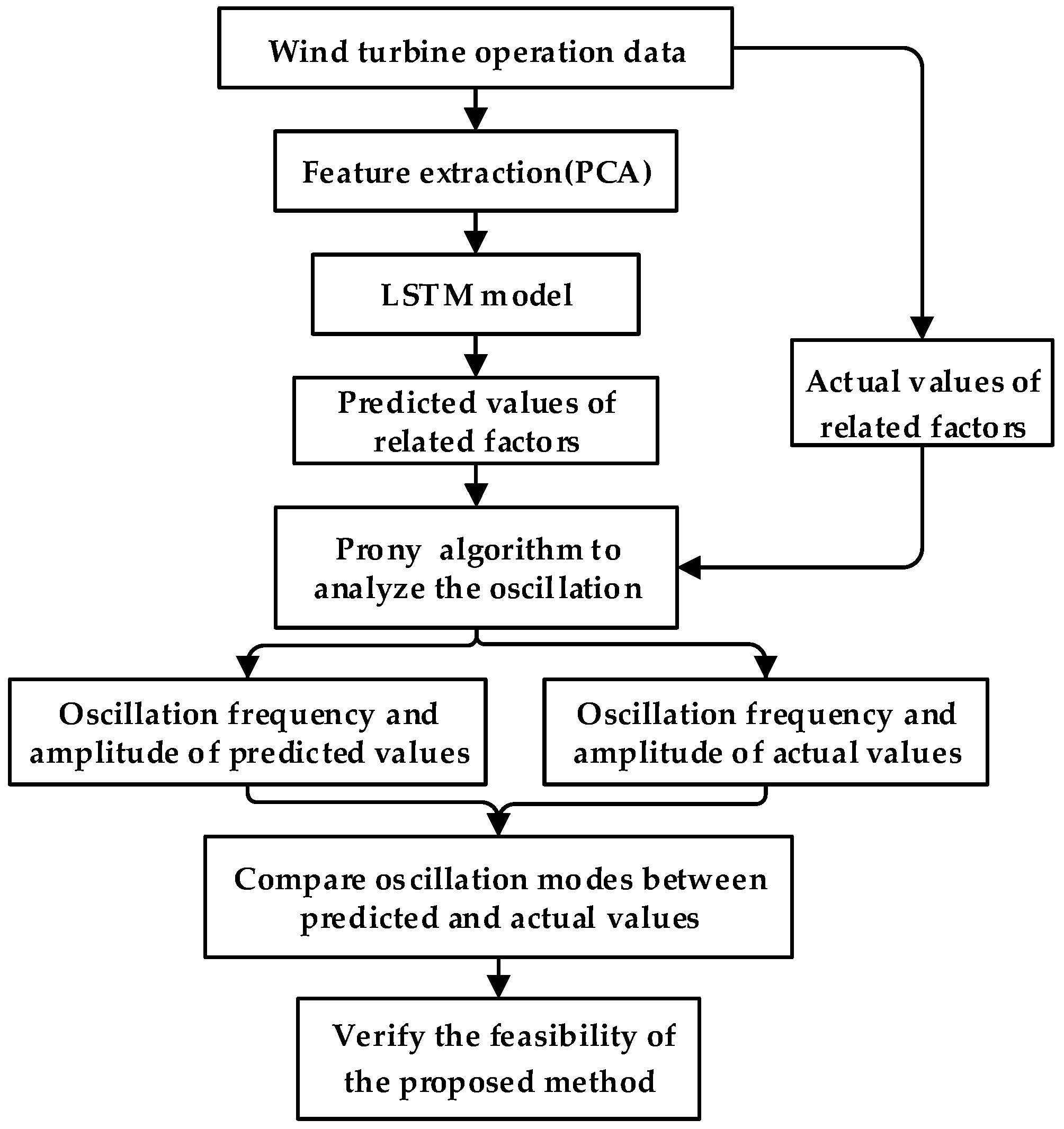
The first part of the article puts forward the related factors of wind turbine-grid interaction and introduces the PCA analysis. In the second part, the prediction model of wind turbine gird interaction is proposed, and the principle of LSTM network and the design scheme of prediction model are introduced. The third part introduce the data flow diagram of the model in TensorFlow. The fourth part is experimental verification and result analysis, which verifies the accuracy of the proposed model. Figure 1 shows the flowchart of the methodology used in this paper.

2. Selection of Related Factors of Wind Turbine Grid Interaction

2.1. Analysis Objects of Wind Turbine Grid Interaction

In this paper, wind output power, phase voltage and phase current are selected as the analysis objects of wind turbine grid interaction. First, it is necessary to build and train prediction models to predict power, voltage and current respectively. Too few predictors will lead to missing information and unable to conduct a comprehensive analysis of data. However, too many prediction factors will lead to an increase in the calculation amount and a decrease in the generalization ability, so it is necessary to select input features before prediction.

2.1.1. Voltage/Current

The factors that affect the voltage stability of wind turbines are usually the combination of various factors, including the scale of wind turbines, the type and size of disturbances, the type of generators and the operation mode of wind turbines. The harmonic of stator current is affected by stator and rotor voltages. In addition, the harmonic of stator current may also come from the wind motor itself, the disturbance of the surrounding environment, etc. Therefore, PCA will be used to select the input quantity that is related to the voltage and current.

2.1.2. Power

Wind turbine works by converting the kinetic energy in the wind first into rotational kinetic energy and then electrical energy, which can be supplied via the grid, the rotational kinetic power produced in a wind turbine is given by:

$$P_w=\frac{C_{p}S\rho v^3}{2}$$

(1)

In Equation (1), $P_w$ is the output power (kW), $C_p$ is the power coefficient, $\rho$ is air density (kg/m³), S is blade rolling area (m²), and $v$ is wind speed (m/s). Air density of the wind turbine is given by:

$$\rho =3.48\frac{p}{T}\left(1-0.378\frac{\phi P_b}{p}\right)$$

(2)

In Equation (2), $p$ represents normal atmospheric pressure level, $P_b$ is saturated vapor pressure, $T$ is thermodynamic temperature and $\phi$ is relative air humidity.

According to Equations (1) and (2), for a given wind turbine, the power coefficient and blade rolling area are constant, so the output power of the wind turbine is closely related to the following four factors: wind speed, temperature, humidity and pressure. Wind speed is the most important factor among them since it is a cubic parameter. Some of the above four factors are related to each other and some are independent of each other. As there is a certain correlation, it is possible to synthesize information existing in various variables with fewer factors. PCA belongs to this kind of dimensionality reduction method.

2.2. Principle of Principal Component Analysis

The idea of PCA [25] is to construct new variables formed by linear combination of original variables and make the new variables reflect as much information of the original variables as possible on the premise that they are not related to each other. Mapping n-dimensional features to k-dimensional (k < n), which is a completely new orthogonal feature, is called the main component. Principal components are reconstructed K-dimensional features, rather than simply removing the remaining N-K-dimensional features from the N-dimensional features. Each new feature has its own unique meaning. Data information is mainly reflected in variance. Features with large variance can reflect that the main information is contained in the original variables, usually measured by cumulative variance contribution rate. Generally, the dimension whose cumulative contribution rate is about 75~95% is selected.

There is a sample set $X=\{x_1,x_2,\dots ,x_{\mathrm{m}}\}$ assuming that the sample set is centered, that is ${\sum }_i{x}_{\mathrm{i}}=0$, assuming that the new coordinate system after projection transformation is $\{w_1,w_2,\dots ,w_{\mathrm{d}}\}$, where $w_i$ is the standard orthogonal basis vector, $\Vert w_{\mathrm{i}}\Vert {}_2=1$. The projection of the sample points $x_i$ on the hyperplane in the new space is $W^T{x}_{\mathrm{i}}$. In order for the projection of all the sample points to be separated as much as possible, the variance of the projected sample points should be maximized, and the variance of the projected sample points can be expressed as: ${\sum }_i{W}^T{x}_{\mathrm{i}}{x}_{\mathrm{i}}^{T}W$:

$$\underset{w}{\max }\mathrm{tr}\left(W^{T}X{X}^{T}W\right)\mathrm{s}.\mathrm{t}.W^{T}W=1$$

(3)

Applying the Lagrange multiplier method:

$$X{X}^{T}W=\lambda \mathrm{W}$$

(4)

Therefore, it is only necessary to perform eigenvalue decomposition on the covariance matrix $X{X}^T$ and sort the obtained eigenvalues: ${\lambda }_1\ge {\lambda }_2\ge \dots \ge {\lambda }_m$. The number of principal components selected depends on the cumulative variance contribution rate. Usually, when the cumulative variance contribution rate is greater than 75~95%, the corresponding previous p principal component contains most of the information that can be provided by the original variables m, and the number of principal components is just one. Variance contribution rate and cumulative variance contribution rate are respectively:

$${\eta }_i=\frac{100\%{\lambda }_i}{{\sum }_m{\lambda }_i}$$

(5)

$${\eta }_{\sum }(\mathrm{p})=\sum _i^p{\eta }_i$$

(6)

The solution of PCA is to form $\mathrm{W}=\{w_1,w_2,\dots ,w_{\mathrm{p}}\}$ corresponding to the previous eigenvalues.

3. Prediction Model of Analysis Objects in Wind Turbine Grid Interaction

3.1. Long-Term and Short-Term Memory Network Structure

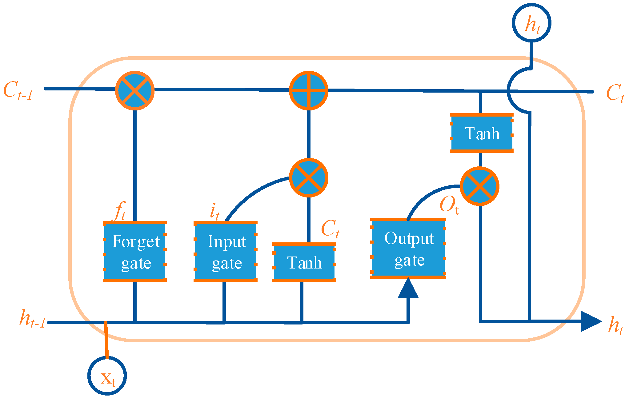
LSTM can be used as a complex nonlinear unit to construct a larger deep neural network, which can reflect the long-term memory effect. The LSTM network includes an input layer, an output layer, and multiple hidden layers. The hidden layer is composed of memory tuples, and its basic structure is shown in Figure 2. The key to LSTM network is cell state. The state of the cells runs directly along the whole chain like a conveyor belt. In LSTM, cell state information is added or deleted through the gate structure, and whether information passes through can be selectively determined through the gate. It consists of a Sigmoid layer and a pair of multiplication operations. The output of gate structure is 0~1, which defines the degree of information passing through. The tanh layer in Figure 2 is an activation function that can map a real number input into [−1, 1].

The LSTM tuple includes three gates, namely, an input gate, a forget gate and an output gate. The three gates control the flow of information between the tuple and the network. In the following formula, $i_{\mathrm{t}}$, $o_{\mathrm{t}}$, $f_{\mathrm{t}}$ represent the state values of input gate, output gate and forgotten gate, respectively.

(1)

Forget gate decides to forget information from the old cell state $C_{t-1}$, and the input is the input of the current layer $x_{\mathrm{t}}$ and the output of the previous layer $h_{t-1}$, the cell state output is:

$$f_t=\sigma \left(W_1^f·x_t+W_h^f·h_{t-1}+b_f\right)$$

(7)

(2)

Generate information to be updated and store it in the cell needs two steps: (a) update the information by the result of the input gate passing through the sigmoid layer; (b) $C_t$ will be added to the new candidate information by multiplying the old cell state with $f_t$ to forget unnecessary information:

$$i_t=\sigma \left(W_1^i·x_t+W_h^i·h_{t-1}+b_i\right)$$

(8)

$${\tilde{C}}_t=\tanh (W_1^C·x_t+W_h^C·h_{t-1}+b_C)$$

(9)

$$C_t=i_t\ast {\tilde{C}}_t+f_t\ast C_{t-1}$$

(10)

(3)

The output information is determined by the output gate. First, the initial output is obtained through the Sigmoid layer, the cell state value is scaled between [−1, 1] with the tanh layer, and the output $h_t$ can be easily obtained:

$$o_t=\sigma \left(W_1^o·x_t+W_h^o·h_{t-1}+b_o\right)$$

(11)

$$h_t=o_t\times \tanh \left(C_t\right)$$

(12)

From Equations (7) to (11), $W_1^i$, $W_1^f$, $W_1^o$, $W_1^C$ respectively represent the weight matrix of input gate, forget gate, output gate and tuple input, $W_{\mathrm{h}}^i,W_{\mathrm{h}}^f,W_{\mathrm{h}}^o,W_{\mathrm{h}}^C$ respectively represent the weight matrix of input gate, forgetting gate, output gate and tuple input to connect $h_{t-1}$, and $b_i,b_f,b_o,b_C$ respectively represent the bias vectors of input gate, forget gate, output gate and tuple input. $\sigma$ represents sigmoid activation function.

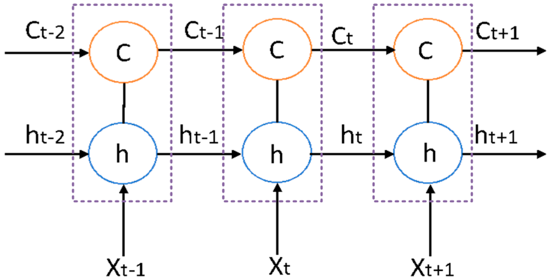
The LSTM model has the same structure as RNN model. It can be seen as multiple replications of the same neural network, and each neural network module will pass the message to the next one. After unfolding the loop, the structure is shown in Figure 3.

The observation objects of wind turbine network interaction and wind speed data is the input to the LSTM model, and the expression of the prediction model can be derived from the network structure of Figure 3:

$$h(t+1)=f(h(t),h(t-1),\dots ,h(t-n),x(t+1),x(t),\dots ,x(t-n))$$

(13)

In Equation (13), $h\left(t\right),\dots ,h\left(t-n\right)$ is the historical data, $x\left(t+1\right),\dots ,x\left(t-n\right)$ is the input parameter selected by PCA, in this case, it is wind speed.

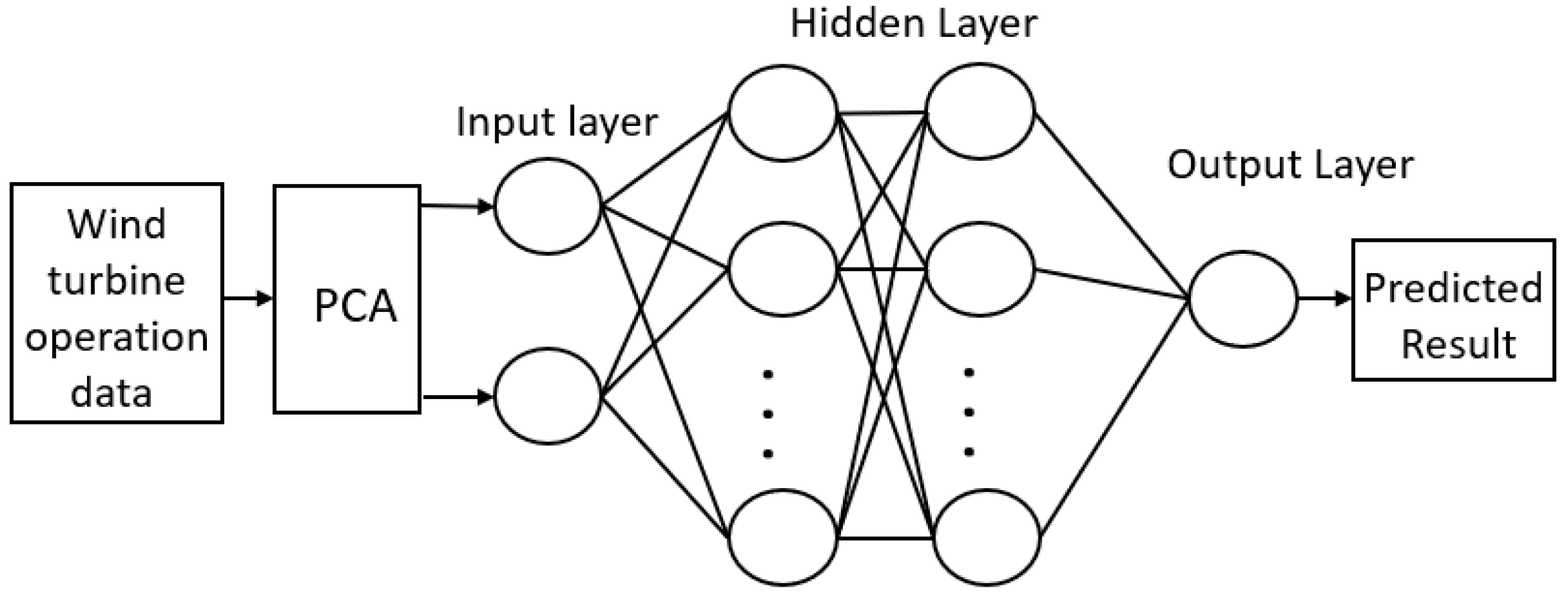
The topological structure of LSTM model selected in this paper is shown in Figure 4. After the principal component analysis of the original data, the analysis objects of wind turbine grid interaction and the selected principal component are chosen as inputs of the prediction model. We have two hidden layers. And the output layer gives the prediction of wind power, voltage and current in wind turbine grid interaction.

3.2. LSTM Prediction Model Design

3.2.1. Data Normalization

When predicting multi-variable time series, due to the different dimensions and numerical differences among different variables, considering the input and output range of nonlinear activation function in the model, and in order to equally handle the influence of various variables on wind power, voltage and current, it is necessary to normalize the raw data between [0, 1]. Normalization is carried out by MinMaxScaler, the formula is shown in Equation (14):

$$X_{std}=\frac{x-x.\min }{x.\max -x.\min }$$

(14)

The predicted wind power, current and voltage data are subjected to inverse normalization processing to make them have physical significance. The formula is shown in Equation (15):

$$X_{\mathrm{scaler}}={\mathrm{x}}_{std}(x.\max -x.\min )+x.\min$$

(15)

3.2.2. Model Parameter Selection

The establishment of LSTM prediction model requires five hyperparameters, namely, input dimension, input layer timesteps, number of hidden layers, dimension of each hidden layer and output dimension.

In an actual neural network, the number of hidden layers and neurons will directly affect the accuracy of network training and prediction so the number of hidden layers and neurons should be carefully selected. The network starts from a complex structure, which has many hidden layers and several hundred of neurons in each layer, then the over fitting problem happens, so that the number of layers should be reduced and some of the neurons should be dropped off until the generalization ability of the network is good enough, The best parameters for our model is found after many experiments, the following hyperparameters can obtain better prediction results: the input shape is 2, 5 time steps, the number of hidden layers is 2, 50 neurons are defined in the first hidden layer, 100 neurons are defined in the second hidden layer, and 1 neuron is defined in the output layer to predict the output. Adam function with random gradient descent is used as the optimization algorithm of the neural network.

3.2.3. Evaluation of Forecast Results

The mean absolute percentage error (MAPE) and root mean square error (RMSE) are used for evaluation the prediction results, and the error functions are shown in Equations (16) and (17), respectively:

$${\epsilon }_{MAPE}=\frac{1}{n}{\displaystyle \sum _{i=1}^n\frac{\left|{\widehat{P}}_N(i)-P_N(i)\right|}{P_N(i)}}\times 100\%$$

(16)

$${\epsilon }_{RMSE}=\sqrt{\frac{1}{n}{{\displaystyle \sum _{i=1}^n({\widehat{P}}_N(i)-P_N(i))}}^2}$$

(17)

In Equations (16) and (17), P_N(i) and ${\widehat{P}}_N(i)$ (i = 1, 2, 3, …, n) are the actual value and predicted value of the i th data, n represents the length of the data used for verification.

4. Model Implementation under Tensor Flow Framework

4.1. TensorFlow Framework

TensorFlow [26] is Google’s open source deep learning framework system, which supports a wide range of models and various types of learning algorithms. It can build deep learning models and can flexibly build analysis models as needed. TensorFlow uses data flow diagram to deal with numerical calculation. The nodes in the data flow diagram represent numerical operations, and the edges between nodes represent some connection between tensors, where tensors are represented by n dimensional arrays, flow is based on a data flow diagram, and tensor flow is the calculation process from one end of the graph to the other.

4.2. Construction of Tensor Flow Flow Diagram of the Model

Data flow diagram is an abstract description of computation. At the beginning of the calculation, the data flow graph is started in the session, which distributes the operations in the graph to each computing device while providing the execution method of the operations. These methods calculate and return tensors according to the calculation relationship of each side. The data flow diagram of the LSTM model constructed in this paper is shown in Figure 5, where the nodes are numerical operations and the edges are tensors represented by n dimensional arrays. The data flow diagram of the hidden layer is shown in Figure 6.

5. Result and Analysis

5.1. Data Preprocessing

The data used in this paper are collected from an actual wind farm. The sampling started at 13:33 on 6 August 2013 and ended at 14:03 on 6 August 2013. Since we are to research the interaction between the grid and wind farms, the sampling frequency should be very high and it is 4 kHz, that is, the data time interval is 1/4000 s, so there are in total 7,200,000 data items. The original data include factors such as fan speed, wind speed, wind direction, pressure, temperature, humidity and so on. If a certain factor is directly ignored, it may bring errors to the prediction. In order to reduce the dimension of input variables and minimize the errors, PCA is used to determine the minimum number of variables required and analyze the multivariate prediction factors.

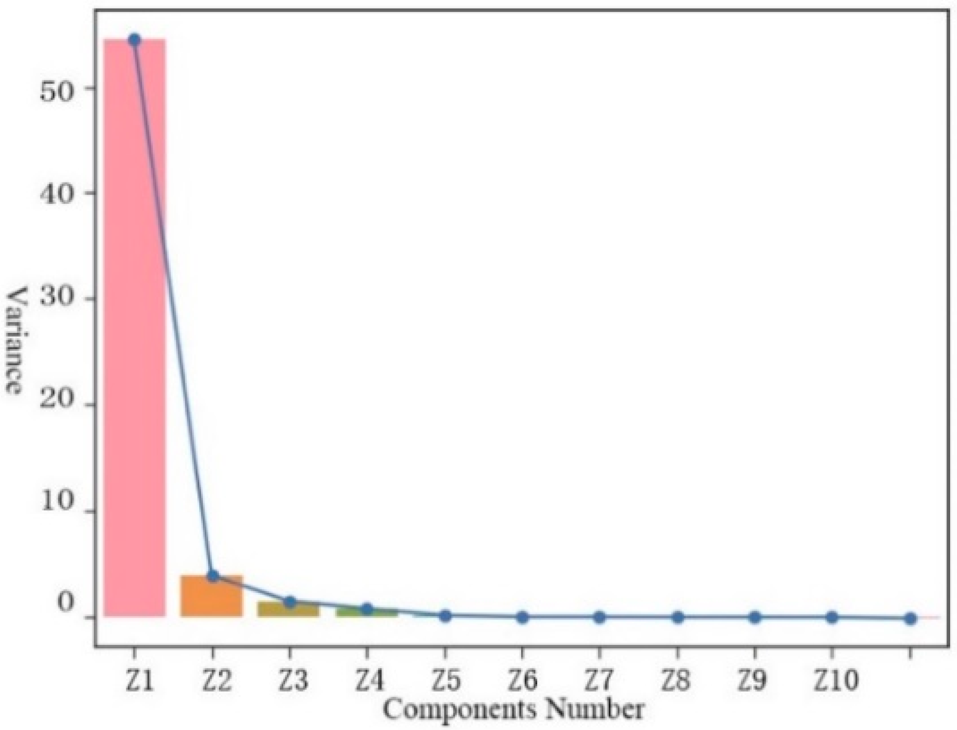
First, the data are normalized to unify the dimensions of each parameter, then principal component extraction is performed, the covariance matrix of the normalized training data is calculated, the characteristic root and contribution rate of the covariance matrix are calculated, and principal components are extracted according to the cumulative contribution rate. The calculation results are shown in

Table 1. Eigenvalues and contribution.

Principal Component	Eigenvalues	Variance Contribution Rate (%)	Cumulative Contribution Rate (%)
${\mathrm{Z}}_1$	11.917	89.273	89.273
${\mathrm{Z}}_2$	3.208	6.467	95.740
${\mathrm{Z}}_3$	1.994	2.500	98.240
${\mathrm{Z}}_4$	1.461	1.342	99.583
${\mathrm{Z}}_5$	0.669	0.281	99.865
${\mathrm{Z}}_6$	0.303	0.057	99.922
${\mathrm{Z}}_7$	0.274	0.047	99.969
${\mathrm{Z}}_8$	0.166	0.017	99.987
${\mathrm{Z}}_9$	0.130	0.010	99.997
${\mathrm{Z}}_{10}$	0.043	1.19 × 10−5	99.998

. Table 1 gives the eigenvalues, variance contribution rate and cumulative contribution rate of principal components, and Figure 7 is a line chart of variance relative to the number of components.

As can be seen from Table 1, the contribution rate of the first component ${\mathrm{Z}}_1$ is 89.273%, indicating that it basically contains all the information of the original data, and ${\mathrm{Z}}_1$ can be concluded as the principal component according to the principal component judgment. Another method of selecting principal components is to check the line chart of variance with respect to the number of components and select the point where the graph is close to the horizontal. From Figure 7, the graph is close to the horizontal after the first principal component and the contribution rate of other component variables is very low, so it is determined that the principal component is ${\mathrm{Z}}_1$. There are 10 input parameters before processing PCA, and only one principal component is used as a parameter after processing PCA.

As can be seen from the score of component coefficient matrix in

Table 2. Score of Component Coefficient Matrix.

Original Parameter Variable	Principal Component ${\mathbf{Z}}_1$
${\mathrm{X}}_1$	−0.011
${\mathrm{X}}_2$	0.001
${\mathrm{X}}_3$	−0.004
${\mathrm{X}}_4$	1.10 × 10−4
${\mathrm{X}}_5$	3.99 × 10−5
${\mathrm{X}}_6$	1.11 × 10−4
${\mathrm{X}}_7$	−0.089
${\mathrm{X}}_8$	0.965
${\mathrm{X}}_9$	−0.011
${\mathrm{X}}_{10}$	2.41 × 10−4

, this first principal component ${\mathrm{Z}}_1$ is mainly associated with the original parameter variable ${\mathrm{X}}_8$, with the correlation coefficient of 0.965, ${\mathrm{X}}_8$ corresponds to the wind speed. Therefore, the result obtained from the PCA is consistent with the result obtained from Equation (2) that wind speed is the most important influencing factor. The data preprocessing based on PCA can improve the calculation efficiency of the prediction model with guaranteed accuracy.

5.2. Results of Experimental Results

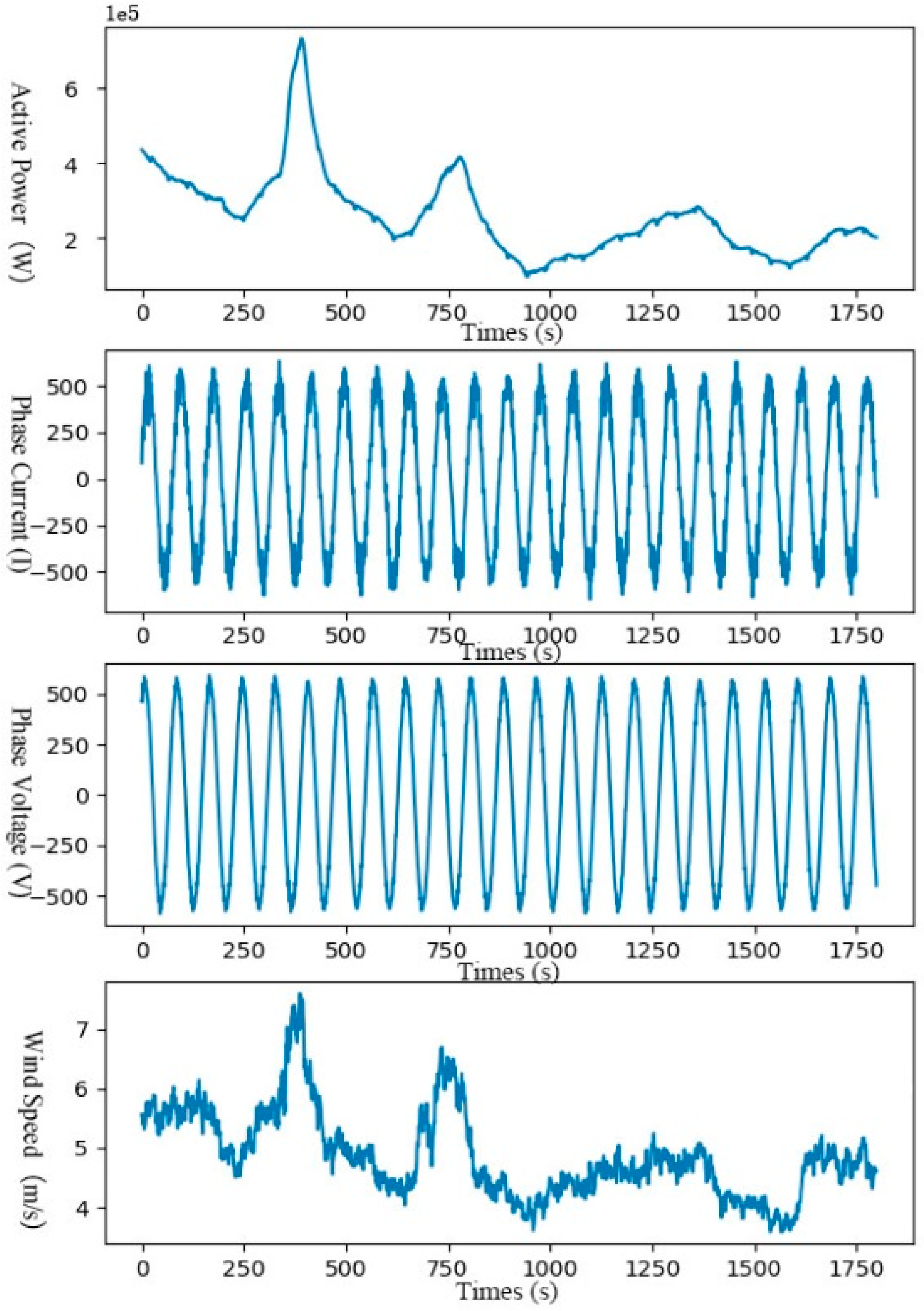
After implementing PCA, the selected parameters are treated as input to the model. Considering that the sampling frequency of the data is 4 kHz, to reduce the impact of individual data disturbance, an average method is adopted. The data used in the prediction is one point per second, that is, the average value of every 4000 data is taken as the current time value, and the average value is used for the processing of the output active power and wind speed. The waveforms of output active power, phase current, phase voltage is shown in Figure 8.

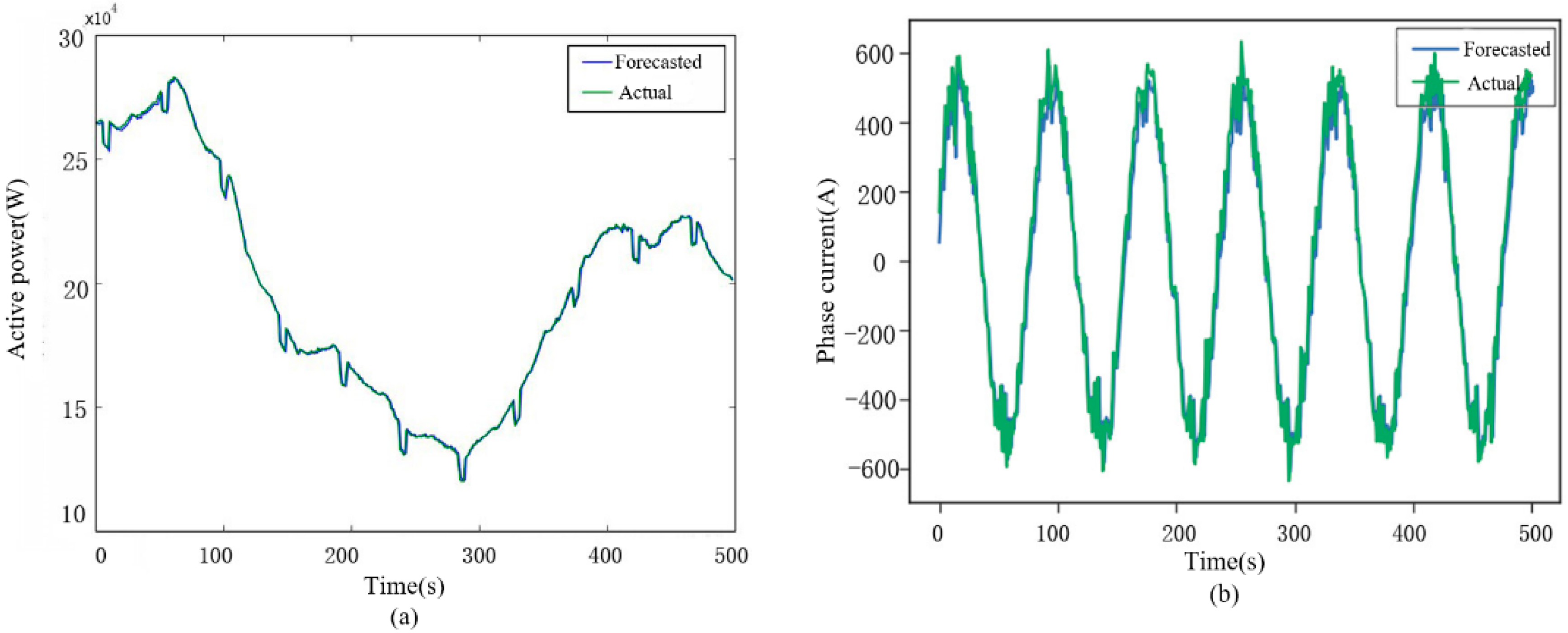
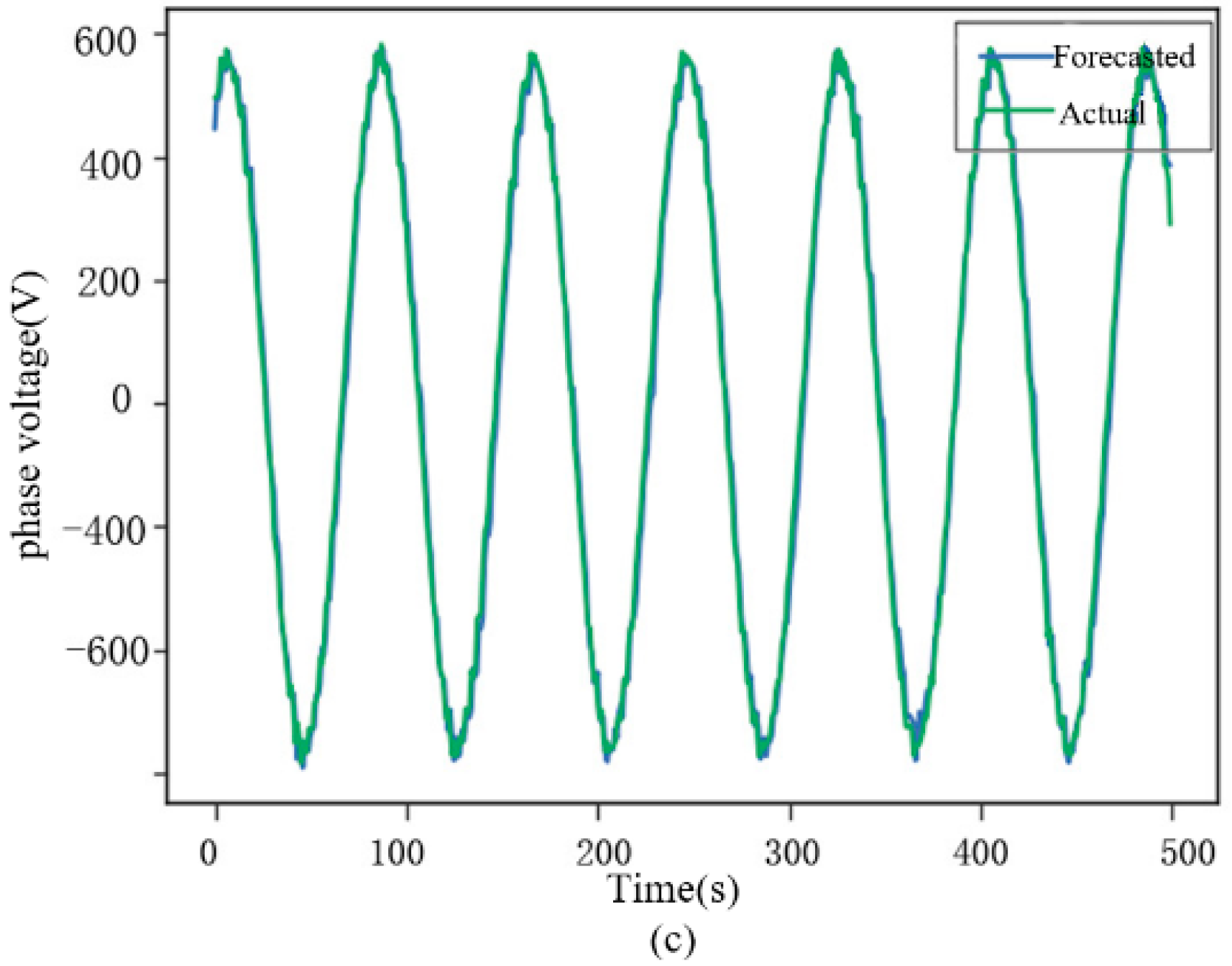
The pre-processed data are divided into training data and test data, where the training rate is defined as the proportion of training data to the total data. If the training rate is too high, the evaluation result may not be stable and accurate because the test set is too small. If the training rate is too low, the difference between the training set and the original data set will be too large to reduce the fidelity of the evaluation result. Generally, the training rate is set to [2/3, 4/5]. Here, the training rate is set to 0.72 because it satisfies the above requirements, that is, the data from 13:33 6 August 2013 to 13:54 6 August 2013 are taken as training samples. The target is to forecast the future 10 min’ wind farm operation data to verify the accuracy of LSTM network. As shown in Figure 9, the predicted results (a), (b) and (c) are a comparison of predicted and actual values of output power, phase current and phase voltage respectively. The blue line in the figure represents the predicted output and the green line represents the actual output.

From the prediction results in Figure 9a–c, the wind power, phase current and phase voltage prediction based on PCA-LSTM model have high accuracy and low prediction error. In Figure 9a, MAPE of wind power is 0.617%, RMSE is 2167.839, MAPE of phase current in Figure 9b is 3.287%, RMSE is 75.177, MAPE of phase voltage in Figure 9c is 2.383%, RMSE is 35.912. By predicting the output of the wind turbine, the peak load regulation and frequency modulation pressure of the power system can be relieved, mechanical failures can be found in time, corresponding measures can be taken as soon as possible, and the possibility of serious problems in the operation of the wind turbine can be reduced.

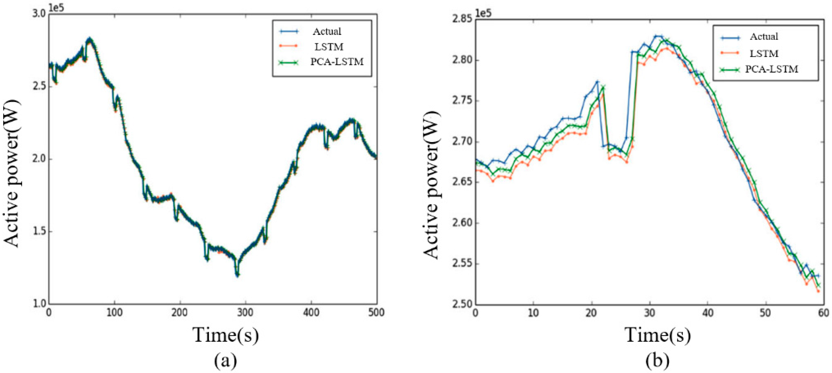
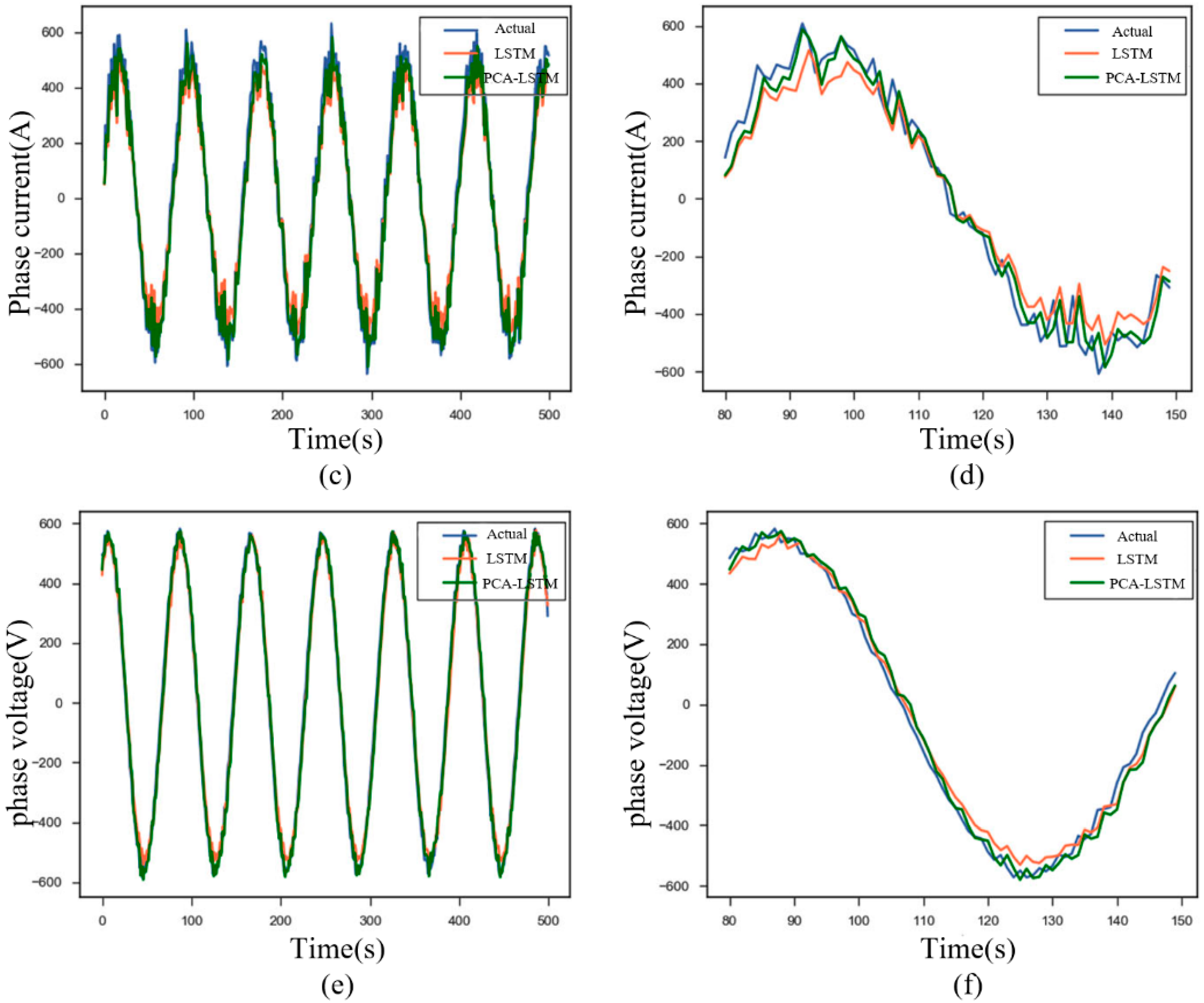
Figure 10a,c,e are the comparison of the prediction results of active power, phase current and phase voltage between PCA-LSTM model and single LSTM model proposed in this paper. Due to the large Y axis value, the comparison effect is not obvious enough, so Figure 10b,d,f are the typical fragments extracted from Figure 10a,c,e, which show the comparison of the prediction results of the two models.

As can be seen from Figure 10, the prediction results of LSTM and PCA-LSTM methods are close to the actual wind power, phase current and phase voltage curves, respectively, and the prediction accuracy of PCA-LSTM is higher than that of a single LSTM model, so the role of PCA in this prediction is very important. As can be seen from

Table 3. Error analysis of forecasting result.

		MAPE (%)	RMSE
Active Power	LSTM	0.703	2294.820
	PCA-LSTM	0.617	2167.839
Phase Current	LSTM	3.718	80.733
	PCA-LSTM	3.287	75.177
Phase Voltage	LSTM	2.515	37.841
	PCA-LSTM	2.383	35.912

, the RMSE of the PCA-LSTM model proposed in this paper is 5.533%, 6.887% and 5.098% lower than LSTM model, respectively.

By comparing the prediction results of single LSTM model and PCA-LSTM model, it shows that the higher the correlation degree with the target variables, the higher the prediction performance of LSTM model will be. On the contrary, variables with low correlation degree will not only affect the calculation speed, but may also reduce the prediction performance. This result shows that data preprocessing based on PCA increases the accuracy by 12.233% compared with the model using all variables as input parameters. Moreover, the input variables of PCA-LSTM model are much less than those of single LSTM model, which has the advantage of high computational efficiency in the case of large amount of data.

5.3. Comparison with Other Models

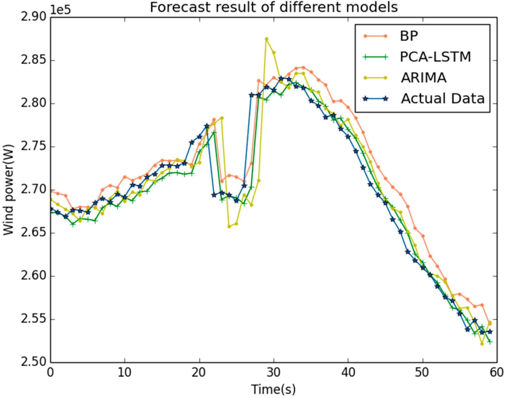
In this paper, a Relu function is used as activation function of LSTM network. In order to test performance of the network proposed in this paper, we compare it with classic time series prediction models such as BPNN model and ARIMA model, the output power is taken as the comparison object here. BPNN is a multi-layer feed-forward network trained according to back propagation. And the basic idea is gradient descent method. By analyzing the autocorrelation function and partial autocorrelation function of the residual, the optimal ARIMA model is determined as ARIMA (1,1,1). The prediction results are shown in Figure 11, the average absolute error percentage and root mean square error are shown in Table 3, respectively.

As can be seen from Figure 11, the predicted value obtained by the PCA-LSTM method proposed in this paper is closest to the actual value, and the prediction accuracy is higher than that based on BPNN model and ARIMA model. As can be seen from

Table 4. Error analysis of forecasting result.

Model	MAPE (%)	RMSE
ARIMA	1.397	3279.635
BP	3.127	6188.833
PCA-LSTM	0.617	2167.839

, the prediction error of the PCA-LSTM model is the lowest among the three models, and its MAPE is reduced by 2.510% and 0.780% compared with BPNN model and ARIMA model, respectively.

5.4. Analysis of the Interaction between Wind Turbine and Power Grid Based on the Predicted Values of Wind Turbines

In the experiments described in Section 5.2 and Section 5.3, it was confirmed that the prediction based on PCA-LSTM model has high accuracy, so it is reasonable to use the predicted value of the wind turbine-network interaction observation object as the basis for judging the operation state of the system.

The prediction data and the actual data within a certain time period are selected, and Prony algorithm is used to analyze the oscillation module. The analysis results are shown in

Table 5. The analysis results of the actual value and forecast value based on Prony algorithm.

Analysis Variables	Predicted Values		Acutal Values
	Amplitude	Frequency	Amplitude	Frequency
Phase Voltage	548.430	49.997	556.963	50.005
	15.629	93.446	24.324	97.834
	14.565	5.793	21.938	7.165
	7.921	57.075	7.962	49.217
	5.146	31.684	6.370	31.592
	5.060	15.129	6.151	17.050
	3.803	29.467	4.814	81.116
	12.656	23.524	12.345	26.718
	14.672	86.070	10.771	72.889
	15.201	99.686	32.395	94.986
Phase Current	536.425	49.982	502.094	49.948
	108.699	99.199	218.504	89.113
	99.337	92.721	23.097	86.005
	44.119	35.084	33.958	35.348
	20.349	43.825	39.743	42.536
	15.561	79.743	70.394	80.881
	12.364	27.780	17.493	25.034
	19.438	13.220	47.057	11.331
	36.879	25.695	17.541	27.364
	32.085	0.7709	16.690	0.5920
Active Power	45,546.265	93.741	11,189.343	97.706
	38,424.916	14.442	8693.302	16.870
	37,029.951	43.067	3342.516	46.448
	20,930.455	68.097	7387.538	81.205
	26,593.189	26.526	6691.952	27.803
	45,624.802	54.818	1424.351	52.505
	43,840.524	48.451	905.538	49.885
	25,240.689	64.235	1744.815	70.239
	49,782.074	35.610	1375.600	39.525
	31,739.939	12.097	2583.231	8.693

. In addition, the oscillation frequency of the turbine-grid interaction is between 0 and 100 Hz, so the oscillation frequency higher than 100 Hz is eliminated. From the above data, it can be concluded that subsynchronous control interaction (SSCI), subsynchronous oscillation (SSO) and subsynchronous resonance (SSR) exist during the actual system operation, and the frequency value and actual value of the predicted data output by LSTM model are also similar, with subsynchronous oscillation and subsynchronous resonance as the main oscillation components.

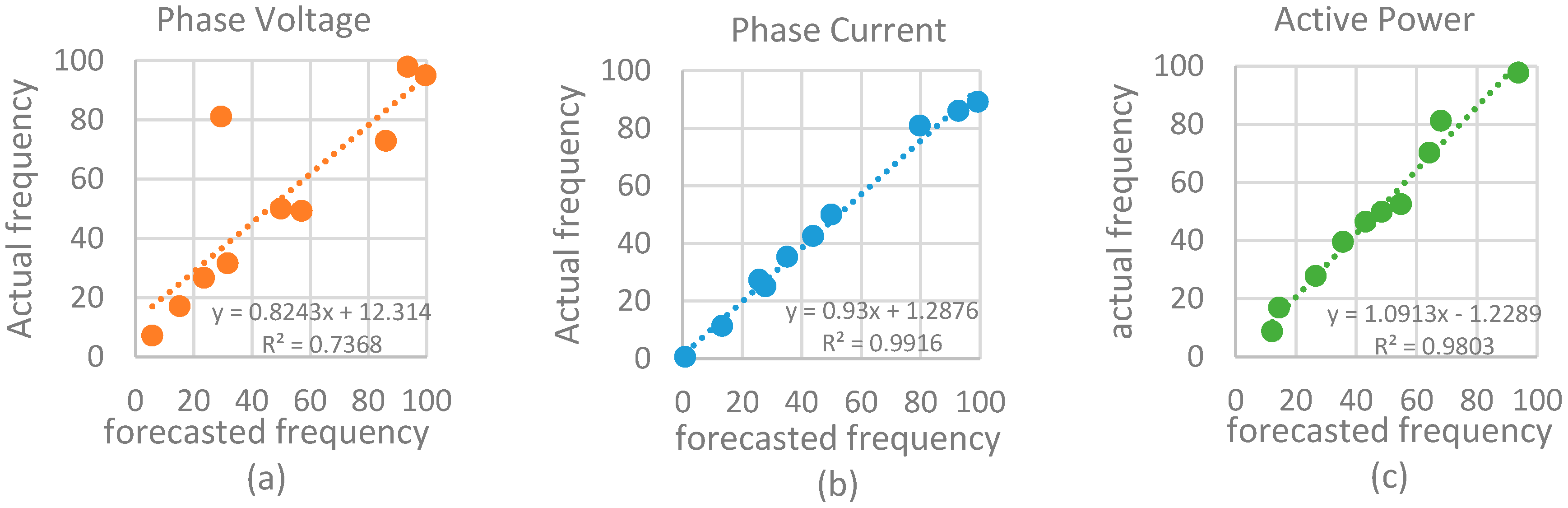
Based on the analysis of the actual operation data of wind turbines, it is found that several oscillation modes such as low-frequency oscillation, subsynchronous control interaction (SSCI), subsynchronous oscillation (SSO) and subsynchronous resonance (SSR) exist in the actual system operation, but due to various factors, the frequency value will be slightly different from the theoretical calculated characteristic frequency value. The output current, voltage and power of wind turbines mainly include frequency values of 0.8, 8, 12, 25, 45, 50 and 90 Hz. As shown in Figure 12a–c, the X axis is the frequency component obtained from the LSTM-PCA model, the Y axis is the frequency component obtained from the actual active power, and Figure 13 is a hexagonal box diagram drawn from the above three charts, which more visually depicts the relationship between the predicted power and the actual power. the darker the hexagon, the more frequent the certain frequency component appears, so it shows that the frequency component of 12, 25 and 50 Hz appears more often. From Figure 13, it shows that the frequency value of the predicted data output by PCA-LSTM model is basically the same as the actual frequency value.

Table 6. Analysis of Oscillation Mode of Wind Turbine on Forecasted Phase Current, Phase voltage and Power.

Observation Object\Oscillation Mode		SSO	SSR	SSCI	Low-Frequency Oscillation
Phase Current	Frequency	13.220	25.695	5.793	/
Phase Voltage		15.129	23.524	/	0.771
Active Power		14.442	26.526	/	/

and

Table 7. Analysis of Oscillation Mode of Wind Turbine on Actual Phase Current, Phase voltage and Power.

Observation Object\Oscillation Mode		SSO	SSR	SSCI	Low-Frequency Oscillation
Phase Current	Frequency	11.331	25.034	/	0.592
Phase Voltage		17.050	26.718	7.165	/
Active Power		16.870	27.803	8.693	/

are respectively the oscillation modes corresponding to the predicted phase current, phase voltage and active power of the wind turbine and the oscillation modes corresponding to the actual phase current, phase voltage and active power of the wind turbine.

According to Table 6 and Table 7, there are many components in subsynchronous oscillation and subsynchronous resonance of wind turbines, and there is a greater possibility of excitation. Low-frequency oscillation mainly exists in phase current and phase voltage, and the possibility of excitation is relatively small. The experiment of the above measured data fully verifies the feasibility and high accuracy of the analysis of the interaction between the grid and wind turbine based on the predicted values of phase current, phase voltage and active power of the wind turbine base on PCA-LSTM model. Based on the predicted values of phase current, phase voltage and active power of wind turbines, it is possible to control the possible interaction between grid and wind turbine in time by analyzing the operating state of the system, which is of great significance to the safe operation of the grid.

6. Conclusions

In this paper, a prediction model of wind turbine-grid interaction based on LSTM network is proposed under TensorFlow. When selecting the model input variables, PCA is used to select appropriate input variables, which reduces the data dimension. On the analysis of oscillation mode, the prediction data of the interaction between wind turbine and grid are analyzed by Prony algorithm. By analyzing the measured data of a wind turbine, the following conclusions are obtained:

(1)

PCA can reduce the dimensions of input variables, reflect the main factors affecting wind power prediction, and improve the operation speed on the premise of ensuring the prediction accuracy. Compared with the single LSTM model, the prediction accuracy of PCA-LSTM is obviously improved. In terms of wind power, phase current and phase voltage prediction, RMSE of PCA-LSTM model is reduced by 5.533%, 6.887% and 5.098%, respectively, compared with the LSTM model.

(2)

A LSTM network can effectively analyze massive amounts of data. Compared with the traditional time series prediction method, the deep learning method has the advantages of strong learning and generalization ability, and the performance increases with the increase of data size. Compared with other prediction methods, this method has higher accuracy and applicability. Compared with BPNN model and ARIMA model, its MAPE decreased by 2.510% and 0.780%, respectively.

(3)

Based on the actual data and the predicted data of the model, the oscillation modes of the interaction between the wind turbine and power grid are analyzed by Prony algorithm, which proves that the oscillation frequency of the predicted data from PCA-LSTM model proposed in this paper are basically the same as the oscillation frequency of the actual data, and from the oscillation frequency, it is found that wind turbines have more harmonic components such as 12, 25 and 50 Hz, that is, there are more sub synchronous oscillations and sub synchronous resonances, and there is a greater possibility of being stimulated, which verifies the feasibility of the proposed method for analyzing the interaction between wind turbines and power grid.

(4)

In this paper, the active power, phase current and phase voltage are selected as the related objects of the interaction between wind turbine and grid. The effectiveness of the method, which based on the predicted value of the related objects to analyze the amplitude and frequency of the interaction, is verified by experiment on actual data. Prediction of operational status has laid a solid foundation for future work, which is the timely management of the interaction between wind turbine and grid.

References

- Lu, Y.; Xie, D.; Sun, J.; Lou, Y.; Zhang, Y.; Wang, X. Modeling and Simulation of Small Signal Torsional Vibration of Wind Farms. Power Syst. Technol. 2016, 40, 1120–1127. [Google Scholar] [CrossRef]
- Xu, Q.; He, D.; Zhang, N.; Kang, C.; Xia, Q.; Bai, J.; Huang, J. A Short-Term Wind Power Forecasting Approach With Adjustment of Numerical Weather Prediction Input by Data Mining. IEEE Trans. Sustain. Energy 2015, 6, 1283–1291. [Google Scholar] [CrossRef]
- Xue, Y.; Yu, C.; Zhao, J.; Li, L.; Liu, X.; Wu, Q.; Yang, G. A Review on Short- term and Ultra-short-term Wind Power Prediction. Autom. Electr. Power Syst. 2015, 39, 141–151. [Google Scholar]
- Guan, C.; Luh, P.B.; Michel, L.D.; Chi, Z. Hybrid Kalman Filters for Very Short-Term Load Forecasting and Prediction Interval Estimation. IEEE Transa. Power Syst. 2013, 28, 3806–3817. [Google Scholar] [CrossRef]
- Chen, X.W.; Lin, X. Big Data Deep Learning: Challenges and Perspectives. IEEE Access 2014, 2, 514–525. [Google Scholar] [CrossRef]
- Dong, B.; Yang, B. Prediction of short-term wind power based on LSSVM. Hydropower New Energy 2017, 7, 76–78. (In Chinese) [Google Scholar] [CrossRef]
- Fan, G.; Wang, W.; Liu, C.; Dai, H. Wind Power Prediction Based on Artificial Neural Network. Proceed. CSEE 2008, 28, 118–123. [Google Scholar] [CrossRef]
- Barbounis, T.G.; Theocharis, J.B.; Alexiadis, M.C.; Dokopoulos, P.S. Long-term wind speed and power forecasting using local recurrent neural network models. IEEE Trans. Energy Conver. 2006, 21, 273–284. [Google Scholar] [CrossRef]
- Hochreiter, S.; Bengio, Y.; Frasconi, P.; Schmidhuber, J. Gradient flow in recurrent nets: The difficulty of learning long-term dependencies. In A Field Guide to Dynamical Recurrent Networks; Wiley-IEEE Press: Hoboken, NJ, USA, 2001; pp. 237–243. [Google Scholar]
- Mandal, P.; Srivastava, A.K.; Park, J.W. An Effort to Optimize Similar Days Parameters for ANN-Based Electricity Price Forecast. IEEE Trans. Ind. Appl. 2009, 45, 1888–1896. [Google Scholar] [CrossRef]
- Archer, C.L.; Simão, H.P.; Kempton, W.; Powell, W.B.; Dvorak, M.J. The challenge of integrating offshore wind power in the U.S. electric grid. Part I: Wind forecast error. Renew. Energy 2017, 103, 346–360. [Google Scholar] [CrossRef]
- Jurasz, J.; Mikulik, J.; Krzywda, M.; Ciapała, B.; Janowski, M. Integrating a wind- and solar-powered hybrid to the power system by coupling it with a hydroelectric power station with pumping installation. Energy 2018, 144, 549–563. [Google Scholar] [CrossRef]
- Kies, A.; Schyska, B.; Viet, D.T.; Bremen, L.V.; Heinemann, D.; Schramm, S. Large-scale integration of renewable power sources into the Vietnamese power system. Energy Procedia 2017, 125, 207–213. [Google Scholar] [CrossRef]
- Ming, B.; Liu, P.; Guo, S.; Cheng, L.; Zhou, Y.; Gao, S.; Li, H. Robust hydroelectric unit commitment considering integration of large-scale photovoltaic power: A case study in China. Appl. Energy 2018, 228, 1341–1352. [Google Scholar] [CrossRef]
- Jurasz, J. Modeling and forecasting energy flow between national power grid and a solar–wind–pumped-hydroelectricity (PV–WT–PSH) energy source. Energy Conver. Manag. 2017, 136, 382–394. [Google Scholar] [CrossRef]
- Dobson, I.; Zhang, J.; Greene, S.; Engdahl, H.; Sauer, P.W. Is Strong Modal Resonance a Precursor to Power System Oscillations. IEEE Trans. Circuits Syst. 2001, 48, 340–349. [Google Scholar] [CrossRef]
- Li, M.; Yu, Z.; Xu, T.; He, J.; Wang, C.; Xie, X.; Liu, C. Study of Complex Oscillation Caused by Renewable Energy Integration and Its Solution. Power Syst. Technol. 2017, 41, 1035–1042. [Google Scholar] [CrossRef]
- Yu, Y.; Shen, Y.; Zhang, X.; Zhu, J.; Du, J. The load oscillation energy and its effect on low-frequency oscillation in power system. In Proceedings of the 2015 5th International Conference on Electric Utility Deregulation and Restructuring and Power Technologies (DRPT), Changsha, China, 14 March 2016. [Google Scholar]
- Zhang, Z.; Liu, S.; Zhu, G.; Lu, Z. SSCI detection and protection in doubly fed generator based on DTFT. J. Eng. 2017, 13, 2104–2107. [Google Scholar] [CrossRef]
- Xie, X.; Wang, L.; He, J.; Liu, H.; Wang, C.; Zhan, Y. Analysis of Subsynchronous Resonance/Oscillation Types in Power Systems. Power Syst. Technol. 2017, 41, 1043–1049. [Google Scholar]
- IEEE Subsynchronous Resonance Working Group. Proposed terms and definitions for subsynchronous oscillations. IEEE Trans. Power Appar. Syst. 1980, PAS-99, 506–511. [Google Scholar] [CrossRef]
- Adams, J.; Carter, C.; Huang, S.-H. ERCOT experience with sub-synchronous control interaction and proposed remediation. In Proceedings of the PES T&D 2012, Orlando, FL, USA, 7–10 May 2012. [Google Scholar]
- Liu, H.; Xie, X.; Zhang, C.; Li, Y.; Liu, H.; Hu, Y. Quantitative SSR analysis of series-compensated DFIG-based wind farms using aggregated RLC circuit model. IEEE Trans. Power Syst. 2017, 32, 474–483. [Google Scholar] [CrossRef]
- Fan, L.; Kavasseri, R.; Miao, Z.L.; Zhu, C. Modeling of DFIG-Based Wind Farms for SSR Analysis. IEEE Trans. Power Deliv. 2010, 25, 2073–2082. [Google Scholar] [CrossRef]
- Bianchi, F.M.; De Santis, E.; Rizzi, A.; Sadeghian, A. Short-Term Electric Load Forecasting Using Echo State Networks and PCA Decomposition. IEEE Access 2015, 3, 1931–1943. [Google Scholar] [CrossRef]
- Wongsuphasawat, K.; Smilkov, D.; Wexler, J.; Wilson, J.; Mané, D.; Fritz, D.; Krishnan, D.; Viégas, F.B.; Wattenberg, M. Visualizing Dataflow Graphs of Deep Learning Models in TensorFlow. IEEE Trans. Vis. Comput. Graph. 2018, 24, 1–12. [Google Scholar] [CrossRef] [PubMed]
Figure 1.
Flowchart of the methodology.
Figure 2.
Cell structure of LSTM.
Figure 3.
Network structure unfolded in time.
Figure 4.
Topology structure of LSTM model.
Figure 5.
TensorFlow data flow diagram.
Figure 6.
Data flow diagram of hidden layer in LSTM model.
Figure 7.
The scatter of variance relative to the number of component.
Figure 8.
Waveform of raw data.
Figure 9.
Comparison of actual output and predicted output. (a) Active power; (b) Phase current; (c) Phase voltage.
Figure 10.
Forecast results and partial results of PCA-LSTM and LSTM. (a) Active power; (b) Partial active power; (c) Phase current; (d) Partial phase current; (e) Phase voltage; (f) Partial phase voltage.
Figure 11.
Prediction results between PCA-LSTM and ARIMA.
Figure 12.
Analysis results of the actual value and forecast value of actual phase current, phase voltage and power based on Prony algorithm (a) Phase voltage; (b) Phase current; (c) Active power.
Figure 13.
Jointplot of hex.