Adaptive-Observer-Based Data Driven Voltage Control in Islanded-Mode of Distributed Energy Resource Systems

Abstract

In this paper, an adaptive observer based data driven control scheme is proposed for the voltage control of dispatchable distributed energy resource (DER) systems which work in islanded operation. In the design procedure of the proposed control scheme, we utilize the novel transformation and linearization technique for the islanded DER system dynamics, which is proper for the proposed data driven control algorithm. Moreover, the pseudo partial derivative (PPD) parameter matrix can be estimated online by multiple adaptive observers. Then, the adaptive constrained controller is designed only based on the online identification results derived from the input/output (I/O) data of the controlled DER system. It is theoretically proven that all the signals in the closed-loop control system are uniformly ultimately bounded based on the Lyapunov stability analysis approach. In addition, the results of the simulation comparison are given to verify the voltage control effect of the proposed control scheme.

1. Introduction

Solar energy is clean, without pollution, and inexhaustible, so the application of solar energy has been a wide concern of the academic and industrial circles. In general, many remote areas and islands around the world are rich in solar energy. Therefore, it is conducive to build a micro-grid by forming a dispatchable photovoltaic (PV) distributed energy resource (DER) system. When the micro-grid works in islanded operation mode, the DER system can be used as the main power supply for micro-grid to provide voltage and frequency support which can sufficiently exert the advantage of the fast response of the DER system. However, one of the main challenges, is to keep the stability of the amplitude and frequency of micro-grid’s ac voltage under the unbalanced network conditions [1,2].

In general, islanded operation is not permitted under the present utility standards [3]. However, under the precondition that the DER system has the capacity to supply the total power of the local loads, the stand-alone islanded system can be applied [4,5,6]. In recent years, there has been much research on how to realize the fine control of the islanded DER system. In [6], the stability of voltage and frequency of the stand-alone DER system was maintained by adopting the proposed linear quadratic Gaussian controller which utilizes the technique of robust control. However, the response of the system output voltage was very slow, and the frequency of the output voltage was unstable. In [7], a novel unified controller was proposed for regulating the output voltage ofthe multibus micro-grid system. In addition, simulation by using the real-time digital simulator (RTDS) can verify the effectiveness of the proposed voltage control scheme. However, from the experimental waveform, it can be seen that the voltage waveform has great distortion and the output power of the system also has jitter. In [8], a control strategywas proposed for multiple DER systems which both operate in islanded mode. However, the systems obtained a favorable control effect only when the load had the characteristics of being linear and balanced. In order to reduce the influence of the load on the performance of the DER islanded system, the authors proposed a control method by adopting the techniques of feed-forward and decoupling compensation in [5]. However, the control strategy designed in this paper is based on PID control, and the output voltage of the system has a large static error when tracking the reference voltage. In [9], a control scheme based on the repetitive and deadbeat control was proposed for dispatchable electronically-interfaced DER islanded systems under the unbalanced load condition. However, the fluctuation of the current in the system seemed to have a great influence on the voltage, especially when the non-linear load was connected. Sliding mode control (SMC) has been successfully applied in power systems [10,11,12,13,14,15]. In [13], a fractional-order SMC strategy with black-start ability was designed to improve the quality of the output ac voltage of the host DER islanded systems. In [14], a modified terminal sliding-mode control (TSMC) with integral compensation method was proposed as a way of controlling the voltage-sourced converter (VSC) which drives varying loads. In [15], an adaptive robust total sliding-mode control (ARTSMC) scheme was proposed to stabilize the voltage and frequency of the micro-grid. Moreover, the proposed ARTSMC scheme has good control performance between the two operation modes (grid-connected mode and off-grid mode). However, most of the control strategies for DER systems studied at present are model-based control strategies and their control effects depend on the accuracy of the dynamic model.

With the development of technology, the performance of control system has become increasingly demanding. The excellent integrated control methods are getting more and more attention. Different from traditional control, the new methods require little model information and can be computed online easily. Therefore, control methods based on the data-driven approach were proposed in this background [16,17,18]. Model-free adaptive control (MFAC), one of the data-driven control (DDC) methods, has been studied by some scholars [17,19,20,21,22]. In [23], an improved MFAC algorithm was proposed for the coordination design of a wide-area power system stabiliser (WAPSS) to ensure the cooperation of the controllers under different operating conditions without tedious system modelling. In [24], the authors proposed a distributed MFAC scheme for multi-agent systems to solve consensus tracking problems only by using the input/output (I/O) data of each agent. Theoretical analysis, simulation, and practical application proved that the MFAC method has the advantages of strong robustness, small computational burden and easy implementation [19,20,21,25,26].

In this paper, we propose a novel data-driven MFAC method based on the multiple adaptive observer technique to accommodate the multi-input multi-output (MIMO) DER system. The design of the proposed method only depends on the I/O data of the MIMO controlled plant. Compared with other control methods, the MFAC method does not depend on the information from an accurate dynamic model, thus avoiding the control effect deterioration caused by an incomplete model. Moreover, the pseudo partial derivative (PPD) parameter matrix can be estimated online by the multiple adaptive observer. Then, the adaptive constrained controller is designed based on the online identification of multiple observer to solve the control input rate constraint problem of DER system. The simulation and comparison results are given to verify the superiority of the proposed method. The major contributions and innovations of this paper are displayed as follows.

• The model-free control method is applied to the voltage control of the DER system, which reduces the dependence of the controller on model information.
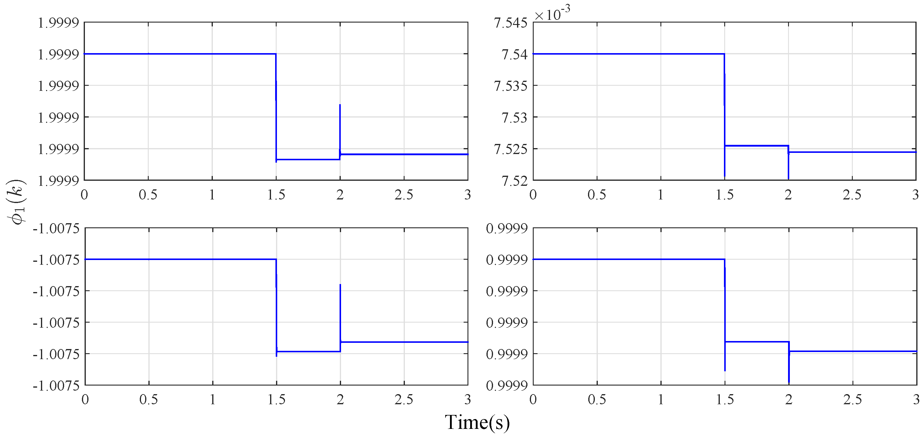
• The PPD parameter estimation algorithm is designed based on the multiple observer technique, which can guarantee the errors of observation converge to 0.
• We utilize the novel transformation and linearization technique for the islanded DER system dynamics. The main advantage of this method is that the dynamics of the MIMO DER system are transformed and linearized properly for the proposed MFAC algorithm.
• By constructing the Lyapunov function, it is theoretically proven that all the signals in the closed-loop control system are bounded.

The rest of this paper is organized as follows. In Section 2, the mathematical model of the DER islanded system is given. Then, we utilize the novel transformation and linearization technique for the islanded DER system dynamics, which is proper for the following proposed MFAC algorithm. In Section 3, the multiple observer-based data-driven model-free adaptive constrained control scheme and the proof of stability for control system are presented. In Section 4, simulation results and comparisons are given to demonstrate the effectiveness of the proposed MFAC scheme. Finally, we summarize the conclusions in Section 5.

2. Dynamics Transformation and Linearization of Islanded DER System

2.1. Mathematic Model of the Islanded DER System

As shown in Figure 1, the dynamics of the islanded DER system can be expressed as the space-phasor equations, as follows [13]:

$$\begin{array}{c}C\frac{d{\overrightarrow{U}}_x}{dt}=\overrightarrow{I}-{\overrightarrow{I}}_x\hfill \end{array}$$

(1)

$$\begin{array}{c}{L}_s\frac{d\overrightarrow{I}}{dt}={\overrightarrow{U}}_v-{\overrightarrow{U}}_x-R\overrightarrow{I}\hfill \end{array}$$

(2)

where ${\overrightarrow{U}}_x$, $\overrightarrow{I}$, ${\overrightarrow{I}}_x$ and ${\overrightarrow{U}}_v$ are defined as the space phasor corresponding to $U_{xabc}$, $I_{abc}$, $I_{xabc}$ and $U_{vabc}$, respectively.

In view of (1), (2) and Equation ${\overrightarrow{U}}_v=(U_{dc}/2)\overrightarrow{\tau }$, which is related to the PWM modulating signals (${\tau }_{abc}$) of the VSC, we can obtain

$$\begin{array}{c}\hfill \frac{d^2{\overrightarrow{U}}_x}{d{t}^2}=\frac{U_{dc}\overrightarrow{\tau }}{2L_{s}C}-\frac{R}{L_s}\frac{d{\overrightarrow{U}}_x}{dt}-\frac{{\overrightarrow{U}}_x}{L_{s}C}-\frac{1}{C}\frac{d{\overrightarrow{I}}_x}{dt}-\frac{R{\overrightarrow{I}}_x}{L_{s}C}.\end{array}$$

(3)

Express (3) in the case of its $dq$ components. Then, Equation (3) can be split into (4) and (5), where w denotes the frequency of all the $abc$-frame variables:

$$\begin{array}{c}\hfill \frac{d^2{U}_{xd}}{d{t}^2}=2w\frac{d{U}_{xq}}{dt}-\frac{R}{L_s}\frac{d{U}_{xd}}{dt}+\left(w^2-\frac{1}{L_{s}C}\right)U_{xd}+\frac{Rw}{L_s}{U}_{xq}-\frac{1}{C}\frac{d{I}_{xd}}{dt}+\frac{w}{C}{I}_{xq}-\frac{R}{L_{s}C}{I}_{xd}+\frac{U_{dc}}{2L_{s}C}{\tau }_d\end{array}$$

(4)

$$\begin{array}{c}\hfill \frac{d^2{U}_{xq}}{d{t}^2}=-2w\frac{d{U}_{xd}}{dt}-\frac{R}{L_s}\frac{d{U}_{xq}}{dt}+\left(w^2-\frac{1}{L_{s}C}\right)U_{xq}-\frac{Rw}{L_s}{U}_{xd}-\frac{1}{C}\frac{d{I}_{xq}}{dt}-\frac{w}{C}{I}_{xd}-\frac{R}{L_{s}C}{I}_{xq}+\frac{U_{dc}}{2L_{s}C}{\tau }_q.\end{array}$$

(5)

2.2. Dynamics Transformation and Linearization Technique

This section presents the novel transformation and linearization method of the islanded DER system dynamics, which is proper for the proposed MFAC scheme.

First, Equations (4) and (5) can be rewritten as the following state-space form:

$$\begin{array}{c}\hfill \ddot{\mathbf{U}}=M\dot{\mathbf{U}}+Z\tau +N\mathbf{U}+P\dot{\mathbf{I}}+Q{\mathbf{I}}^{\prime }\end{array}$$

(6)

where $\mathbf{U}={(U_{xd},U_{xq})}^T$, $\dot{\mathbf{I}}={({\dot{I}}_{xd},{\dot{I}}_{xq})}^T$, ${\mathbf{I}}^{\prime }={(I_{xq},I_{xd})}^T$, $\tau ={({\tau }_d,{\tau }_q)}^T={({\tau }_1,{\tau }_2)}^T$, $M=\left[\begin{array}{cc}-\frac{R}{L_s}& 2w\\ -2w& -\frac{R}{L_s}\end{array}\right]$, $Z=\frac{U_{dc}}{2L_{s}C}$, $N=\left[\begin{array}{cc}(w^2-\frac{1}{L_{s}C})& \frac{Rw}{L_s}\\ (w^2-\frac{1}{L_{s}C})& -\frac{Rw}{L_s}\end{array}\right]$, $P=-\frac{1}{C}$, $Q=\left[\begin{array}{cc}\frac{w}{C}& -\frac{R}{L_{s}C}\\ -\frac{w}{C}& -\frac{R}{L_{s}C}\end{array}\right]$.

Then, the state-space form of DER system can be approximately transformed into the following discrete form

$$\begin{array}{c}\hfill \ddot{\mathbf{U}}(k)=M\dot{\mathbf{U}}(k)+Z\tau (k)+N\mathbf{U}(k)+P\dot{\mathbf{I}}(k)+Q{\mathbf{I}}^{\prime }(k).\end{array}$$

(7)

Define $\mathbf{y}(k)=\dot{\mathbf{U}}(k)={[y_1(k),y_2(k)]}^T$. Thus, using the condition of $\dot{\mathbf{y}}(k)=\left(\mathbf{y}(k+1)-\mathbf{y}(k)\right)/T$, the system discrete form (7) can be rewritten as

$$\begin{array}{c}\hfill \begin{array}{c}\mathbf{y}(k+1)=(1+MT)\mathbf{y}(k)+ZT\tau (k)+NT\mathbf{U}(k)+PT\dot{\mathbf{I}}(k)+QT{\mathbf{I}}^{\prime }(k)\end{array}\end{array}$$

(8)

where T denotes the sampling time.

In view of the discrete system (8), with $∥{\left[\mathsf{\Delta }\mathbf{y}(k),\mathsf{\Delta }\tau (k),\mathsf{\Delta }\mathbf{U}(k),\mathsf{\Delta }\dot{\mathbf{I}}(k),\mathsf{\Delta }{\mathbf{I}}^{\prime }(k)\right]}^T∥\ne 0$ for each fixed k, there must exist $\mathsf{\Phi }(k)$, called the PPD matrix. By combining the condition $\mathsf{\Delta }\mathbf{y}(k+1)=\mathbf{y}(k+1)-\mathbf{y}(k)={[\mathsf{\Delta }{y}_1(k+1),\mathsf{\Delta }{y}_2(k+1)]}^T$, we can transform (8) into the following dynamic linearization data model:

$$\begin{array}{c}\hfill \begin{array}{c}\mathsf{\Delta }\mathbf{y}(k+1)={\varphi }_1(k)\mathsf{\Delta }\mathbf{y}(k)+{\varphi }_2(k)\mathsf{\Delta }\tau (k)+{\varphi }_3(k)\mathsf{\Delta }\mathbf{U}(k)\\ +{\varphi }_4(k)\mathsf{\Delta }\dot{\mathbf{I}}(k)+{\varphi }_5(k)\mathsf{\Delta }{\mathbf{I}}^{\prime }(k).\end{array}\end{array}$$

(9)

That is

$$\begin{array}{c}\hfill \mathsf{\Delta }\mathbf{y}(k+1)=\mathsf{\Phi }(k)\mathsf{\Delta }\mathbf{x}(k)\end{array}$$

(10)

where $\mathsf{\Delta }\mathbf{x}(k)={\left[\mathsf{\Delta }\mathbf{y}(k),\mathsf{\Delta }\tau (k),\mathsf{\Delta }\mathbf{U}(k),\mathsf{\Delta }\dot{\mathbf{I}}(k),\mathsf{\Delta }{\mathbf{I}}^{\prime }(k)\right]}^T$, and $\mathsf{\Phi }(k)=\left[{\varphi }_1(k),{\varphi }_2(k),{\varphi }_3(k),{\varphi }_4(k),{\varphi }_5(k)\right]={[{\mathsf{\Phi }}_1(k),{\mathsf{\Phi }}_2(k)]}^T$, ${\varphi }_1(k),{\varphi }_2(k),{\varphi }_3(k),{\varphi }_4(k),{\varphi }_5(k)\in {\mathbf{R}}^{2\times 2}$, ${\mathsf{\Phi }}_1,{\mathsf{\Phi }}_2\in {\mathbf{R}}^{10\times 1}$,

$${\varphi }_l(k)=\left[\begin{array}{cc}{\varphi }_{l_{11}}(k)& {\varphi }_{l_{12}}(k)\\ {\varphi }_{l_{21}}(k)& {\varphi }_{l_{22}}(k)\end{array}\right],l=1,\cdots ,5.$$

$∥\mathsf{\Phi }(k)∥\le c$ and $∥\mathsf{\Delta }\mathbf{x}(k)∥\le \epsilon$. c and $\epsilon$ denote the positive constants.

The linearization model (10) can also be divided into the n MISO equations. The ith MISO dynamic linearization data model is

$$\begin{array}{c}\hfill \begin{array}{c}\mathsf{\Delta }{y}_i(k+1)={\mathsf{\Phi }}_i(k)\mathsf{\Delta }\mathbf{x}(k)=\mathsf{\Delta }{\mathbf{x}}^T(k){{\mathsf{\Phi }}_i}^T(k),i=1,2.\hfill \end{array}\end{array}$$

(11)

3. Multiple Observer-Based Model-Free Adaptive Control Design for DER System

In this section, we put forward a novel MFAC scheme based on the dynamic linearization data model of the DER system. The major contributions include: (1) an unknown PPD parameter estimation algorithm is designed based on the multiple observer technique; (2) the constrained MFAC scheme design procedures are given; and (3) the Lyapunov function is constructed to prove the stabilization of closed-loop systems.

3.1. Multiple Observer-Based PPD Parameter Estimation Algorithm

Based on the above section, we know that the (10) can be transformed into the two MISO models (11). For the ith (11), we propose the parameter identification observer which has the following structure:

$$\begin{array}{c}\hfill {\widehat{y}}_i(k+1)={\widehat{y}}_i(k)+\mathsf{\Delta }{\mathbf{x}}^T(k){\widehat{\mathsf{\Phi }}}_i^T(k)+K_i{e}_i(k)\end{array}$$

(12)

where $e_i(k)=y_i(k)-{\widehat{y}}_i(k)$ represents the estimation error of the output, ${\widehat{\mathsf{\Phi }}}_i(k)$ denotes the estimation of the ith row parameter vector of PPD, and we choose the gain $K_i$ by calculating $F_i=1-K_i$ in the unit circle.

Therefore, by taking Equations (11) and (12) into account, the output dynamic estimation error can be obtained by

$$\begin{array}{c}\hfill e_i(k+1)=\mathsf{\Delta }{\mathbf{x}}^T(k){\tilde{\mathsf{\Phi }}}_i^T(k)+F_i{e}_i(k)\end{array}$$

(13)

where ${\tilde{\mathsf{\Phi }}}_i(k)={\mathsf{\Phi }}_i(k)-{\widehat{\mathsf{\Phi }}}_i(k)$ denotes the error of PPD parameter estimation. Then, the adaptive update algorithm for the estimated parameter vector ${\mathsf{\Phi }}_i(k)$ is given by

$$\begin{array}{c}\hfill {\widehat{\mathsf{\Phi }}}_i^T(k+1)={\widehat{\mathsf{\Phi }}}_i^T(k)+\mathsf{\Delta }\mathbf{x}(k){\mathrm{H}}_i(k)(e_i(k+1)-F_i{e}_i(k)).\end{array}$$

(14)

We define the gain ${\mathrm{H}}_i(k)$ as follows:

$$\begin{array}{c}\hfill {\mathrm{H}}_i(k)=2{\left({∥\mathsf{\Delta }\mathbf{x}(k)∥}^2+{\nu }_i\right)}^{-1}\end{array}$$

(15)

in which ${\nu }_i$ denotes a positive constant; therefore, ${\mathrm{H}}_i(k)$ is positive definite for all k. Notice that, with the assumption that $∥\mathsf{\Delta }\mathbf{x}(k)∥\le \epsilon$, ${\mathrm{H}}_i(k)$ can be lower bounded as

$$\begin{array}{c}\hfill {\mathrm{H}}_i(k)\ge \frac{2}{{\epsilon }^2+{\nu }_i}={\kappa }_i>0.\end{array}$$

(16)

In view of Equations (13) and (14) and with the condition of ${\mathsf{\Phi }}_i(k+1)\approx {\mathsf{\Phi }}_i(k)$, the error dynamics are obtained as

$$\begin{array}{c}\hfill \begin{array}{c}{e}_i(k+1)=\mathsf{\Delta }{\mathbf{x}}^T(k){\tilde{\mathsf{\Phi }}}_i^T(k)+F_i{e}_i(k)\hfill \\ {\tilde{\mathsf{\Phi }}}_i(k+1)={\mathrm{\Gamma }}_i{\tilde{\mathsf{\Phi }}}_i(k)\hfill \end{array}\end{array}$$

(17)

where ${\mathrm{\Gamma }}_i$ is given by

$$\begin{array}{c}\hfill {\mathrm{\Gamma }}_i=I_i-\mathsf{\Delta }\mathbf{x}(k){\mathrm{H}}_i(k)\mathsf{\Delta }{\mathbf{x}}^T(k)\end{array}$$

(18)

and $I_i$ represents the $(2\times 2)$ identity matrix.

Theorem 1.

The equilibrium ${\left[e_i,{\tilde{\mathsf{\Phi }}}_i^T\right]}^T={\left[0,0_{2\times 1}^T\right]}^T$ of the system (17) is globally uniformly stable. Moreover, the estimated error $e_i(k)$ converges asymptotically to 0.

Proof. 

Construct the following Lyapunov function

$$\begin{array}{c}\hfill V_1(k)=G{e_i}^2(k)+\lambda {\tilde{\mathsf{\Phi }}}_i^T(k){\tilde{\mathsf{\Phi }}}_i(k)\end{array}$$

(19)

where $\lambda$ and B denote positive constants, and G can be calculated by $G-{F_i}^{2}G=B$. In view of (17), we obtain

$$\begin{array}{c}\hfill \begin{array}{c}{V}_1(k+1)-V_1(k)\hfill \\ =-(G-{F_i}^{2}G){e_i}^2(k)+2G{F}_i{e}_i(k)\mathsf{\Delta }{\mathbf{x}}^T(k){\tilde{\mathsf{\Phi }}}_i^T(k)\hfill \\ -{\tilde{\mathsf{\Phi }}}_i(k)\left[\lambda (I_i-{{\mathrm{\Gamma }}_i}^T{\mathrm{\Gamma }}_i)-\mathsf{\Delta }\mathbf{x}(k)G\mathsf{\Delta }{\mathbf{x}}^T(k)\right]{\tilde{\mathsf{\Phi }}}_i^T(k)\hfill \\ =-B{e_i}^2(k)+2G{F}_i{e}_i(k){\theta }_i(k)-{{\theta }_i}^T(k)(\lambda {\nu }_i{{\mathrm{H}}_i}^2-G){\theta }_i(k)\hfill \\ \le -B{e_i}^2(k)-\left[{\nu }_i\lambda {{\kappa }_i}^2-G\right]{{\theta }_i}^2(k)+2G{F}_i{e}_i(k){\theta }_i(k)\hfill \\ \le -a_1{e_i}^2(k)-a_2{{\theta }_i}^2(k)\hfill \end{array}\end{array}$$

(20)

where ${\theta }_i(k)=\mathsf{\Delta }{\mathbf{x}}^T(k){\tilde{\mathsf{\Phi }}}_i^T(k)$, $a_1=B-(1/\varsigma )$, and $a_2={\nu }_i\lambda {{\kappa }_i}^2-G-\varsigma G^2{F_i}^2$. Therefore, $\mathsf{\Delta }{V}_1(k+1)\le 0$ in the case of $\varsigma$, B and $\lambda$ satisfy the following inequalities:

$$\begin{array}{c}\hfill B>\frac{1}{\varsigma },{\nu }_i\lambda {{\kappa }_i}^2-G-\varsigma G^2{F_i}^2>0.\end{array}$$

(21)

Notice that $\mathsf{\Delta }{V}_1(k)$ is negative definite with respect to variables $e_i(k)$ and ${\theta }_i(k)$. Since $V_1(k)$ is a decreasing and non-negative function, it converges to a constant value $V_1^{\infty }\ge 0$ when $k\to \infty$; Therefore, $\mathsf{\Delta }{V}_1(k)\to 0$. This indicates that both $e_i(k)$ and ${\tilde{\mathsf{\Phi }}}_i(k)$ remain bounded for all k, and ${lim}_{k\to \infty }{e}_i(k)=0$. ☐

Corollary 1: For model (10), the multiple adaptive observers

$$\begin{array}{c}\hfill \begin{array}{c}1\left\{\begin{array}{c}{\widehat{y}}_1(k+1)={\widehat{y}}_1(k)+\mathsf{\Delta }{\mathbf{x}}^T(k){\widehat{\mathsf{\Phi }}}_1^T(k)+K_1{e}_1(k)\hfill \\ \mathsf{\Delta }{\widehat{\mathsf{\Phi }}}_1^T(k+1)=\mathsf{\Delta }\mathbf{x}(k){\mathrm{H}}_1(k)(e_1(k+1)-F_1{e}_1(k))\hfill \\ {\mathrm{H}}_1(k)=2{\left({∥\mathsf{\Delta }\mathbf{x}(k)∥}^2+{\nu }_1\right)}^{-1}\hfill \end{array}\right.\hfill \\ 2\left\{\begin{array}{c}{\widehat{y}}_2(k+1)={\widehat{y}}_2(k)+\mathsf{\Delta }{\mathbf{x}}^T(k){\widehat{\mathsf{\Phi }}}_2^T(k)+K_2{e}_2(k)\hfill \\ \mathsf{\Delta }{\widehat{\mathsf{\Phi }}}_2^T(k+1)=\mathsf{\Delta }\mathbf{x}(k){\mathrm{H}}_2(k)(e_2(k+1)-F_2{e}_2(k))\hfill \\ {\mathrm{H}}_2(k)=2{\left({∥\mathsf{\Delta }\mathbf{x}(k)∥}^2+{\nu }_2\right)}^{-1}\hfill \end{array}\right.\hfill \end{array}\end{array}$$

(22)

can be designed to ensure that $\underset{k\to \infty }{lim}\mathbf{e}(k)=0$, where $\mathbf{e}(k)=\mathbf{y}(k)-\widehat{\mathbf{y}}(k)$ and

$$\begin{array}{c}\hfill \mathsf{\Delta }{\widehat{\mathsf{\Phi }}}_i^T(k+1)={\widehat{\mathsf{\Phi }}}_i^T(k+1)-{\widehat{\mathsf{\Phi }}}_i^T(k),i=1,2.\end{array}$$

(23)

Proof. 

Based on the analysis in the above section and Theorem 1, Corollary 1 is easily proved. ☐

In order to ascertain the subject for further elaboration, we joined the multiple observers (12) as

$$\begin{array}{c}\hfill \widehat{\mathbf{y}}(k+1)=\widehat{\mathbf{y}}(k)+\widehat{\mathsf{\Phi }}(k)\mathsf{\Delta }\mathbf{x}(k)+\mathbf{Ke}(k)\end{array}$$

(24)

where $\mathbf{K}=diag(K_1,K_2)$.

3.2. Controller Design and Stability Analysis

In practice, the control input of the controlled system (6) is subject to the rate constraint due to the “inertia” of the actuator. Therefore, based on the multiobserver (24), we propose the constrained MFAC method to limit the change the rate of the control input $\mathbf{ø}(k)$, which is computed as follows:

$$\begin{array}{c}\hfill \begin{array}{c}\mathbf{ø}(k)=\mathbf{ø}(k-1)+{\widehat{\varphi }}_2^T(k){\left({\widehat{\varphi }}_2(k){\widehat{\varphi }}_2^T(k)+\sigma \right)}^{-1}∥\mathsf{\Delta }\mathbf{ø}(k)∥\le \delta \hfill \\ \times [{\mathbf{y}}^{*}(k+1)-\widehat{\mathbf{y}}(k)-\mathbf{Ke}(k)-{\widehat{\varphi }}_1(k)\mathsf{\Delta }\mathbf{y}(k)\hfill \\ -{\widehat{\varphi }}_3(k)\mathsf{\Delta }\mathbf{U}(k)-{\widehat{\varphi }}_4(k)\mathsf{\Delta }\dot{\mathbf{I}}(k)-{\widehat{\varphi }}_5(k)\mathsf{\Delta }{\mathbf{I}}^{\prime }(k)],\hfill \\ \mathbf{ø}(k)=\mathbf{ø}(k-1)+\delta sign(\mathsf{\Delta }\mathbf{ø}(k)),∥\mathsf{\Delta }\mathbf{ø}(k)∥>\delta \hfill \end{array}\end{array}$$

(25)

where ${\mathbf{y}}^{*}(k)$ denotes the reference trajectory, that is, the voltage reference value. $\sigma =\mathrm{diag}({\sigma }_1,{\sigma }_2)$ with ${\sigma }_1$ and ${\sigma }_2$ are given finite positive numbers to ensure that matrix ${\widehat{\varphi }}_2(k){\widehat{\varphi }}_2^T(k)+\sigma$ is invertible. $\delta ={[{\delta }_1,{\delta }_2]}^T$ with ${\delta }_1$ and ${\delta }_2$ also have finite positive numbers. Furthermore, the actuator cannot change too fast in many practical systems, so we can obtain the $\delta$ as the maximum change value for the control input $\mathbf{ø}(k)$ by $∥\mathbf{ø}(k)-\mathbf{ø}(k-1)∥\le \delta$.

Define the tracking error of multiobserver as follows:

$$\begin{array}{c}\hfill {\mathbf{e}}_1(k)={\mathbf{y}}^{*}(k)-\widehat{\mathbf{y}}(k).\end{array}$$

(26)

Then, we obtain

$$\begin{array}{c}\hfill \begin{array}{c}{\mathbf{e}}_1(k+1)={\mathbf{y}}^{*}(k+1)-\widehat{\mathbf{y}}(k+1)\hfill \\ ={\mathbf{y}}^{*}(k+1)-\widehat{\mathbf{y}}(k)-\widehat{\mathsf{\Phi }}(k)\mathsf{\Delta }\mathbf{x}(k)-\mathbf{Ke}(k)\hfill \\ ={\mathbf{y}}^{*}(k+1)-\widehat{\mathbf{y}}(k)-{\widehat{\varphi }}_2(k)\mathsf{\Delta }\mathbf{ø}(k)-\mathbf{J}(k)-\mathbf{Ke}(k)\hfill \end{array}\end{array}$$

(27)

where $\mathbf{J}(k)={\widehat{\varphi }}_1(k)\mathsf{\Delta }\mathbf{y}(k)+{\widehat{\varphi }}_3(k)\mathsf{\Delta }\mathbf{U}(k)+{\widehat{\varphi }}_4(k)\mathsf{\Delta }\dot{\mathbf{I}}(k)+{\widehat{\varphi }}_5(k)\mathsf{\Delta }{\mathbf{I}}^{\prime }(k)$.

The analysis of convergence and tracking performance for the MFAC algorithm (25) are shown in Theorem 2.

Theorem 2.

Under the condition of $\left|y_i^{*}(k)-y_i^{*}(k-1)\right|\le \mathsf{\Delta }{y}_i^{*}$, by using the MFAC algorithm (25), the result of the observer close-loop error system (27) is uniformly ultimately bounded (UUB) for all k, that is, $\underset{k\to \infty }{lim}∥{\mathbf{e}}_1(k)∥\le (b_2/(1-b_1))$

where $\mathsf{\Delta }{y}_i^{*}$ is the given positive constant, and

$$\begin{array}{c}\hfill \begin{array}{c}{b}_1=1-\overline{D}(k)+\overline{D}(k)∥\sigma {(\overline{\lambda }{I}_m+\sigma )}^{-1}∥\hfill \\ b_2=b_1∥\mathsf{\Delta }{\mathbf{y}}^{*}∥+b_1∥\mathbf{Ke}(k)+\mathbf{J}(k)∥\hfill \end{array}\end{array}$$

(28)

$\mathsf{\Delta }{\mathbf{y}}^{*}={[\mathsf{\Delta }{y}_1^{*},\mathsf{\Delta }{y}_2^{*}]}^T$, $\overline{D}(k)=\min \{d_1(k),d_2(k)\}$, $\overline{\lambda }$ represents the minimum eigenvalue of ${\widehat{\varphi }}_2(k){\widehat{\varphi }}_2^T(k)$.

Proof. 

The MFAC algorithm (25) can be equivalently described as

$$\begin{array}{c}\hfill \begin{array}{c}\mathsf{\Delta }\mathbf{ø}(k)=D(k){\widehat{\varphi }}_2^T(k){\left({\widehat{\varphi }}_2(k){\widehat{\varphi }}_2^T(k)+\sigma \right)}^{-1}\left({\mathbf{y}}^{*}(k+1)-\widehat{\mathbf{y}}(k)-\mathbf{Ke}(k)-\mathbf{J}(k)\right)\hfill \end{array}\end{array}$$

(29)

where

$$\begin{array}{c}\hfill \begin{array}{c}{d}_j(k)=1,\mathrm{for}\left|\mathsf{\Delta }{\tau }_j(k)\right|\le {\delta }_j\hfill \\ 0\le d_j(k)<1,\mathrm{for}\left|\mathsf{\Delta }{\tau }_j(k)\right|>{\delta }_j,j=1,2.\hfill \end{array}\end{array}$$

(30)

By substituting (29) into (27), we obtain (31) after rearranging

$$\begin{array}{c}\hfill \begin{array}{c}{\mathbf{e}}_1(k+1)=\left[I_m-{\widehat{\varphi }}_2(k)D(k){\widehat{\varphi }}_2^T(k){\left({\widehat{\varphi }}_2(k){\widehat{\varphi }}_2^T(k)+\sigma \right)}^{-1}\right]\hfill \\ \times \left[{\mathbf{y}}^{*}(k+1)-\widehat{\mathbf{y}}(k)-\mathbf{Ke}(k)-\mathbf{J}(k)\right]\hfill \\ =\left[{\widehat{\varphi }}_2(k)\left(I_m-D(k)\right){\widehat{\varphi }}_2^T(k)+\sigma \right]{\left({\widehat{\varphi }}_2(k){\widehat{\varphi }}_2^T(k)+\sigma \right)}^{-1}\hfill \\ \times \left[{\mathbf{y}}^{*}(k+1)-\widehat{\mathbf{y}}(k)-\mathbf{Ke}(k)-\mathbf{J}(k)\right]\hfill \\ \le \left[(1-\overline{D}(k))I_m+\overline{D}(k)\sigma {(\overline{\lambda }{I}_m+\sigma )}^{-1}\right]\left[{\mathbf{y}}^{*}(k+1)-\widehat{\mathbf{y}}(k)-\mathbf{Ke}(k)-\mathbf{J}(k)\right].\hfill \end{array}\end{array}$$

(31)

Then, (31) becomes

$$\begin{array}{c}\hfill \begin{array}{c}∥{\mathbf{e}}_1(k+1)∥\le \left[1-\overline{D}(k)+\overline{D}(k)∥\sigma {(\overline{\lambda }{I}_m+\sigma )}^{-1}∥\right]∥{\mathbf{y}}^{*}(k+1)-\widehat{\mathbf{y}}(k)-\mathbf{Ke}(k)-\mathbf{J}(k)∥\hfill \\ =\left[1-\overline{D}(k)+\overline{D}(k)∥\sigma {(\overline{\lambda }{I}_m+\sigma )}^{-1}∥\right]\hfill \\ \times ∥{\mathbf{y}}^{*}(k+1)-{\mathbf{y}}^{*}(k)+{\mathbf{y}}^{*}(k)-\widehat{\mathbf{y}}(k)-\mathbf{Ke}(k)-\mathbf{J}(k)∥\hfill \\ \le \left[1-\overline{D}(k)+\overline{D}(k)∥\sigma {(\overline{\lambda }{I}_m+\sigma )}^{-1}∥\right]∥{\mathbf{e}}_1(k)∥\hfill \\ +\left[1-\overline{D}(k)+\overline{D}(k)∥\sigma {(\overline{\lambda }{I}_m+\sigma )}^{-1}∥\right]\left[∥\mathsf{\Delta }{\mathbf{y}}^{*}∥+∥\mathbf{Ke}(k)+\mathbf{J}(k)∥\right]\hfill \\ =b_1∥{\mathbf{e}}_1(k)∥+b_2\hfill \end{array}.\end{array}$$

(32)

By constructing the Lyapunov function as $V_2(k)=∥{\mathbf{e}}_1(k)∥$, from Equation (32), we obtain

$$\begin{array}{c}\hfill \mathsf{\Delta }{V}_2(k+1)=∥{\mathbf{e}}_1(k+1)∥-∥{\mathbf{e}}_1(k)∥=(1-b_1)V_2(k)+b_2.\end{array}$$

(33)

Since $0\le b_1<1$ and $b_2$ are bounded, in view of the MFAC algorithm (25), combined with the lemma in [27], we know that the solution of the observer close-loop error system (27) is UUB for all k with ultimate bound $\underset{k\to \infty }{lim}∥{\mathbf{e}}_1(k)∥\le (b_2/(1-b_1))$. ☐

Corollary 2: Based on the controller (25), combined with the parameter adaptive algorithm (14) and the observer (24), we can ensure that the system (6) tracking error ${\mathbf{e}}_2(k)={\mathbf{y}}^{*}(k)-\mathbf{y}(k)$ is UUB with ultimate bound $\underset{k\to \infty }{lim}∥{\mathbf{e}}_2(k)∥\le (b_2/(1-b_1))$.

Proof. 

Since

$$\begin{array}{c}\hfill {\mathbf{e}}_2(k)={\mathbf{e}}_1(k)-\mathbf{e}(k),\end{array}$$

(34)

by considering the absolute value and limiting on both sides of Eqaution (34), we get

$$\begin{array}{c}\hfill \begin{array}{c}\underset{k\to \infty }{lim}∥{\mathbf{e}}_2(k)∥\le \underset{k\to \infty }{lim}∥{\mathbf{e}}_1(k)∥+\underset{k\to \infty }{lim}∥\mathbf{e}(k)∥\hfill \\ =\frac{b_2}{1-b_1}.\hfill \end{array}\end{array}$$

(35)

Hence, the tracking error ${\mathbf{e}}_2(k)={\mathbf{y}}^{*}(k)-\mathbf{y}(k)$ is UUB with the ultimate bound $\underset{k\to \infty }{lim}∥{\mathbf{e}}_2(k)∥\le (b_2/(1-b_1))$. ☐

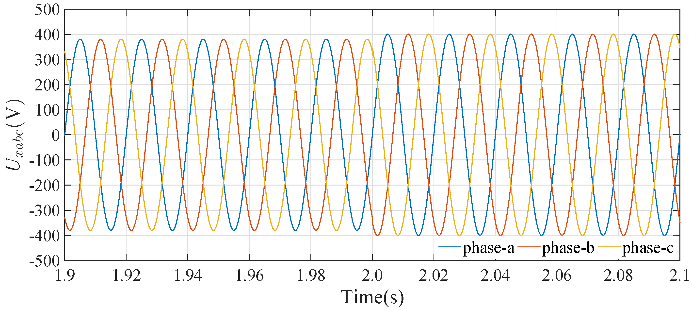
4. Simulation Results

In this section, two detailed types of load (a balanced linear load and an unbalanced linear load) are chosen for the islanded DER system to verify the effectiveness of the proposed voltage control scheme. Moreover, the superiority of the proposed control scheme is compared to the traditional PID control method [28] and fractional-order sliding-mode control (FSMC) [13]. Since the balanced load and unbalanced load are 675 V and 210 V, respectively, the corresponding network-side transformer is used to connect each load. The basic parameters of the two different types of load and the corresponding step-down transformer are given in

Table 1. Load Parameters.

Load Types	Characteristics	Transformer
Balanced	three star-connected	$Tr1$
Load	series RL circuits with	4.13/0.675
	$R=155$ m$\mathsf{\Omega }$ and	kVrms
	$L=200\mathsf{\mu }$H
Unbalanced	series RL between each phase	$Tr2$
Load	and neutral with	4.13/0.21
	$R_a=65$ m$\mathsf{\Omega }$, $L_a=43\mathsf{\mu }$H	kVrms
	$R_b=18$ m$\mathsf{\Omega }$, $L_b=22\mathsf{\mu }$H
	$R_c=25$ m$\mathsf{\Omega }$, $L_c=30\mathsf{\mu }$H

. The detailed parameters of the DER system are shown in

Table 2. The Parameters of the Distributed Energy Resource (DER) System Circuit.

Parameters	Value	Description
$L_s$	$295\mathsf{\mu }$H
C	$500\mathsf{\mu }$F
R	$3.2$ m$\mathsf{\Omega }$
$U_{dc}$	1800 V	dc-link voltage
w	314 rad/s	nominal angular frequency
$Tr$	4.13/ 0.675 kVrms	leakage reactance $8\%$

.

As for the proposed control scheme, we choose the initial values of the estimated PPD parameter matrix $\widehat{\mathsf{\Phi }}(k)$ as ${\widehat{\varphi }}_1(1)=\left[\begin{array}{cc}1.9999& 0.00754\\ -1.00754& 0.9999\end{array}\right]$, ${\widehat{\varphi }}_2(1)=\left[\begin{array}{cc}6200& 5500\\ 5000& 6000\end{array}\right]$, ${\widehat{\varphi }}_3(1)=\left[\begin{array}{cc}-65& 0.0377\\ -55& -0.0677\end{array}\right]$, ${\widehat{\varphi }}_4(1)=\left[\begin{array}{cc}-0.025& -0.02\\ -0.02& -0.03\end{array}\right]$, ${\widehat{\varphi }}_5(1)=\left[\begin{array}{cc}7.54& -0.2\\ -7.54& -0.25\end{array}\right]$.

Other parameter settings of the proposed control algorithm are $\mathbf{K}=diag(0.85,0.85)$, ${\nu }_1={\nu }_2=2\times {10}^4$, $\sigma =diag(0.05,0.45)$. Furthermore, the rate constraints of control input $\mathbf{ø}(k)$ are

$$\begin{array}{c}\hfill \left[\begin{array}{c}-1\hfill \\ -1\hfill \end{array}\right]\le \mathsf{\Delta }\mathbf{ø}(k+1)\le \left[\begin{array}{c}1\hfill \\ 1\hfill \end{array}\right].\end{array}$$

(36)

In the simulation study, $U_{xdref}$ is initially set to 0 while the balanced load is connected to the DER system. At $t=0$ s, the controllers begin to work and the VSC starts receiving gate signals. Then, $U_{xdref}$ is ramped up to 380 V and kept constant from $t=0.5$ s onwards. At $t=1.5$ s, the balanced load is switched off and the unbalanced load is switched on. At $t=2$ s, $U_{xdref}$ is changed stepwise from 380 V to 400 V.

In the simulation of the system, we compared the control effect of the designed MFAC controller with that of the FSMC controller and the traditional PI controller (see in Figure 2). As can be seen from Figure 2, when the reference voltage of the d-axis rises slowly, the d-axis voltage of the DER system under the three control methods begins to track the reference voltage. However, the response of PI controlled system is slow. When $t=0.5$ s, the reference voltage of the d-axis no longer rises and stays at 380 V. At this time, the system response of PI controller is still very slow when the voltage trend changes, and there is a static error between the d-axis voltage controlled by FSMC and the reference voltage. When $t=2$ s, the reference voltage changes from 380 V to 400 V. The d-axis voltage controlled by PI reaches 400 V through 0.05 s, and its change is relatively slow. The d-axis voltage under FSMC control has a small overshoot. Thus, their control effects in the d-axis are not as good as MFAC. Similarly, in the tracking process of q-axis voltage, MFAC control is also superior to the other two control methods. Throughout the whole simulation process, the reference voltage of the q-axis is defined as 0. At the beginning of simulation, the q-axis voltage under FSMC control does not keep up with the reference voltage quickly. When t = 2 s, the q-axis voltage under FSMC control also deviates greatly from the reference voltage. In summary, compared with FSMC and traditional PI control, MFAC has a better control effect during voltage control of the island DER system.

In addition, in Figure 3, Figure 4, Figure 5, Figure 6 and Figure 7, the parameter estimation response curves of ${\varphi }_1(k)$–${\varphi }_5(k)$ are displayed respectively. Figure 8 shows the output voltage waveform at t = 1.9 s–2.1 s. It can be seen that when the reference voltage suddenly changes, the three-phase output voltage of the system changes in time without distortion. Moreover, Figure 2 shows the output current waveform of the system. Compared with Figure 2 and Figure 9, it can be seen that the system voltage under MFAC control remains stable when the current is distorted due to load changes.

5. Conclusions

In this paper, based on the novel transformation and linearization technique for the islanded MIMO DER system dynamics, a multiple observer-based data-driven model free adaptive constrained control scheme was proposed for the voltage control of dispatchable DER system under an unbalanced load condition. Moreover, the proposed control algorithm only depends on the I/O data of the controlled plant and has the advantages of having a small computational burden and strong robustness, which allows easy engineering popularization. In addition, the detailed Lyapunov-based analysis method was presented to guarantee the stability of the closed-loop control system. The simulation model of the DER system was built in MATLAB, and the control effect of MFAC controller was compared with the FSMC and the PI controller, which verifies the advancement of the MFAC controller. In future work, the voltage regulation algorithms for multi-DER systems under the balanced nonlinear load will be the focus of our research.

References

1. Karimi, H.; Nikkhajoei, H.; Iravani, M.R. Control of an electronically-coupled distributed resource unit subsequent to an islanding event. IEEE Trans. Power Deliv. 2008, 23, 493–501. [Google Scholar] [CrossRef]
2. Lew, D.; Asano, M.; Boemer, J.; Ching, C.; Focken, U.; Hydzik, R.; Lange, M.; Motley, A. The power of small: the effects of distributed energy resources on system reliability. IEEE Power Energy Mag. 2017, 15, 50–60. [Google Scholar] [CrossRef]
3. Sajadian, S.; Ahmadi, R. Model Predictive Control of Dual-Mode Operations Z-Source Inverter: Islanded and Grid-Connected. IEEE Trans. Power Electron. 2018, 33, 4488–4497. [Google Scholar] [CrossRef]
4. Chen, Z.; Luo, A.; Wang, H.; Chen, Y.; Li, M.; Huang, Y. Adaptive sliding-mode voltage control for inverter operating in islanded mode in microgrid. Electr. Power Energy Syst. 2015, 66, 133–143. [Google Scholar] [CrossRef]
5. Yazdani, A. Control of an islanded distributed energy resource unit with load-compensating feed-forward. In Proceedings of the IEEE Power and Energy Society General Meeting, PES08, Pittsburgh, PA, USA, 20–24 July 2008. [Google Scholar] [CrossRef]
6. Karimi, H.; Nikkhajoei, H.; Iravani, R. A linear quadratic gaussian controller for a stand-alone distributed resource unit-simulation case studies. In Proceedings of the IEEE Power Engineering Society General Meeting, PES07, Tampa, FL, USA, 24–28 June 2007. [Google Scholar] [CrossRef]
7. Li, Y.; Vilathgamuwa, D.M.; Loh, P.C. Design, analysis, and real-time testing of a controller for multibus microgrid system. IEEE Trans. Power Electron. 2004, 19, 1195–1204. [Google Scholar] [CrossRef]
8. Sao, C.K.; Lehn, P.W. Control and power management of converter fed microgrid. IEEE Trans. Power Syst. 2008, 3, 1088–1098. [Google Scholar] [CrossRef]
9. Delghavi, M.B.; Yazdani, A. Islanded-mode control of electronically coupled distributed-resource units under unbalanced and nonlinear load conditions. IEEE Trans. Power Deliv. 2011, 26, 661–673. [Google Scholar] [CrossRef]
10. Huerta, H.; Loukianov, A.; Canedo, J. Multimachine power-system control: integral-SM approach. IEEE Trans. Ind. Electron. 2009, 56, 2229–2236. [Google Scholar] [CrossRef]
11. Loukianov, A.; Canedo, J.; Utkin, V.; Cabrera-Vazquez, J. Discontinuous controller for power systems: sliding-mode block control approach. Trans. Ind. Electron. 2004, 51, 340–353. [Google Scholar] [CrossRef]
12. Vargas, J.; Ledwich, G. Variable structure control for power systems stabilization. Electr. Power Energy Syst. 2010, 32, 101–107. [Google Scholar] [CrossRef]
13. Delghavi, M.B.; Shoja-Majidabad, S.; Yazdani, A. Fractional-Order Sliding-Mode Control of Islanded Distributed Energy Resource Systems. IEEE Trans. Sustain. Energy 2016, 7, 1482–1491. [Google Scholar] [CrossRef]
14. Chang, F.; Chang, E.; Liang, T.; Chen, J. Digital-signal-processor-based DC/AC inverter with integral-compensation terminal sliding-mode control. IET Power Electron. 2011, 4, 159–167. [Google Scholar] [CrossRef]
15. Su, X.; Han, M.; Guerrero, J.M.; Sun, H. Microgrid stability controller based on adaptive robust total SMC. Energies 2015, 8, 1784–1801. [Google Scholar] [CrossRef] [Green Version]
16. Hou, Z.; Jin, S. A novel data-driven control approach for a class of discrete-time nonlinear systems. IEEE Trans. Control Syst. Technol. 2011, 19, 1549–1558. [Google Scholar] [CrossRef]
17. Hou, Z.; Jin, S. Data driven model-free adaptive control for a class of MIMO nonlinear discrete-time systems. IEEE Trans. Neural Netw. 2011, 22, 2173–2188. [Google Scholar] [CrossRef] [PubMed]
18. Hou, Z.; Wang, Z. From model-based control to data-driven control: survey, classification and perspective. Inf. Sci. 2013, 235, 3–35. [Google Scholar] [CrossRef]
19. Xu, D.; Jiang, B.; Shi, P. A novel model free adaptive control design for multivariable industrial processes. IEEE Trans. Ind. Electron. 2014, 61, 6391–6398. [Google Scholar] [CrossRef]
20. Zhang, H.; Zhou, J.; Sun, Q.; Guerrero, J.M.; Ma, D. Data-Driven Control for Interlinked AC/DC Microgrids Via Model-Free Adaptive Control and Dual-Droop Control. IEEE Trans. Smart Grid 2017, 8, 557–571. [Google Scholar] [CrossRef]
21. Xu, D.; Jiang, B.; Shi, P. Adaptive observer based data-driven control for nonlinear discrete-time processes. IEEE Trans. Autom. Sci. Eng. 2014, 11, 1037–1045. [Google Scholar] [CrossRef]
22. Zhu, Y.; Hou, Z. Data-Driven MFAC for a Class of Discrete-Time Nonlinear Systems With RBFNN. IEEE Trans. Neural Netw. Learn. Syst. 2014, 25, 1013–1020. [Google Scholar] [CrossRef] [PubMed]
23. Zhao, Y.; Yuan, Z.; Lu, C.; Zhang, G.; Li, X.; Chen, Y. Improved model-free adaptive wide-area coordination damping controller for multiple-input-multiple-output power systems. IET Gener. Transm. Distrib. 2016, 10, 3264–3275. [Google Scholar] [CrossRef]
24. Bu, X.; Hou, Z.; Liang, J.; Xu, P. Data driven multiagent systems consensus tracking using model free adaptive control. In Proceedings of the 2016 28th Chinese Control and Decision Conference (CCDC), Yinchuan, China, 28–30 May 2016. [Google Scholar] [CrossRef]
25. Lu, X.P.; Li, W.; Lin, Y.G. Load control of wind turbine based on model-free adaptive controller. Trans. Chin. Soc. Agric. Mach. 2011, 42, 109–114. [Google Scholar]
26. Gao, B.; Gu, K.Y.; Zeng, Y.; Chang, Y. An anti-suction control for an intra-aorta pump using blood assistant index: a numerical simulation. Artif. Organs 2012, 36, 275–285. [Google Scholar] [CrossRef] [PubMed]
27. Spooner, J.; Maggiore, M.; Passino, K. Stable Adaptive Control and Estimation for Nonlinear Systems; Wiley Interscience: Hoboken, NJ, USA, 2002; Volume 36, pp. 275–285. ISBN 0471415464. [Google Scholar] [CrossRef]
28. Astrom, K.; Johansson, K.; Wang, Q. Design of decoupled PI controllers for two-by-two systems. IEE Proc. Control Theory Appl. 2002, 149, 74–81. [Google Scholar] [CrossRef] [Green Version]
Figure 1. Schematic diagram of an islanded DER system.
Energies 11 03299 g001
Figure 2. The tracking effect on the reference voltage.
Energies 11 03299 g002
Figure 3. Parameter estimation response curve of ϕ 1 ( k ) .
Energies 11 03299 g003
Figure 4. Parameter estimation response curve of ϕ 2 ( k ) .
Energies 11 03299 g004
Figure 5. Parameter estimation response curve of ϕ 3 ( k ) .
Energies 11 03299 g005
Figure 6. Parameter estimation response curve of ϕ 4 ( k ) .
Energies 11 03299 g006
Figure 7. Parameter estimation response curve of ϕ 5 ( k ) .
Energies 11 03299 g007
Figure 8. Waveforms of U x a b c under the unbalanced load condition when the proposed control scheme is employed.
Energies 11 03299 g008
Figure 9. Waveforms of I x a b c under the unbalanced load condition when the proposed control scheme is employed.
Energies 11 03299 g009