Icing Degree Characterization of Insulators Based on the Equivalent Collision Coefficient of Standard Rotating Conductors

Abstract

Due to the complex structure of insulators, it is difficult to use parameters such as icicle length or ice thickness of an insulator to directly characterize the degree of icing of an insulator. Rotating conductors are widely used in monitoring icing degree on insulators, but the relationship between ice degree on the insulator and the rotating conductor has not been verified. In this paper, the water droplets collision coefficient α₁ was put forward to characterize icing degree, and a new numerical calculation model where α₁ on different regions of an insulator is calculated was proposed. Combining the freezing fraction α₃ of the insulator and rotating conductor, the equivalent relationship of ice weight between insulator and rotating conductor can be established, which was afterwards verified through the icing tests. The test results indicate that ice weight on an insulator increases linearly with the increase of ice weight on the rotating conductor, and the model proposed in this paper can reflect actual results more accurately than previous models. In such cases, the method of using ice weight on a rotating conductor to predict that on an insulator based on the model proposed in this paper could be widely adopted.

1. Introduction

Since the 20th century, icing and pollution problems have been a threat to the safety and stability of transmission lines, especially icing problems [1,2]. Icing can greatly reduce the mechanical and electrical properties of transmission lines, and thus threaten the power system operation [3]. When insulators are coated with ice, the electrical performance of insulators will drop sharply and it may cause icing flashover which would lead to power supply interruptions [4,5,6,7,8].

Plenty of studies on insulator icing have been carried out by scholars, and they used different ways to characterize the degree of icing. In [9,10], icing weight was proposed to characterize the degree of icing. In [11,12], researchers proposed to gauge the ice thickness of a rotating cylinder in the same environment to represent the degree of icing. Currently, the method of using ice thickness on a standard rotating conductor to characterize the degree of icing of insulators is commonly accepted [13,14]. However, the asymmetry of icing on the surface of an insulator leads to a large measurement error, hence, the existing methods still fail to reflect the actual degree of icing of insulators.

In fluid mechanics, ice accumulation on a structure is caused by the impingements of super-cooled water droplets. These liquid-water droplets freeze immediately upon impact due to rapid heat dissipation [15,16], so icing weight on the structure can be affected by the collision coefficient and the freezing fraction of water droplets. Further, Maeno et al. [17] concluded that freezing fraction can be calculated as a function of environmental temperature, air speed, cylinder diameter and water droplet diameter.

Since the freezing fraction can be calculated using the icing energy-transfer equation, changes of environmental conditions would be directly reflected by the numerical value of water collision coefficient (the ratio of the number of particles colliding on structure to the number of particles contained in the projected area of structure) [18]. Farzaneh et al. [19] used several cylinders of different diameters in place of insulators to simplify the complex calculation of the 3-D flow field outside the insulator. On this basis, Irving et al. [20] calculated the cylinder collision coefficient to analyze pollution model of insulator, and concluded that the total amount of pollution deposited on the entire surface of the insulator is equal to the total amount of pollution particles deposited on the surface of each 2-D cylinder. So far, most studies related to the calculation of collision coefficients are based on an overall calculation model where the collision area of the insulator is considered as a whole [19]. Considering the influences of airflow on windward and leeward of an insulator are different, the water droplet collision coefficient results of insulators are inaccurate.

The work described in this paper was focused on proposing a new model where the equivalent relationship between the ice weight on an insulator and a standard rotating conductor can be more accurately determined. The paper is divided into three parts. To accurately estimate the water droplets collision coefficient on insulators and rotating conductors, a new numerical calculation model is proposed in Section 2, where the collision coefficient of water droplets on different regions of an insulator is calculated. The results estimated by the proposed model are presented in Section 3, while the experimental validation of the calculated results is discussed in Section 4.

2. Numerical Calculation of Water Droplets Collision Coefficient

In this paper, the water droplets collision coefficient (denoted as α₁) is proposed to characterize the degree of icing of insulators and rotating conductors, and the ice weight relationship between an insulator and a rotating conductor can be obtained from the water droplets collision coefficient and freezing fraction calculation results. ANSYS FLUENT (ANSYS Fluent 15.0, ANSYS, Pittsburgh, PA, USA), a CFD software, is used to obtain the field information for the air and water flow field and the volume fraction, which can be used in the proposed icing model to estimate the water droplets collision coefficients on insulators and rotating conductors.

2.1. Definition of the Water Droplets Collision Coefficient

There are two main processes in the process of icing, one is that the water droplets flow and collide with the insulator surface and are trapped by the insulator in a certain proportion, which is described as collision efficiency α₁, and the second one is a freezing thermodynamics process of water film on the insulator, described as α₃.

In this paper, differences of water droplets collision coefficient on different regions of insulator are considered, and two-phase flow is calculated by Lagrange method. As a consequence, α₁ on different regions of insulator can be obtained according to Equation (1):

$${\alpha }_1=\frac{N_{collied}}{N_{\mathrm{total}}}=\frac{N_{collide}}{S_{0}n}$$

(1)

where, N_collide is the number of water droplets colliding on different regions of insulator; N_total is the number of water droplets contained in the projected area of insulator in the direction of flow; S₀ is the projected area of the cross section of the insulator in the direction of flow; n is the number of water droplets per unit area of water droplets released.

2.2. Establishment and Mesh Generation of Numerical Geometry Model of Water Droplets Collision Coefficient

Figure 1 shows the profile of the XP-70 insulator (XP-70, Dalian Insulator Group Co., Dalian, Liaoning Province, China), with a shed diameter of 254 mm, shed height of 146 mm, leakage distance of 295 mm, which was selected as the experimental test specimen.

Due to the complex structure of the XP-70, it is difficult to calculate the water droplets collision rate within each microelement of the insulator surface. In a previous study, to calculate either the water droplets collision coefficient [21] or particle collision coefficient [22] on the insulator surface, the collision area was analyzed as a whole. There are no studies which analyze the differences of collision coefficient in different regions of insulator. Consequently, it is impossible to reflect differences in different regions of insulator during the icing process, but in practice, in addition to the significant differences between the windward side and the leeward side of insulator icing, icing on different positions of the windward side of insulator is also uneven. Results in [21] show that there is more ice on the rod and the edge of shed of composite insulator than on the middle of the shed on the windward side.

In order to improve the accuracy of the analysis, this paper proposes a new model where the cases of water droplets colliding with different regions of the insulator are analyzed, respectively. Considering the difficulty of calculation and differences of water droplets collision coefficients in different regions of insulators, this paper proposes to divide the surface of the XP-70 into four parts including: ① windward cap, ② windward shed, ③ windward edge of shed and ④ leeward, as shown in Figure 2.

Due to the XP-70’s complex structure and irregular surface, it is not convenient to model it directly in ANSYS ICEM (ANSYS ICEM 15.0, ANSYS, Pittsburgh, PA, USA). In this paper, a 3-D parameterized solid model of the insulator was established firstly in AutoCAD (AutoCAD 2007, Autodesk, San Rafael, CA, USA), then the computing domain was established and the mesh was generated in ANSYS ICEM, as shown in Figure 3. In establishing the computing domain, the calculation area is divided into two parts, namely, the near wall area and far wall area. In dividing the grid, a tetrahedral mesh was used in mesh generation of the near wall area and hexahedral and prismatic meshes were used in the mesh generation of the far wall area.

A standard rotating conductor with a diameter of 28 mm and a height of 600 mm is chosen as the study object in this paper. For the methods of the establishing computing domain and generating the mesh one can refer to those of the insulator. The mesh generation of the rotating conductor is shown in Figure 4.

2.3. The Determination of Boundary Conditions of the Numerical Calculation of Water Droplets Collision Coefficients

In this paper, a one-way coupling calculation method was obtained in simulating the gas-liquid two-phase flow field outside the insulator. First, the airflow was solved independently. Then the trajectory of water droplets was simulated by using the particle orbital model in a Lagrangian coordinate system. Turbulent flow was set to standard k-ε turbulence model [23] to fix the RANS (Reynold average Nevier-Stokes) control equation. The standard near-wall function was selected as the wall function. The governing equations were selected in the QUICK (Quadratic Upwind Interpolation for Convection Kinetics scheme) format. The Semi-Implicit Method for Pressure Linked Equation (SIMPLE) algorithm was selected in solving the discrete equations and the standard format was applied in the pressure interpolation.

In solving the continuous flow field, the turbulence intensity I and turbulence scale L could be obtained based on the empirical equations I = 0.16(R_e) − 0.125 (R_e is the number of Reynolds) and L = 0.07 l (l is the hydraulic diameter of the wind tunnel). The export was set as the boundary condition of the outflow. Water droplets were set to launch from the inlet boundary, and the velocity was set as same as that of the airflow. In the calculations, this paper assumed that water droplets freeze immediately on the insulator and ice on insulator has no effect on the trajectory of water droplets. Water droplets which have been trapped by the wall and escape from the export were no longer tracked. Consequently, the insulator wall was set in trap mode, and other walls were set in escape mode.

3. Results and Analysis of Numerical Simulation of Water Droplets Collision Coefficient

In this paper, the trajectory of the water droplets and external flow field outside insulator and rotating conductor were simulated in different environments. Because changes of temperature have no effect on α₁, temperature conditions are no longer considered here [24].

3.1. Results and Analysis of Numerical Simulation of Water Droplets Collision Coefficient on Rotating Conductor

In Fluent, α₁ under different wind velocity (denoted as U) and median volume diameter (denoted as MVD) conditions was simulated. After the calculation, it is possible to obtain the air relative velocity vector, as shown in Figure 5.

As shown in Figure 5, the rotating conductor displays a strong disturbance in the airflow around it. Airflow on the windward side is stronger than that on the leeward side. Because the diameter of water droplets is small, their movement would be greatly influenced by the airflow. Consequently, there are more water droplets colliding with the rotating conductor on the windward side than on the leeward side. Based on [25], the freezing fraction α₃ is same on the windward side and the leeward side of a rotating conductor. In such cases, the ice weight on the rotating conductor on the windward side is more than that on the leeward side of the rotating conductor.

Because the rotating conductor rotates along its axis at a constant angular speed, the overall probability of water droplets colliding on the surface of the rotating conductor is equivalent. In consequence, ice on the rotating conductor is uniform.

When MVD is regarded as a single variable, α₁ increases with an increase of MVD under different wind velocity U, as shown in Figure 6.

Figure 6 presents the following:

(i)

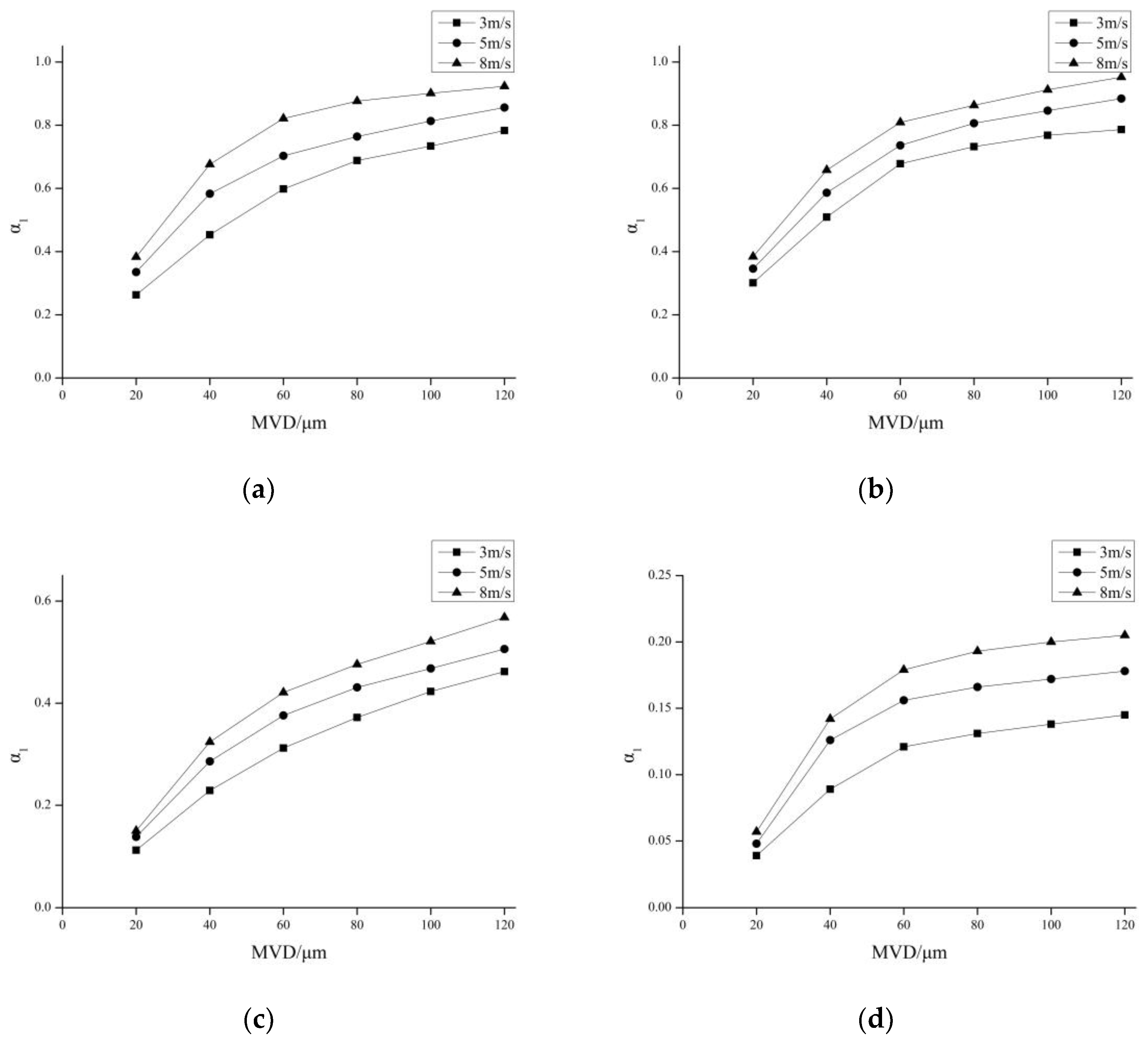
When the wind velocity U or MVD increases and the other remains constant, it will lead to an increase of α₁.

(ii)

The change regularities of α₁ on the rotating conductor under different U appear to be similar. However, the increase trend of α₁ slows down gradually with an increase of MVD from 20 μm to 120 μm. This can be explained as follows: with an increase of diameter, water droplets have a weaker following character with the airstream. In such cases, droplets have greater possibilities of maintaining their original trajectories, resulting in a slower increase of α₁. Under the same wind velocity, small droplets are more susceptible to airflow than large ones.

3.2. Results and Analysis of Numerical Simulation of Water Droplets Collision Coefficient on Insulator

In Fluent, α₁ under different wind velocity (denoted as U) and median volume diameter (denoted as MVD) was simulated. Based on calculation results simulated by Fluent, it is possible to obtain the air relative velocity vector, as shown in Figure 7.

As is shown in Figure 7, air flows from the edge of shed to the cap on the windward side, and the intensity of airflow gradually decays from the shed to the cap. As mentioned above, the movement of water droplets would be greatly influenced by the airflow. Consequently, the number of water droplets colliding with the insulator on the windward side decreases with a decrease of airflow. After airflow bypasses the cap and shed of insulator, the airflow velocity changes greatly, and can be divided into two areas. The velocity of airflow near the cap is smaller than that near the shed on the leeward side of the insulator. This can be explained as follows: without a direct disturbance like the cap, airflow near the shed on the leeward side does not change as much as that near the cap on the leeward side. Consequently, this will result in the fact that there are fewer water droplets colliding with the surface of insulator on the windward side than on the leeward side. Based on [25], the freezing fraction on the insulator on the windward and leeward side are same, so the ice weight on the windward side of the insulator is more than that on the leeward side.

When MVD is regarded as a single variable, α₁ based on the model proposed in this paper increases with an increase of MVD under different wind velocity U, as shown in Figure 8, which presents the following:

(i)

When the wind velocity U or MVD increases and the other remains constant, it will lead to an increase of α₁.

(ii)

α₁ is different on different regions of the insulator. The numbers of water droplets trapped by the edge of shed and the cap of insulator on the windward side are similar, and both of them are much larger than that of the shed on windward side. Besides, α₁ on the shed is almost 2–3 times that on the insulator surface on the leeward side.

(iii)

The change regularities of α₁ on the windward cap, windward edge of the shed and leeward appear to be similar, but one essential difference can be identified, that is, unlike other regions of the insulator, the change regularity of α₁ on the windward shed of the insulator is approximately a straight line.

4. Characterization and Verification of Insulator Icing Degree Based on the Equivalent Collision Coefficient

4.1. Characterization of Insulator Icing Degree Based on the Equivalent Collision Coefficient

Experts and scholars at home and abroad have conducted voluminous research on ice weight on the surface of a cylinder [26]. According to [18,27], icing weight occurring on a cylinder in $\Delta t$ can be calculated by:

$$\Delta m={\alpha }_1·{\alpha }_3·w·U·D·L·\Delta t$$

(2)

where, α₁ is the water droplets collision coefficient, α₃ is the freezing fraction, w (g/m³) is the liquid water content, U (m/s) is the inflow velocity, D (m) is the diameter of the icing cylinder, L (m) is the height of the icing cylinder; $\Delta t$ is a tiny time interval. Because the insulator’s shed has a certain dip angle, water droplets cannot collide with the lower surface of insulator directly. In this paper, the underside of the insulator surface is not considered, and hence the insulator surface is equivalent to the lateral surface of the cylinder and circular frustum. As is shown in Figure 2, parts ① ③ ④ are equivalent to the cylinder, and ② is equivalent to the lateral surface of the cylinder. The height of the equivalent cylinder is as same as the original structure, and the diameter of the cylinder can be calculated by:

$$D=\frac{S}{\pi h}$$

(3)

where, S (m²) is the lateral area of the circular frustum or cylinder, h (m) is the height of the circular frustum or cylinder. In such cases, parameters such as α₁, w, U, D, L could be determined already. According to [28], the freezing fraction α₃ can be calculated by theoretical Equation (4):

$$\begin{array}{ll}{\alpha }_3=& \frac{\pi h(T_{\mathrm{s}}-T)+\frac{0.62\pi h{L}_e}{c_{a}p}[e(T_s)-e(T)]}{{\alpha }_{1}wU[L_f+c_i(273.15-T_s)+c_w(T_s-T)]}\\ & +\frac{4\pi \epsilon {\sigma }_R{T}^3(T_s-T)}{{\alpha }_{1}wU[L_f+c_i(273.15-T_s)+c_w(T_s-T)]}\\ & +\frac{c_w(T_s-T)+c_w(273.15-T)-\frac{h{r}_{c}U}{2c_a{\alpha }_{1}w}-\frac{U^2}{2}}{L_f+c_i(273.15-T_s)+c_w(T_s-T)}\end{array}$$

(4)

$$Where, e(T)=0.61121\exp (\frac{18.678-\frac{T}{234.5}}{257.14+T}\times T); N_u=C·{R_e}^n·{P_r}^{\raisebox{1ex}{$1$}\!\left/ \!\raisebox{-1ex}{$3$}\right.}; h=\frac{k_a·N_a}{D_i}; R_e=(D+2d_i)·U/v; P_r=v/a$$

(5)

where, h (J/m²·K) is the convective heat transfer coefficient; T (K) is the environmental temperature; T_s (K) is the temperature of the structure surface on the dynamic balance of icing; L_e (L_e = 2.51 × 10⁶ J/kg) is the potential of evaporation or sublimation at T_s; c_i (c_i = 2090 J/kg·°C) is the specific heat of ice; c_a (c_a = 1014 J/kg·K) is the specific heat of air; w (g/m³) is the liquid water content; U (m/s) is the inflow velocity; L_f (L_f = 3.35 × 10⁵ J/kg) is the melting potential of ice; c_w (c_w = 4.2 × 10³ J/kg·K) is the specific heat of water; r_c (r_c = 0.79) is the recovery coefficient of local viscous heating on the surface of the rotating conductor; k_a (k_a = 0.0244 W/m·°C) is the heat transfer coefficient of air; D_i (m) is the cylinder diameter after icing; σ_R (σ_R = 5.5670 × 10⁻⁸ W/m²·K⁴) is the Stefan-Boltzman constant; D (m) is the diameter of the rotating icing conductor; d_i (m) is the icing thickness; v (v = 1.328 × 10⁻⁵ m²/s) is dynamic viscosity of air; a (a = 1.88× 10⁻⁵ m²/s) is the thermal diffusivity of air; N_u is the Nusselt number; C (C = 0.683) and n (n = 466) are constants in icing; R_e is the Reynolds number; P_r is the Prandtl number.

Combining the partition method of the XP-70 in the model proposed in this paper and the shed configuration shown in Figure 2, the icing weight accumulated on the cap, the shed, the edge of shed and the leeward of XP-70 insulator can be expressed as m₁, m₂, m₃, m₄, respectively.

The theoretical ice weight on the insulator m_d can be obtained through Equation (6):

$$m_{\mathrm{d}}=m_1+m_2+m_3+m_4$$

(6)

where, m_d (g) is the ice weight on the insulator, m₁ (g) is the ice weight on the cap on the windward side, m₂ (g) is the ice weight on the shed on the windward side, m₃ (g) is the ice weight on the edge of the shed on the windward side, m₄ (g) is the leeward ice weight.

This paper defines k₁ as theoretical ratio of insulator ice weight to rotating conductor ice weight:

$$k_1=m_{\mathrm{d}}/m_{\mathrm{eq}}$$

(7)

where, m_d (g) is the ice weight on the insulator, m_eq (g) is the ice weight on the rotating conductor.

Similarly, through using α₁ based on model in [19] and Equation (2), another theoretical ice weight m_d where the collision area is considered as a whole can be obtained. Results of k₁ based on the model proposed in this paper and in [19] under different U, T and MVD are shown in

Table 1. Theoretical ratio k₁ of insulator ice weight to rotating conductor ice weight.

MVD (μm)	U (m/s)	T (°C)	k1
			In This Paper	Model in [19]
20	3	−2	4.487	7.364
	5	−2	2.329	3.213
	8	−2	1.598	1.788
40	3	−2	2.356	2.78
	5	−2	1.505	1.235
	8	−2	1.039	0.804
60	3	−2	2.059	2.07
	5	−2	1.328	1.007
	8	−2	0.84	0.666
80	3	−2	1.794	1.732
	5	−2	1.203	0.92
	8	−2	0.722	0.576
100	3	−2	1.658	1.558
	5	−2	1.127	0.869
	8	−2	0.684	0.549
	3	−6	2.571	4.559
	5	−6	1.873	2.547
	8	−6	1.419	1.611
	3	−10	2.809	4.895
	5	−10	2.289	3.821
	8	−10	1.956	2.561
120	3	−2	1.531	1.401
	5	−2	1.044	0.809
	8	−2	0.649	0.523

.

4.2. Test Verification and Analysis

This paper defines k₁ as theoretical ratio of insulator ice weight to rotating conductor ice weight. All the experimental investigations in this paper were conducted in a multifunction artificial climate chamber with a diameter of 7.8 m and a height of 11.6 m, shown in Figure 9 The minimum temperature in the chamber could be adjusted to −45 ± 1 °C. The wind velocity varies between 3 m/s and 5 m/s, and its atomizing nozzle can control MVD between 15 and 200 μm, which meets the requirements in [29].

The experiments were divided into two parts, the first part was conducted by changing the wind velocity while the other one changed the environmental temperature. In each icing experiment, the icing time was set within 1 h, and the icing weight was measured every twenty minutes.

As is shown in Figure 10 (first experimental condition: T is −6 °C, MVD is 100 μm, w is 1.1 g/m³) and Figure 11 (second experimental condition: T is −2 °C, U is 3 m/s, MVD is 100 μm, w is 1.1 g/m³. third experimental condition: T is −10 °C, U is 3 m/s, MVD is 100 μm, w is 1.1 g/m³), ice on the windward side of the insulator is much more than that on the leeward side, and ice on the cap of the insulator on the windward side is more than that on the shed on the windward side. This result corresponds to the analysis provided above. Due to the uniform rotation of the rotating conductor during icing, ice on the rotating conductor is uniform.

Results of icing weight on the insulator and rotating conductor are shown in

Table 2. Ice weight of insulator and rotating conductor (first experimental condition).

Ice Structure	U/m/s	Ice Weight/g
		20 min	40 min	60 min
XP-70	3	151	316	480
	5	178	365	546
Rotating conductor	3	65	140	198
	5	82	176	259

,

Table 3. Ice weight of insulator and rotating conductor (second experimental condition).

Ice Structure	U/m/s	Ice Weight/g
		20 min	40 min	60 min
XP-70	3	19	51	80
Rotating conductor	3	11	30	44

and

Table 4. Ice weight of insulator and rotating conductor (third experimental condition).

Ice Structure	U/m/s	Ice Weight/g
		20 min	40 min	60 min
XP-70	3	176	380	580
Rotating conductor	3	69	147	220

.

Based on the test results in Table 2, Table 3 and Table 4, the corresponding relationship of ice weight between the XP-70 insulator and a rotating conductor in different environmental conditions can be obtained, as shown in Figure 12.

As is shown in Figure 12, ice weight on the insulator increases with a liner increase of ice weight on the rotating conductor, and k is defined as the ratio of ice weight on the insulator to ice weight on the rotating conductor to represent this:

$$k=\frac{m_c}{m_s}$$

(8)

where, m_c (g) is the experimental ice weight on the insulator, m_s (g) is the experimental ice weight on the rotating conductor.

In this paper, σ₁ is defined as the relative error between the experimental value k and the theoretical value k₁. Results of k₁, k and σ₁ under different conditions are shown in

Table 5. The theoretical and testing ratio of insulator ice weight to rotating conductor ice weight.

MVD (μm)	U (m/s)	T (°C)	k	k1		σ1 (%)
				In This Paper	Model in [19]	In This Paper	Model in [19]
20	3	−2	1.66	1.78	1.56	7.23	6.14
	3	−6	2.57	2.36	4.56	8.17	77.4
	5	−6	1.87	2.10	2.55	12.3	36.2
	3	−10	2.81	2.62	4.90	6.76	74.2

.

$${\sigma }_1=\frac{\left|k_1-k\right|}{k}\times 100\%$$

(9)

Table 5 presents the following:

(i)

The change trends of both the theoretical ratio k₁ based on the model proposed in this paper and in [19] are in agreement with the experimental ratio k. With an increase of U and T, the ratio of ice weight on the insulator to ice weight on the rotating conductor decreases.

(ii)

The relative error σ₁ based on the model proposed in this paper is much smaller than that based on the model proposed in [19]. Comparing with the model proposed in [19], the calculation used in the model proposed in this paper takes the influence of different shapes and diameters in different regions into account, and calculates α₁ and α₃ in different regions respectively. In such cases, the calculation results based on the model proposed in the paper are more accurate than those of the model proposed in [19].

(iii)

The relative error σ₁ based on the model proposed in this paper between the ratio k₁ and k is less than 15%. Simulation results obtained using the model proposed in this paper are consistent with the experimental results. In test verification, the equivalence of ice weight between insulator and rotating conductor has been established. Hence, if other parameters like wind velocity U, environmental temperature T, α₃, LWC (liquid water content) et al. are determined, α₁ can be used as the parameter to characterize the ice weight of insulators and rotating conductors.

5. Conclusions

This study explores the relationship of ice weight on an insulator and a rotating conductor through simulation in Fluent and test verification in an artificial climate chamber. The main conclusions are as follows:

(i)

Using Fluent to simulate the icing process of an insulator and a rotating conductor, the simulation results show that when any one of the wind velocity and MVD increases and other environmental parameters remain constant, it would lead to an increase of α₁.

(ii)

The experimental verification indicates that ice weight on insulator increases with a liner increase of ice weight on rotating conductor, and k (defined as the ratio of ice weight on insulator to ice weight on rotating conductor) decreases with a decrease of either MVD or U.

(iii)

Compared with the results calculated by the model proposed in [19], the results calculated by the model proposed in this paper are closer to the test results. In such case, the calculation results calculated by the model proposed in this paper are more accurate than those proposed in [19].

(iv)

In this paper, the equivalent relationship of ice weight between the insulator and rotating conductor is established. Therefore, the method of using ice weight on a rotating conductor to predict that on an insulator based on the model proposed in this paper can be widely adopted.

References

- Oikonomou, D.S.; Maris, T.I.; Ekonomou, L. Artificial intelligence assessment of sea salt contamination of medium voltage insulators. In Proceedings of the 8th WSEAS International Conference on Systems Theory and Scientific Computation (ISTASC’ 08), Rhodes, Greece, 20–22 August 2008; pp. 319–323. [Google Scholar]
- Pappas, S.S.; Ekonomou, L. Comparison of adaptive techniques for the prediction of the equivalent salt deposit density of medium voltage insulators. WSEAS Trans. Power Syst. 2017, 12, 220–224. [Google Scholar]
- Farzaneh, M. Insulator flashover under icing conditions. IEEE Trans. Dielectr. Electr. Insul. 2014, 21, 1997–2011. [Google Scholar] [CrossRef]
- Jiang, X.; Xiang, Z.; Zhang, Z.; Hu, J.; Hu, Q.; Shu, L. Predictive Model for Equivalent Ice Thickness Load on Overhead Transmission Lines Based on Measured Insulator String Deviations. IEEE Trans. Power Deliv. 2014, 29, 1659–1665. [Google Scholar] [CrossRef]
- Hu, Q.; Wang, S.; Shu, L.; Jiang, X.; Liang, J.; Qiu, G. Comparison of Ac Icing Flashover Performances of 220 kV Composite Insulators with Different Shed Configurations. IEEE Trans. Dielectr. Electr. Insul. 2016, 23, 995–1004. [Google Scholar] [CrossRef]
- Hu, Q.; Yuan, W.; Shu, L.; Jiang, X.; Wang, S. Effects of Electric Field Distribution on Icing and Flashover Performance of 220 kV Composite Insulators. IEEE Trans. Dielectr. Electr. Insul. 2014, 21, 2181–2189. [Google Scholar]
- Li, Z.; Zhang, Q.; Liu, F.; Jia, H.; Cheng, L.; Xi, H. Discharge propagation along the air gap on an ice-covered insulator string. IEEE T. Plasma Sci. 2011, 39, 2238–2239. [Google Scholar] [CrossRef]
- Emran, S.M.A.; Farzaneh, M. Flashover Performance of Ice-Covered Post Insulators with Booster Sheds Using Experiments and Partial Arc Modeling. IEEE Trans. Dielectr. Electr. Insul. 2016, 23, 979–986. [Google Scholar] [CrossRef]
- Hu, J.; Sun, C.; Jiang, X.; Shu, L. Flashover performance of pre-contaminated and ice-covered composite insulators to be used in 1000 kV UHV AC transmission lines. IEEE Trans. Dielectr. Electr. Insul. 2007, 14, 1347–1356. [Google Scholar] [CrossRef]
- Jiang, X.; Wang, Q.; Zhang, Z.; Hu, J.; Qin, H.; Yang, P.; Yi, C.; Jiang, X.; Wang, Q.; Zhang, Z. Estimation of Rime Icing Weight on Composite Insulator and Analysis of Shed Configuration. IET Gener. Transm. Distrib. 2018, 12, 650–660. [Google Scholar]
- Farzeneh, M.; Kiernicki, J. AC flashover performance of insulators covered with artificial ice. IEEE Trans. Power Deliv. 1995, 10, 123–127. [Google Scholar] [CrossRef]
- Farzaneh, M.; Baker, T.; Brown, K.; Chisholm, W. Insulator icing test methods and procedure. IEEE Power Eng. Rev. 2007, 22, 64. [Google Scholar] [CrossRef]
- Fu, P.; Farzaneh, M.; Bouchard, G. Two-dimensional modeling of the ice accretion process on transmission line wires and conductors. Cold Reg. Sci. Technol. 2006, 46, 132–146. [Google Scholar] [CrossRef]
- Farzaneh, M.; Kiernicki, J. Flashover performance of IEEE standard insulators under ice conditions. IEEE Trans. Power Deliv. 1997, 12, 1602–1613. [Google Scholar] [CrossRef]
- Langmuir, I.; Blodgett, K. A mathematical investigation of water droplet trajectories. Collect. Works Irving Langmuir 1946, 10, 348–393. [Google Scholar]
- Maeno, N.; Makkonen, L.; Nishimura, K.; Kosugi, K. Growth rates of icicles. J. Glaciol. 1994, 40, 319–326. [Google Scholar] [CrossRef] [Green Version]
- Fu, P.; Farzaneh, M. A CFD approach for modeling the rime-ice accretion process on a horizontal-axis wind turbine. J. Wind Eng. Ind. Aerodyn. 2010, 98, 181–188. [Google Scholar] [CrossRef]
- Farzaneh, M. Atmospheric Icing of Power Networks; Springer: Quebec, QC, Canada, 2008. [Google Scholar]
- Ravelomanantsoa, N.; Farzaneh, M.; Chisholm, W.A. Insulator pollution processes under winter conditions. In Proceedings of the 2005 Annual Report Conference on Electrical Insulation and Dielectric Phenomena, Nashville, TN, USA, 16–19 October 2005; pp. 321–324. [Google Scholar]
- Irving, L.; Blodgett, K. Mathematical Investigation of Water Droplet Trajectories; Army Air Force Technology: Washington, DC, USA, 1946. [Google Scholar]
- Horenstein, M.N.; Melcher, J.R. Particle contamination of high voltage DC insulators below corona threshold. IEEE Trans. Electr. Insul. 1979, 14, 297–305. [Google Scholar] [CrossRef]
- Fu, P. Modelling and Simulation of the Ice Accretion Process on Fixed or Rotating Cylindrical Objects by the Boundary Element Method. Ph.D. Thesis, University of Quebec in Chicoutimi, Chicoutimi, QC, Canada, 2004. [Google Scholar]
- Yeuan, J.J.; Liang, T.; Hamed, A. Viscous simulations in a transonic fan using k-ε and algebraic turbulence models. In Proceedings of the 36th Aerospace Sciences. Meeting & Exhibit, Reno, NV, USA, 12–15 January 1998; Volume 932. [Google Scholar]
- Jiang, X.; Han, X.; Hu, Y.; Yang, Z.; Jiang, X.; Han, X.; Hu, Y.; Yang, Z.; Jiang, X.; Han, X. A Model for Ice Wet Growth on Composite Insulator and Its Experimental Validation. IET Gener. Transm. Distrib. 2018, 12, 556–563. [Google Scholar] [CrossRef]
- Myers, T.G.; Charpin, J.P.F.; Thompson, C.P. Slowly accreting ice due to supercooled water impacting on a cold surface. Phys. Fluids 2002, 14, 240–256. [Google Scholar] [CrossRef]
- Makkonen, L. Models for the growth of rime, glaze, icicles and wet snow on structures. Philos. Trans. A Math. Phys. Eng. Sci. 2000, 358, 2913–2939. [Google Scholar] [CrossRef]
- Makkonen, L. Modeling of ice accretion on wires. J. Clim. Appl. Meteorol. 1984, 23, 929–939. [Google Scholar] [CrossRef]
- Chao, Y. Study on the Model and Impact Factors of Boundled Conductors and Parallel Composite Insulator Strings Icing. Ph.D. Thesis, Chongqing University, Chongqing, China, 2011. [Google Scholar]
- Draft Guide for Test Methods and Procedures to Evaluate the Electrical Performance of Insulators in Freezing Conditions; IEEE: Piscataway, NJ, USA, 2009.