1. Introduction
Icing on transmission lines might lead to ice flashovers of insulators, collapse of towers, tripping faults of transmission lines, and other accidents [
1]. The main reasons for ice flashover include: the electrolyte of pollution from air and insulator surface increasing freezing-water capacity; the ice bridging between two adjacent insulators sheds leading to decline of icing flashover voltage [
2,
3,
4].
Insulator surface pollution is the main reason for flashover occuring in distribution lines. It can also be affected by multiple factors including temperature, humidity, wind velocity, rain and fog, property and quantity of pollution sources, insulator configuration (represented by equivalent salt deposit density (ESDD)), leakage current, and surface pollution layer capacity (SPLC) [
5,
6,
7]. In recent years, there have been many methods to assess the contamination of insulators based on artificial neural networks (ANN) [
5], multi model partitioning filter (MMPF) [
6], etc. Also, insulator icing flashover is affected by meteorological conditions, including ice type and structure [
7]. However, there are no appropriate methods to denote and assess icing conditions between insulator sheds.
With the development of computer graphics, scholars have started to research insulator condition monitoring based on video or image processing [
7,
8]. Image processing of icing transmission lines has been researched widely due to its regular configuration. Chongqing University analyzed transmission line and insulator surface icing images based on edge extraction methods [
9]. Xi’an Polytechnic University applied image matching to transmission line galloping monitoring using image gray processing, image enhancement method, and image segmentation [
10]. Some scholars have researched equivalent icing thickness representation for transmission lines based on LOG operator edge detection, wavelet multi-scale analysis, and Hough conversion [
11,
12,
13].
The graphical processing method of icing insulators has recently gained attention. Dalian Maritime University proposed a segmentation method of aerial insulator based on principal component analysis and an active contour model [
14,
15]. The Chinese Academy of Sciences detected insulators in video sequences using tilt correction, feature extraction, and a support vector machine (SVM) [
16]. North China Electric Power University extracted insulator margins from aerial photos using a non-subsampled contourlet transform (NSCT) [
17].
Ice morph is complex and fickle [
18], which adds difficulty in research to recognize icing degree by image processing. Xi’an Polytechnic University proposed to segment insulators from images before and after icing, and estimate icing degree by comparing insulator contour before and after icing. Nevertheless, this was not verified by experiment [
19]. Chongqing University proposed a method to monitor insulator’s icing by calculating the volume difference before and after icing based on three-dimensional reconstruction and then calculating ice mass according to rime density (0.5 g/cm
3) [
20,
21]. However, it is hard to install cameras and power on-site; three-dimensional reconstruction needs at least three cameras. The method used for calculating icing thickness on transmission lines was not applicable for insulators due to their complex structure.
In this paper, the GrabCut segmentation algorithm is proposed to segment ice-covered insulators from images. Compared with the other four image processing methods, the results of GrabCut are superior in terms of contour smoothness and accuracy. For analyzing insulator icing conditions quantitatively, we define and make use of two effective parameters (i.e., graphical shed overhang and graphical shed spacing) to recognize convexity defect of ice-covered insulator string contour. The axial and the radial icing bridge degrees between insulator sheds are denoted by the change of graphical shed spacing and graphical shed overhang. Using image data from our climatic chamber and the China Southern Power Grid Disaster (Icing) Warning System of Transmission Lines, graphical shed spacing and graphical shed overhang are comparatively investigated as a new evaluation method for glass insulator icing conditions.
2. Theory and Method
As the contours of insulator string are convex graphical shed spacing (D) and graphical shed overhang (P) are calculated by recognizing convexity defect of insulator contours after GrabCut-based segmentation.
2.1. Image Segmentation by GrabCut
2.1.1. Maximum Flow and Minimum Cut
The key of GrabCut image segmentation is to determine the graphical maximum flow and minimum cut under maximum flow.
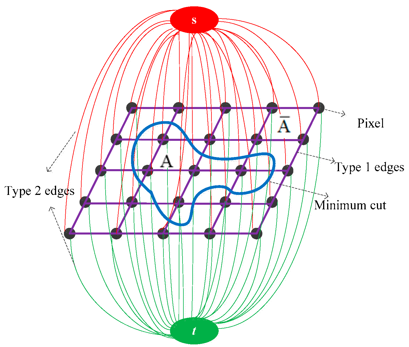
Firstly, an image is mapped to a capacity network where each graphical pixel corresponds to a node. In addition, there are two extra nodes, a source node (
s) and a sink node (
t).
s represents the foreground (or research object) and
t represents background (i.e., the image except for the research object), as shown in
Figure 1.
There are two types of edges: (1) the edges that link adjacent pixels and (2) the edges that link pixels to
s or
t.
Um,n, the capacity of type 1 edges, represents the capacity between adjacent pixels
m and
n;
Un,s and
Un,t, the capacity of type 2 edges, respectively represent the capacity between pixel
n and
s or
n and
t. The capacity of type 1 edges denotes a difference between adjacent pixels, and the capacity of type 2 edges denotes the probability that a pixel belongs to the foreground or background. For example, if a pixel belongs to foreground, the capacity (the probability that it belongs to foreground) between the pixel and
s is the maximum value, and the capacity (the probability that it belongs to background) between the pixel and
t is 0. If the pixel belongs to background for certain, the capacity between the pixel and
s is 0, and the capacity between the pixel and
t is the maximum value. If a pixel does not belong to the foreground or the background, the capacity between the pixel and
s or
t is between 0 and the maximum value. The calculations of
Um,n,
Un,s, and
Un,t are detailed in
Section 2.1.2.
If
P is the full set, to a set
A, existing
,
, then
is a cut set or “cut” of the network, and
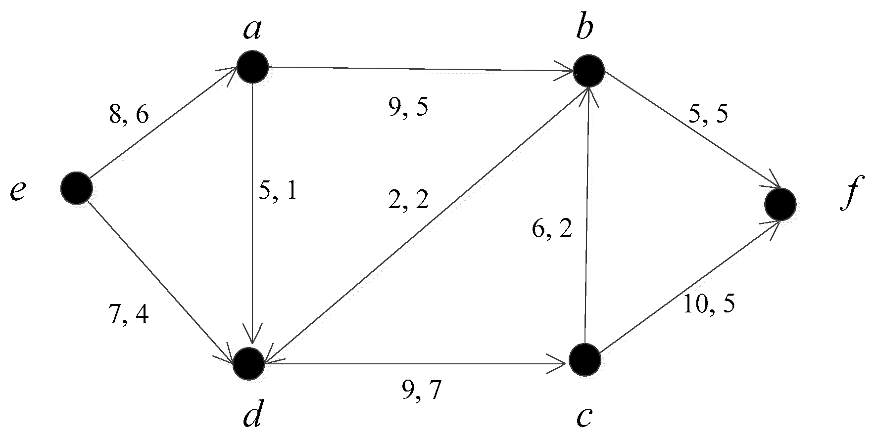
is the cut magnitude. An
A directed flow network is shown in
Figure 2, where the flow of edges describes the amount of capacity that is in use. In
Figure 2, the first number on each edge represents the capacity and the second represents the current flow. If
,
, and
is a cut of the network, and the cut magnitude = 7 + 5 + 2 + 5 = 19.
In any network, the maximum flow corresponds to the cut magnitude under the minimum cut. In
Figure 1, the minimum cut corresponds to the maximum flow from
s, through pixels, to
t. The deduction and calculation for maximum flow and minimum cuts in maximum flow is detailed in literature [
22].
If the minimum cut of
is shown as the blue closed curve in
Figure 2 using maximum flow algorithm,
A consists of all nodes in the blue closed curve and the source
s, while
consists of all nodes that are beyond the blue closed curve and the sink
t. The pixel points could be segmented to the foreground or background according to the minimum cut.
2.1.2. Calculation Method of Um,n, Un,s, and Un,t
The formula to calculate
Um,n, the capacity of type 1 edges, is shown in Equation (1) [
22]
where
zm and
zn, respectively, denote color grey level of pixel m and
n,
β denotes the priority of type 1 edges over type 2 edges,
C represents a pair of neighboring pixels, and the exponential coefficient is used to adapt the contrast degree of the image.
β can magnify this difference when the contrast degree of the image is low, which is shown in
where
denotes the sum of all neighboring pixel pairs in the image, and
N denotes the number of
m and
n pairs.
The calculation of Un,s and Un,t (i.e., the capacity of type 2 edges) is described as follows.
If n is determined as part of the foreground, Un,s is assigned as L (take L = 9γ, with the definition of γ identical to that in Equation (1)) and Un,t as 0. If n is determined as part of the background, Un,s is assigned as 0 and Un,t as L.
Otherwise, if
n cannot be determined as part of the background or foreground,
Un,s and
Un,t is determined by a Gaussian mixture model. Assume that the Gaussian mixture model is shown through Equations (3) and (4).
where
and 0 ≤
w ≤ 1,
K is the element number of the Gaussian mixture model, which is 3 in this paper.
a can be
s or
t, if a is assigned as
s,
Gs represents the Gaussian mixture model of the foreground; if
a is assigned as
t,
Gt represents the Gaussian mixture model of the background;
wa,j represents the weights of the
ith Gaussian model
g(
zn;
μa,I,
σa,i);
zn represents the pixel to be segmented, where
μa,i and
σa,i, respectively, represent the mean value and covariance matrix of the
ith Gaussian model.
The calculation of
Un,s and
Un,t are respectively shown as Equations (5) and (6) [
23]
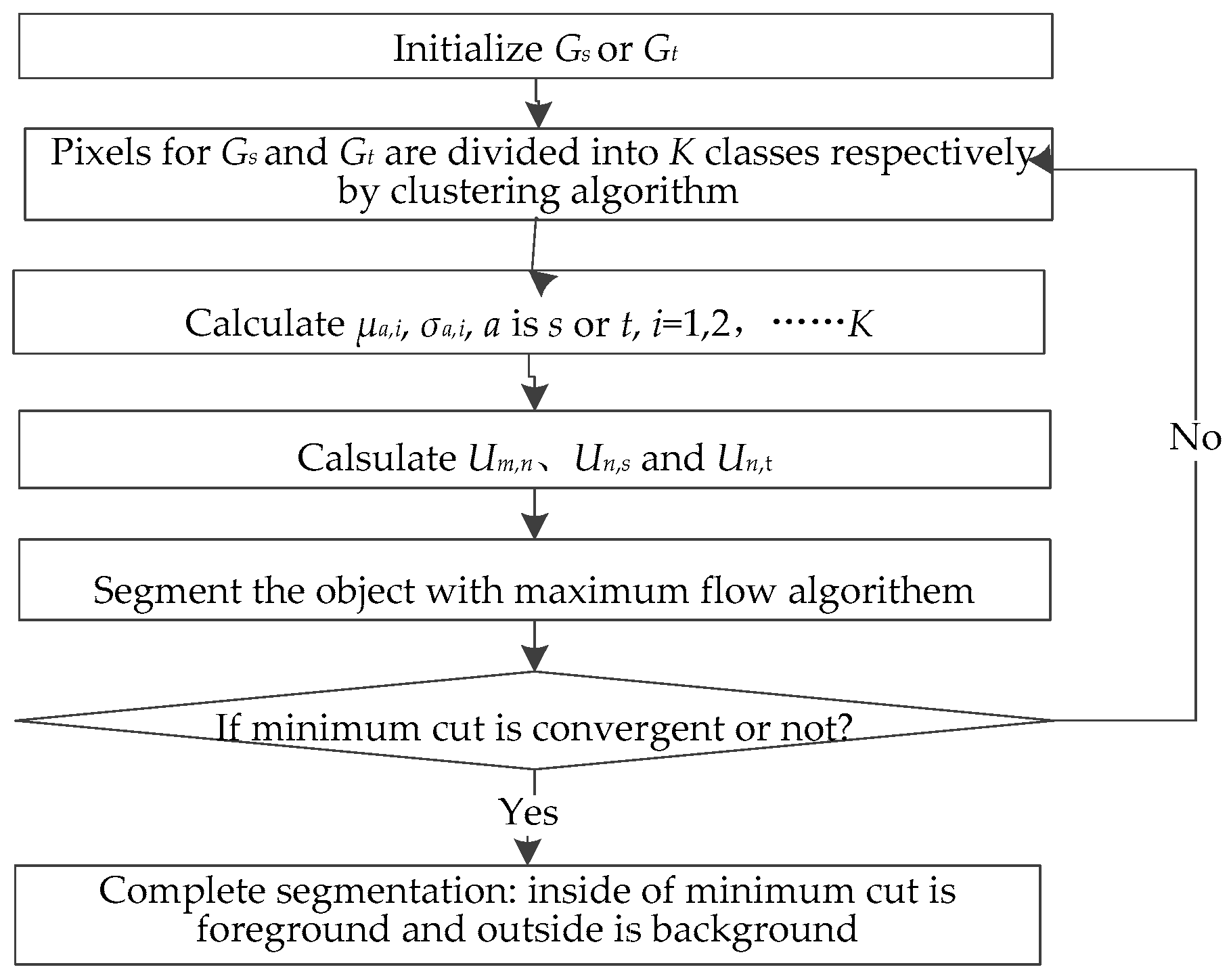
2.1.3. GrabCut Segmentation Algorithm
This paper analyzes the images of transmission line glass insulators using the GrabCut segmentation algorithm, whose flowchart is shown as
Figure 3.
First,
Gs or
Gt is initialized according to selected rectangle in images; the pixels inside the rectangle are for
Gs, and pixels outside the rectangle are for
Gt. Next, pixels for
Gs and
Gt are divided into
K classes respectively using a clustering algorithm based on the color grey value. The
Gs or
Gt belongs to the
ith Gaussian model. This paper uses a K-means [
23] clustering algorithm, and
K is equal to 3. Next, the parameters for mean value (
μa,i) and covariance matrix (
σa,i) are calculated for each element in Gaussian mixture model according to color grey value of pixels in each class.
Then, the parameters
zm,
zn,
μa,i, and
σa,i are put into Equations (1), (5), and (6). The capacities of the two edge types (i.e.,
Um,n,
Un,s, and
Un,t) are calculated. Finally, the object is segmented using the maximum flow algorithm described in
Section 2.1.1.
This is repeated from the clustering algorithm until the minimum cut is convergent.
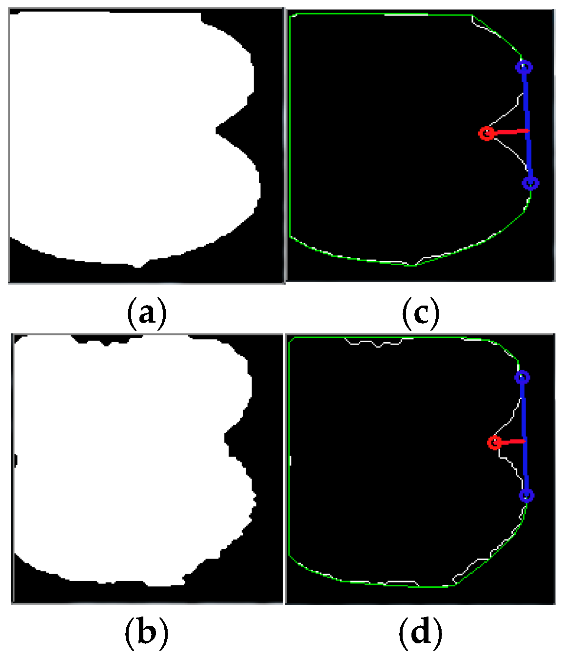
2.2. Convex Hull and Convexity Defect
The contour of the insulator string from images before icing could be seen as a concave polygon, and its concavity would decrease with ice accretion. The contour may even become a convex polygon with severe ice accretion. Therefore, the contour of the insulator string from images may reflect the icing situation of insulators.
The convex hull of a concave polygon refers to its minimum enclosing convex polygon, and the convexity defect of a concave polygon refers to the complementary part for the concave polygon to be convex [
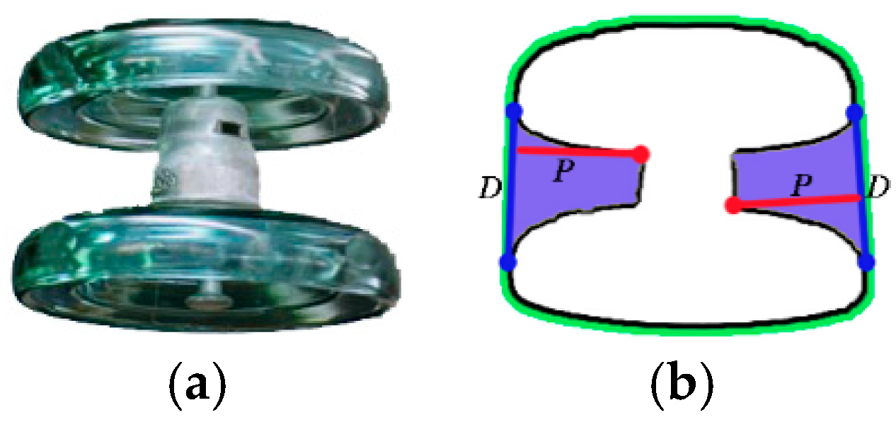
24]. For example, the contour, convex hull, and convexity defect of two adjacent glass insulator sheds in
Figure 4a are shown as
Figure 4b, the black line indicates contour, the green line indicates the convex hull and the purple region indicates the convexity defect.
There are three important parameters for a convexity defect: starting point, ending point, and depth. As shown in
Figure 4b, the starting point and ending point are intersection points of convex hull and convexity defect, which are marked with blue points. The deepest point of a convexity defect is one with maximum vertical distance from contours of insulator to convex hull, which is marked with a red point. The depth of a convexity defect refers to the vertical distance from the deepest point to the line
D determined by the starting and ending points.
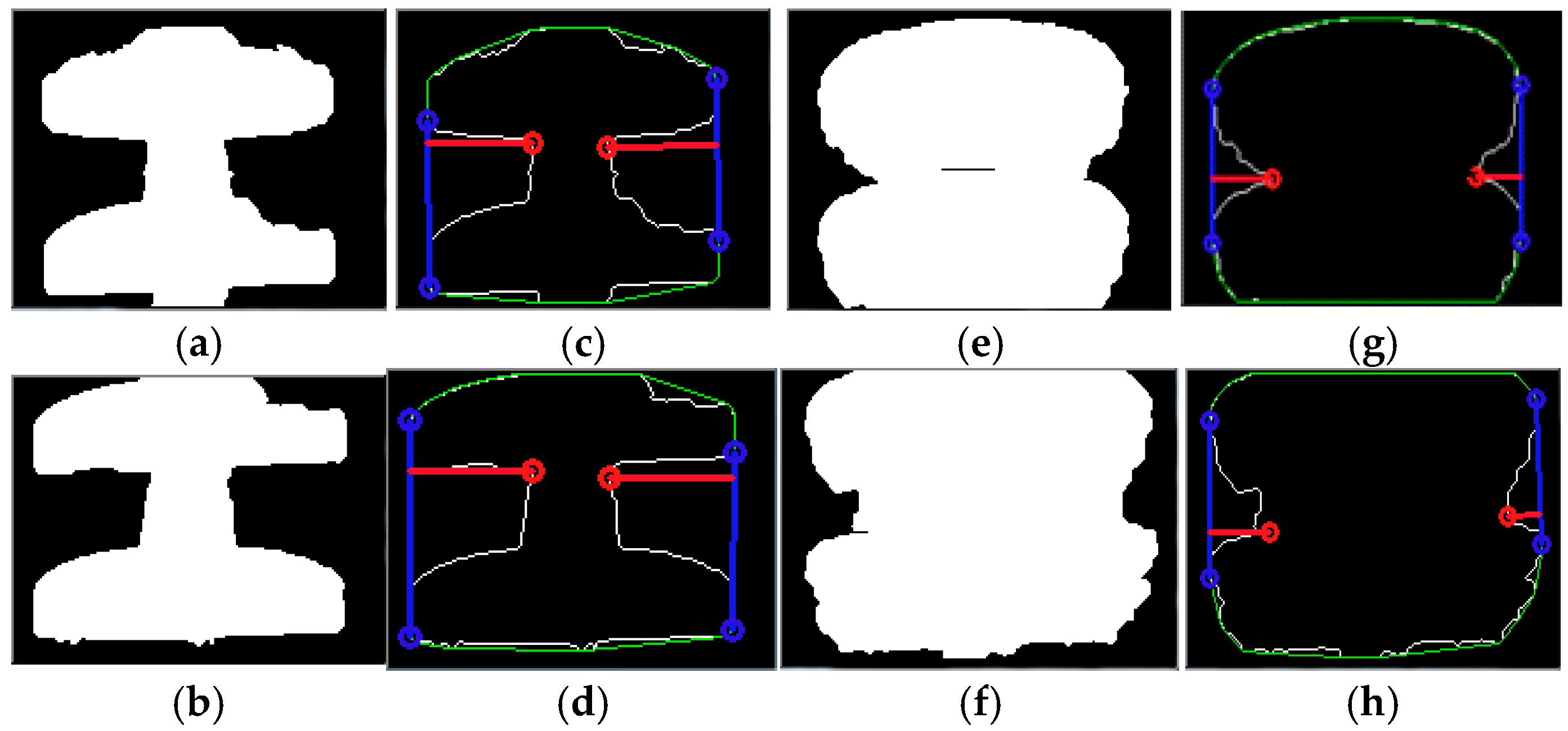
2.3. Computation of Graphical Shed Spacing and Graphical Shed Overhang
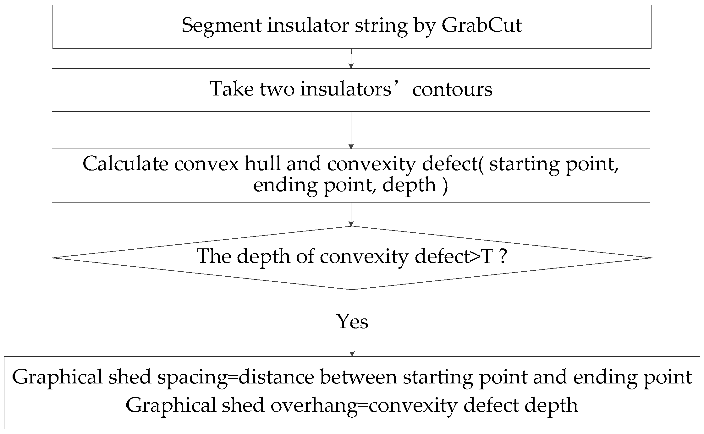
The computation flow chart is shown as
Figure 5. First, the convex hull and convexity defect are calculated. The images of ice-covered and non-ice-covered insulator string are segmented using the GrabCut algorithm, which can take two insulators’ contours. The insulators’ contours are presented as many concaves, and convex hull are consist of pixels belonging to minimum convex set on the contours [
24]. The starting point, ending point, and depth are calculated.
Then, there may be many small concaves on insulator contours, especially in icing conditions because ice forms are irregular. However, only the changes in the concaves between adjacent sheds are a cause for concern. This paper selects convexity defects with depth less than T. The value of T depends on the size of an insulator shed in pixel, which is set to 10 in this paper.
According to the starting point, ending point, and depth, the graphical shed spacing is approximately equal to the distance between the starting point and ending point (D), and the graphical shed overhang is approximately equal to the convexity defect depth (P). The computation results are represented as a distance measured pixels distance.
2.4. Relationship of Graphical Shed Spacing, Graphical Shed Overhang, and Icing Degree
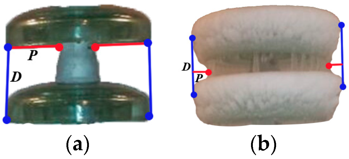
The insulators before and after icing are shown in orthographic in
Figure 6. In
Figure 6b, both the upper and lower surface of insulator sheds are covered with ice and the shed spacing are bridged by icicles. It is deduced that the change of
D and
P may relate to icing degree.
The bridging degree may differ for insulator sheds from the same insulator string. We can estimate icing degree of the whole insulator string according to the average change percent of
D and
P, represented as △
Da (%) and △
Pa (%), respectively, and shown in Equations (7) and (8) below.
where
N denotes the number of insulator sheds.
Dil and
Dir denote respectively the left and the right graphical shed spacing between the
ith and the number (
i + 1)th sheds.
Pil and
Pir respectively denote the left and the right graphical shed overhang between the
ith and the number (
i + 1)th sheds.
Dil′,
Dir′,
Pil′, and
Pir′ denote the related graphical shed spacing and shed overhang after icing.
3. Results and Discussion
In this section, the segmentation results of GrabCut are presented and compared the performance with threshold method [
25], Sobel method, Canny method [
26], and seed region growth method [
27]. Then, to make quantitative analysis of icing conditions, the change of graphical shed overhang and graphical shed spacing are discussed in different icing conditios.
3.1. Image Processing Results and Comparisons
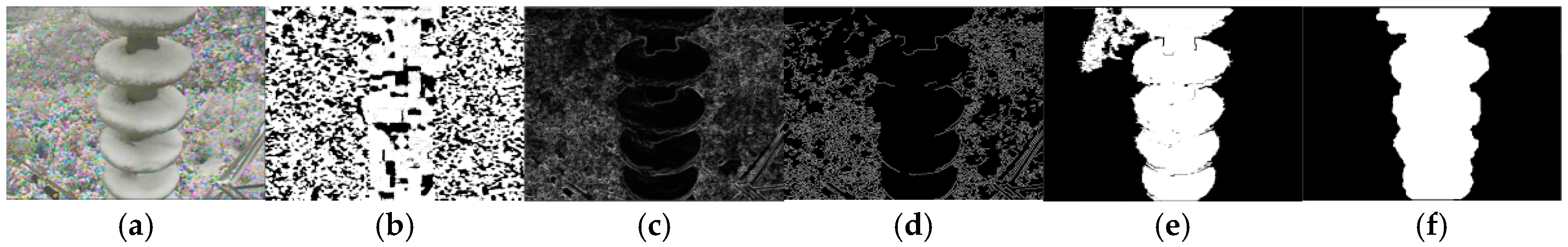
Figure 7 shows the segmentation results in terms of five image processing methods. It is clearly shown that the contours of ice-covered insulator are not segmented properly from background by Threshold method.
Figure 7c,d are the results of Sobel and Canny method based on edge detection algorithm, although better segmentations are obtained, there are still a lot of edges from the background that is not enough to accurately monitor icing conditions.
Figure 7e shows the segmentation results using seed region growth method. However, the contours of ice-covered insulator are irregular and the threshold values have to be set based on various icing conditions [
27]. As shown in
Figure 7f, the segmentation results of GrabCut are superior to the other four methods in terms of the contour smoothness and accuracy.
Based on observing that the contours could be segmented as an enclosing convex polygon using GrabCut, two parameters (i.e., graphical shed overhang and graphical shed spacing) are defined and leveraged using the contour convexity defect recognition. In contrast, the other four methods cannot get graphical shed spacing and graphical shed overhang to analyze icing conditions quantitatively.
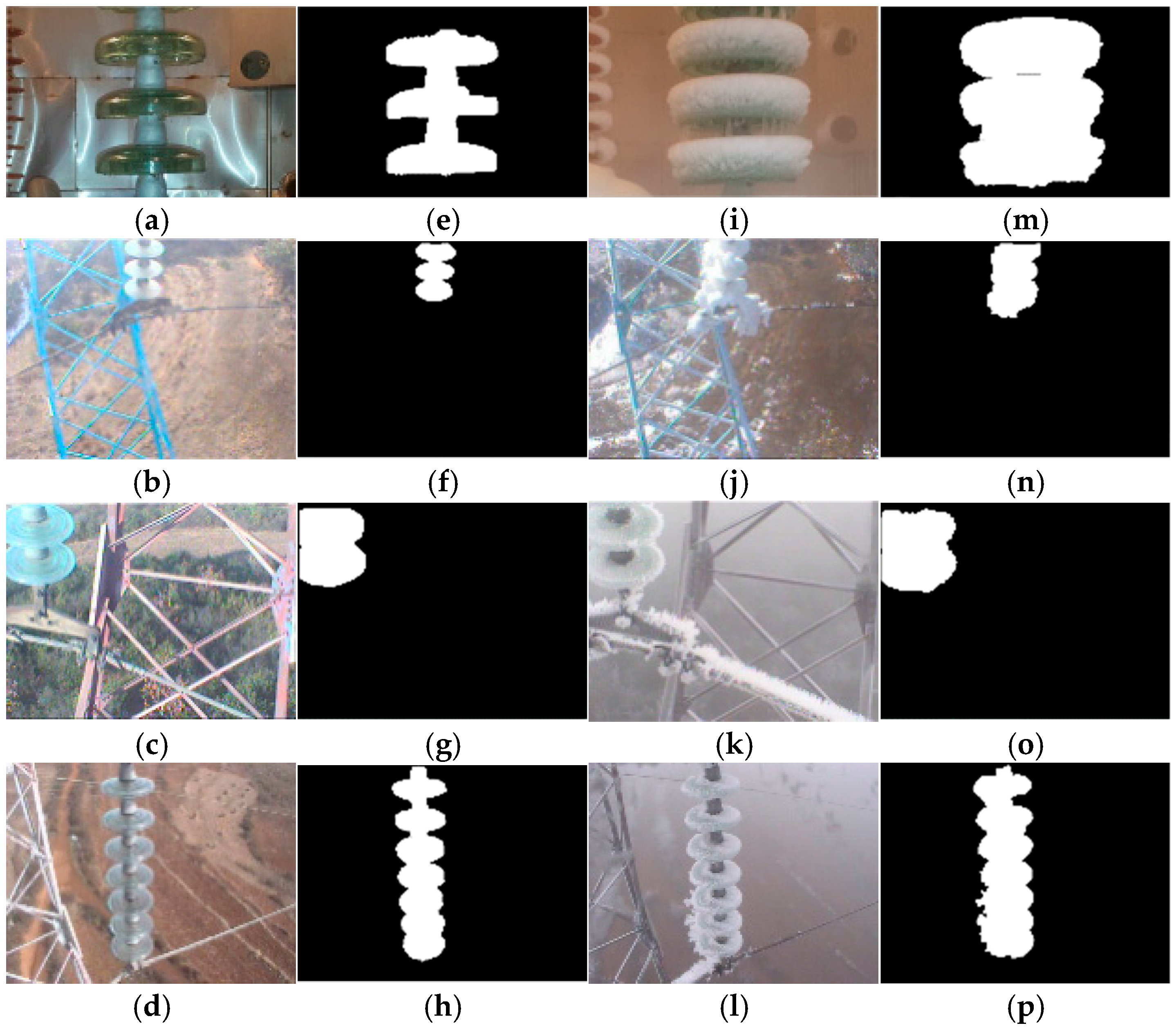
To demonstrate the effectiveness of the method we proposed, the experiments are carried out with image data from our climatic chamber and China Southern Power Grid Disaster (Icing) Warning System of Transmission Lines. By the above analysis, insulator icing conditions of four groups are estimated based on the changes of graphical shed spacing and graphical shed overhang. Group 1 is from our climatic chamber with a humidity of 100% and a water conductivity of 2.5 × 10⁻² S/m, and the other three groups (i.e., Group 2, Group 3, and Group 4) are from China Southern Power Grid Disaster (Icing) Warning System of Transmission Lines. The sizes of these images from these two sources are 375 × 256 and 640 × 480, respectively.
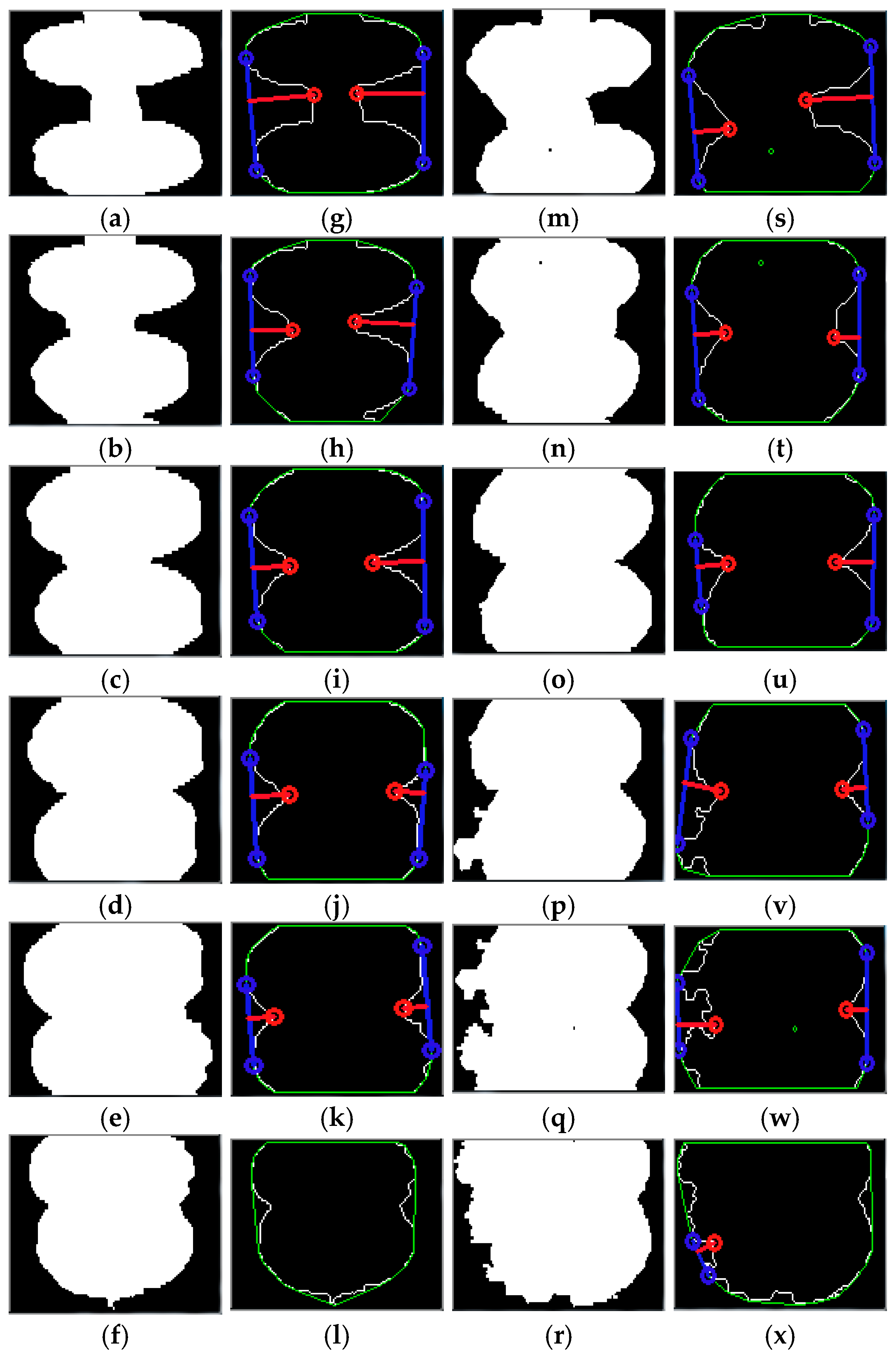
The four groups of insulator images include images without ice and that with ice. Their segmentation results using GrabCut are shown in
Figure 8. There convex hull and convexity defect are shown in
Figure 9,
Figure 10,
Figure 11 and
Figure 12.
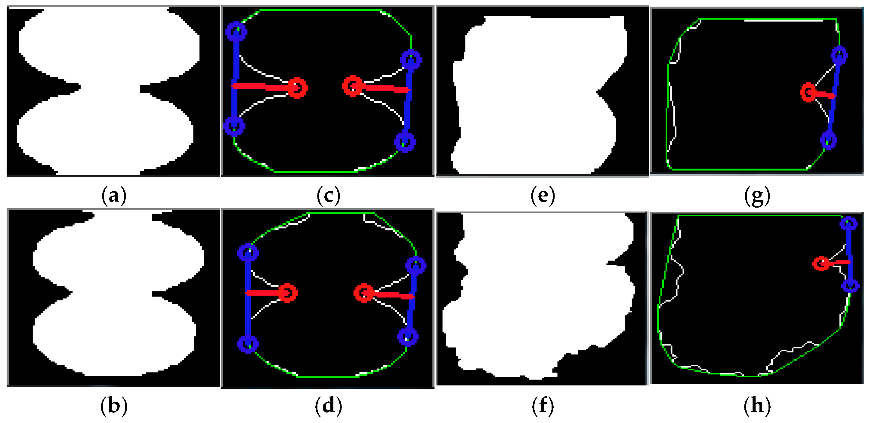
3.2. The Change of Graphical Shed Overhang and Spacing in Different Icing Conditions
Based on the results of insulator convexity defect from
Figure 9,
Figure 10,
Figure 11 and
Figure 12, we get percentage changes of insulator graphical shed spacing after icing, as seen in
Table 1, where
Dl′,
Dr′, and
Da′ represent the left, right, and average graphical shed spacing after icing, respectively. △
Dl (%), △
Dr (%), and △
Da (%) represent change percentage of the left, right, and average graphical shed spacing after icing, respectively. The computation of △
Da (%) is shown as Equation (7), △
Dm (%) denotes the maximum absolute value of change percentage of graphical shed spacing for an insulator string.
From the
Table 1, it is evident that the changes of average graphical shed spacing for insulators with ice is small (|△
Da (%)| < 20%). In Group 2, △
Dl (%) = 0, which indicates that, in the worst icing conditions, sheds are completely bridged in the radial direction. In Group 3, graphical shed spacing and graphical shed overhang cannot be detected due to visual angle.
The change percentages of graphical shed overhang for insulators with ice are shown in
Table 2, where
Pl′,
Pr′, and
Pa′ represent the left, right and average graphical shed overhang after icing, respectively. △
Pl (%), △
Pr (%), and △
Pa (%) represent the change percentage of left, right, and average graphical shed overhang after icing, respectively, and the computation of △
Pa (%) is shown in Equation (8), and △
Pm (%) denotes the maximum absolute value of change percentage of graphical shed overhang for an insulator string.
|△Pa (%)| is much larger than |△Da (%)| in heavy ice. For example, △Da (%) in Group 1, Group 2 and Group 3 are −2.45%, 6.33%, and 1.13%, respectively. However, △Pa (%) of these are −49.77%, −68.32%, and −20%, respectively. In Group 2, graphical shed spacing is completely bridged after icing, where △Pl (%) = −100%. When the number of insulator sheds is much larger, the bridging degree in different positions and directions may differ. It is significant to concern the worst icing conditions. For example, in Group 4, △Pa (%) is −16.47%, while △Pm (%) is −52.5%. However, in Group 4, icing on the bottom three insulator sheds is quite irregular, estimation via change percent of graphical shed overhang after icing has errors.
4. Conclusions
In this paper, graphical shed spacing and graphical shed overhang of in-service glass insulators are proposed to assess insulator icing conditions. This is implemented with GrabCut segmentation and contour convexity defect recognition. The main conclusions are as follows.
The GrabCut segmentation algorithm is proposed to process images of the ice-covered insulator. Compared with the other four image processing methods, the GrabCut algorithm is more superior to extract the contours of the ice-covered insulator from original images. Based on GrabCut segmentation algorithm, graphical shed overhang and graphical shed spacing are calculated using contour convexity defect recognition. The overall icing condition for an insulator string is calculated by average and maximum graphical shed spacing and graphical shed overhang. The results show that the graphical shed overhang of insulators show evident change due to icing. This method can recognize icing conditions quantitatively, e.g., the heavy ice from radial insulator sheds are completely bridged where △Pl (%) = −100%. Also, it can detect bridging position including the left side, the right side, or both sides of the insulator strings in the image.


