In M&V, one often uses the baseline data (
) to infer the baseline (pre-retrofit) model parameters
through an inverse method:
where
is a function relating the independent variables (energy governing factors) to the energy use of the facility, and
is time. The model parameters describe the sensitivity of the energy model to the independent variables such as occupancy, outside air temperature, or production volume.
As an aside, this section will discuss an elementary parametric energy model using Bayesian regression, similar to standard linear regression. In practice, a two-parameter linear regression model seldom captures the different states of a facility’s energy use, for example, heating at low temperatures, a comfortable range, and cooling at high temperatures. Piecewise linear regression techniques are often used [
48,
49,
50,
51,
52], and they tend to work reasonably well if their assumptions are satisfied, but they are not stable in all cases, are approximate, and the assumptions are often restrictive. Shonder and Im [
17] provide a Bayesian alternative. A non-parametric model using a Gaussian Process could also be used, and since one does not need to specify a parametric model, it allows very flexible models to be fit while still quantifying uncertainty. This is especially useful for models where energy use is a nonlinear function of the energy governing factors. However, to keep the example simple and focussed, only a simple parametric model will be considered below.
3.2.1. Example
Suppose one has a simple regression model where the energy use of a building
is correlated with the outside air temperature through the number of Cooling Degree Days (CDD). One cooling degree day is defined as an instance where the average daily temperature is one degree above the thermostat set point for one day, and the building therefore requires one degree of cooling (Technical note: a more accurate description would be the “building balance point”, where the building’s mass and insulation balance external forcings [
53]). Let the intercept coefficient be
, the slope coefficient
, and the Gaussian error term
. One could then write:
In standard linear regression, one would write
as the vector of two coefficients and do some linear algebra to obtain their estimates. There would be a standard error on each, which would indicate their uncertainties, and if the assumptions of linear regression, such as normality of residuals, independence of data, homoscedasticity, etc. hold, then it would be accurate. In Bayesian regression, one would describe the distributions on the parameters:
where
is the vector of the standard deviations on the estimates. Generating random pairs of values from the posterior, at a given value of CDD, according to the appropriate distributions, will yield the posterior predictive distribution. This is the distribution of energy use at a given temperature, or over the range of temperatures. Overlaying such realisations onto the actual data is called the posterior predictive check (PPC).
Now, consider a concrete example. The IPMVP 2012 [
5] (Appendix B-6) contains a simple regression example of creating a baseline of a building’s cooling load. The twelve data points themselves were not given, but a very similar data set yielding almost identical regression characteristics has been engineered and is shown in
Table 1.
A linear regression model was fit to the data, and yielded the result shown in
Table 2.
3.2.3. Bayesian Solution
The key to the Bayesian method is to approach the problem probabilistically, and therefore view all parameters in Equation (
9) as probability distributions, and specify them as such. In this regression model, there are three parameters of interest: the intercept (
), slope (
), and the response (
). This response is the likelihood function, familiar to most readers as the frequentist approach. These distributions need to be specified in the Bayesian model. First, consider the priors on the slope and intercept. These can be vague. Technical note: the uniform prior on
in Equation (
11) is actually technically incorrect: it may seem uniform in terms of gradient but is not uniform when the angle of the slope is considered. It is therefore not “rotationally invariant” and biases the estimate towards higher angles [
54]. The correct prior is
; this is uniform on the slope angle. The reason that Equation (
11) works in this case is that the exponential weight of the likelihood masks the effect. However, this is not always the case, and analysts should be careful of such priors in regression analysis:
and
Now, consider the likelihood. In frequentist statistics, one needs to assume that
in Equation (
9) is normally distributed. In the Bayesian paradigm, one may do so, but it is not necessary. A Student’s
t-distribution is often used instead of a Normal distribution in other statistical calculations (e.g.,
t-tests) due to its additional (“degrees of freedom”) parameter, which accommodates the variance arising from small sample sizes more successfully. As in
Section 3.1.2, an exponential distribution on the degrees of freedom (
) is specified. It has also been found that specifying a Half-Cauchy distribution on the standard deviation (
) works well [
55]. Therefore, the hyperpriors are specified as:
and:
The mean of the likelihood is the final hyperparameter that needs to be specified. This is simply Equation (
9), written with the priors:
The full likelihood can thus be written as:
The PyMC3 code is shown below:
| import pymc3 as pm |
| with pm.Model() as bayesian_regression_model: |
| # Hyperpriors and priors: |
| nu = pm.Exponential(’nu’, lam=1/len(CDD)) |
| sigma = pm.HalfCauchy(’sigma’, beta=1) |
| slope = pm.Uniform(’slope’, lower=0, upper=20) |
| intercept = pm.Uniform(’intercept’, lower=0, upper=10000) |
| # Energy model: |
| regression_eq = intercept + slope*CDD |
| # Likelihood: |
| y = pm.StudentT(’y’, mu=regression_eq, nu=nu, sd=sigma, observed=E) |
| # MCMC calculation: |
| trace = pm.sample(draws=10000, step=pm.NUTS(), njobs=4) |
The last line of the code above invokes the MCMC sampler algorithm to solve the model. In this case, the No U-Turn Sampler (NUTS) [
56] was used, running four traces of 10,000 samples each, simultaneously on a four-core laptop computer, in 3.5 min fewer samples, could also have been used.
A discussion of the inner workings and tests for adequate convergence of the MCMC is beyond the scope of the study and has been done in detail elsewhere in literature [
4]. The key idea for M&V practitioners is that the MCMC, like MC simulation, must converge, and must have done enough iterations after convergence to approximate the posterior distribution numerically. For most simple models such as the ones used in most M&V applications, a few thousand iterations are usually adequate for inference. Two popular checks for posterior validity are the Gelman–Rubin statistic
[
57,
58] and the effective sample size (ESS). The Gelman–Rubin statistic compares the four chains specified in the program above, started at random places, to see if they all converged on the same posterior values. If they did, their ratios should be close to unity. This is easily done in PyMC3 with the
pm.gelman_rubin(trace) command, which indicates
equal to one to beyond the third decimal place. However, even if the MCMC has converged, it does not mean that the chain is long enough to approximate the posterior distribution adequately because the MCMC mechanism produces a serially correlated (autocorrelated) chain. It is therefore necessary to calculate the
effective sample size: the sample size taking autocorrelation into account. In PyMC3, one can invoke the
pm.effective_n(trace) command, which shows that the ESSs for the parameters of interest are well over 1000 each for the current case study. As a first-order approximation, we can therefore be satisfied that the MCMC has yielded satisfactory estimates.
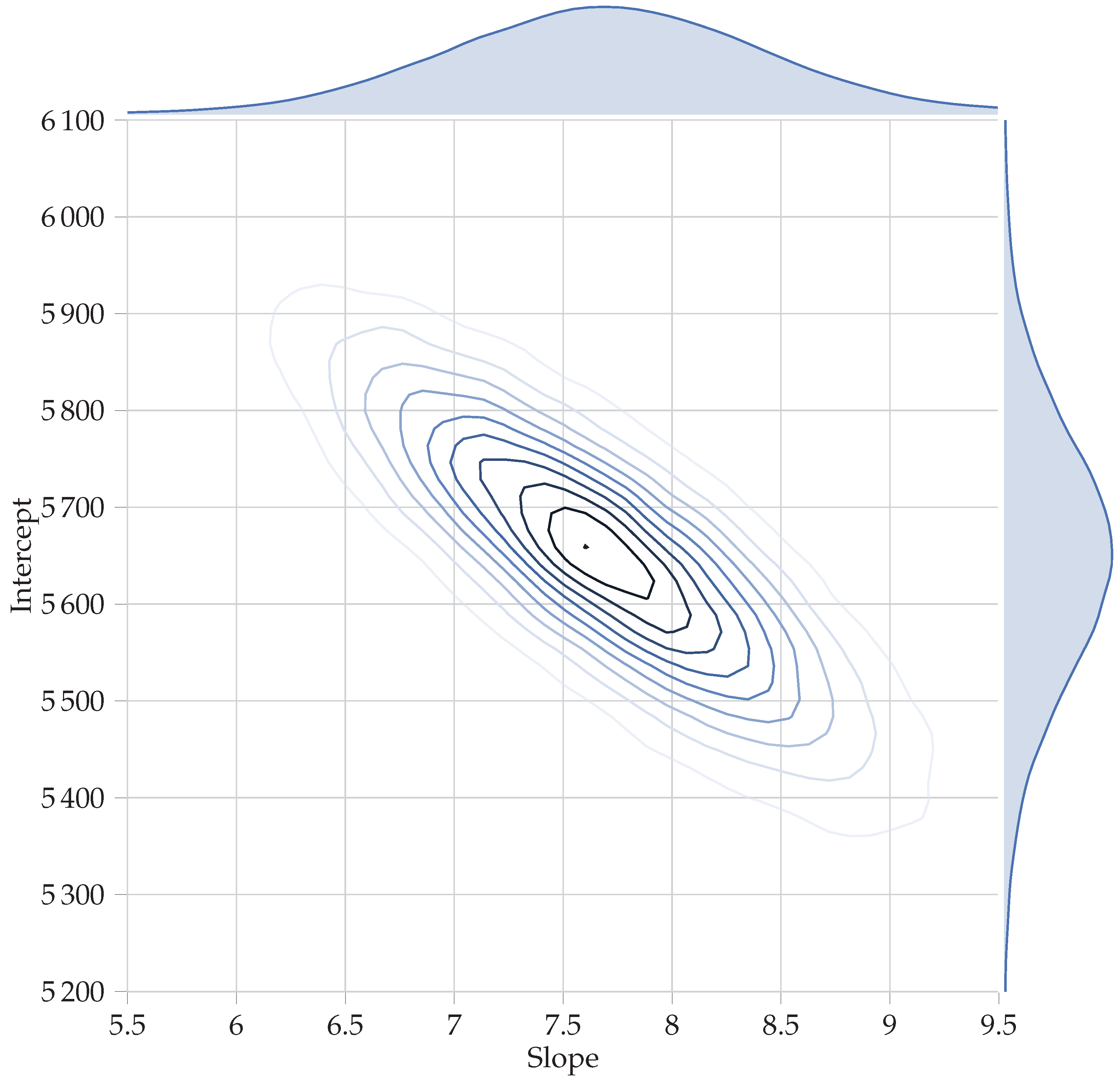
The MCMC results can be inspected in various ways. The posteriors on the parameters of interest are shown in
Figure 3. If a normal distribution is specified on the likelihood in Equation (
16) rather than the Student’s
t, the posterior means are identical to the linear regression point estimates—an expected result, since OLS regression is a special case of the more general Bayesian approach. Using a
t-distributed likelihood yields slightly different, but practically equivalent, results. The mean or mode of a given posterior is not of as much interest as the full distribution, since this full distribution will be used for any subsequent calculation. However, the mean of the posterior distribution(s) is given in
Table 3 for the curious reader.
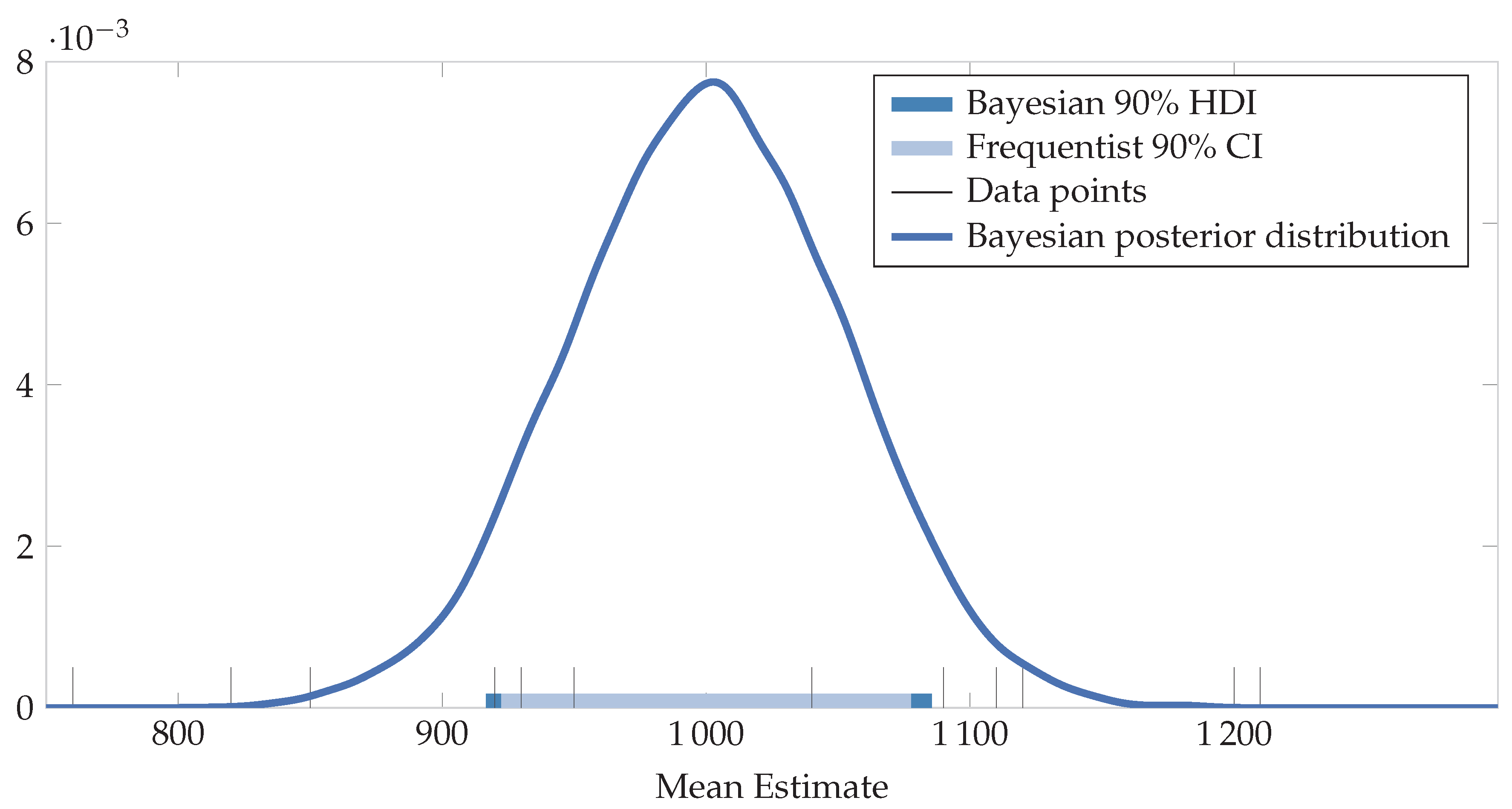
Two brief notes on Bayesian intervals are necessary. As discussed in
Section 1.1, the frequentist ‘confidence’ interval is a misnomer. To distinguish Bayesian from frequentist intervals, Bayesian intervals are often called ‘credible’ intervals, although they are much closer to what most people think of when referring to a frequentist confidence interval. The second note is that Bayesians often use HDIs, also known as highest posterior density intervals. These are related to the
area under the probability density curve, rather than points on the
x-axis. In frequentist statistics, we are used to equal-tailed confidence intervals since we compute them by taking the mean, and then adding or subtracting a fixed number—the standard error multiplied by the
t-value, for example. This works well for symmetrical distributions such as the Normal, as is assumed in many frequentist methods. However, real data distributions are often asymmetrical, and forcing an equal-tailed confidence interval onto an asymmetric distribution leads to including an unlikely range of values on the one side, while excluding more likely values on the other. An HDI solves this problem. It does not have equal tails but has equally-likely upper and lower bounds.
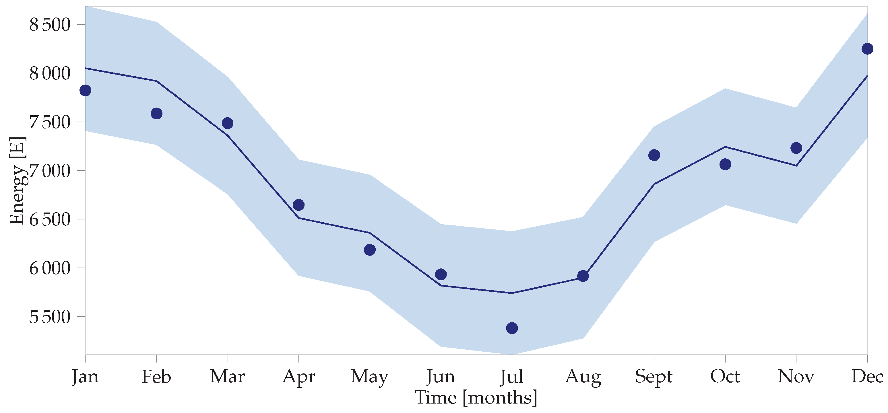
The posterior distributions shown in
Figure 3 are seldom of use in themselves and are more interesting when combined in a calculation to determine the uncertainties in the baseline as shown in
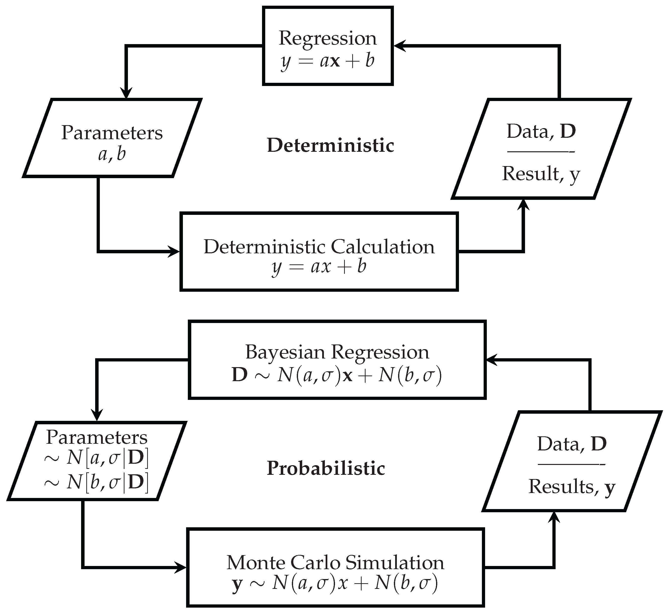
Figure 4, also known as the adjusted baseline. To do so, the posterior predictive distribution needs to be calculated using the
pm.sample_ppc() command, which resamples from the posterior distributions, much like the MC simulation forward-step of
Figure 1.
The Bayesian model can also be used to calculate the adjusted baseline, or what the post-implementation period energy use would have been, had no intervention been made. The difference between this value and the actual energy use during the reporting period is the energy saved. For the example under consideration, the IPMVP assumes that an average month in the post-implementation period: one with 162 CDDs. It also assumes that the actual reporting period energy use is 4300 kWh, measured with negligible metering error.
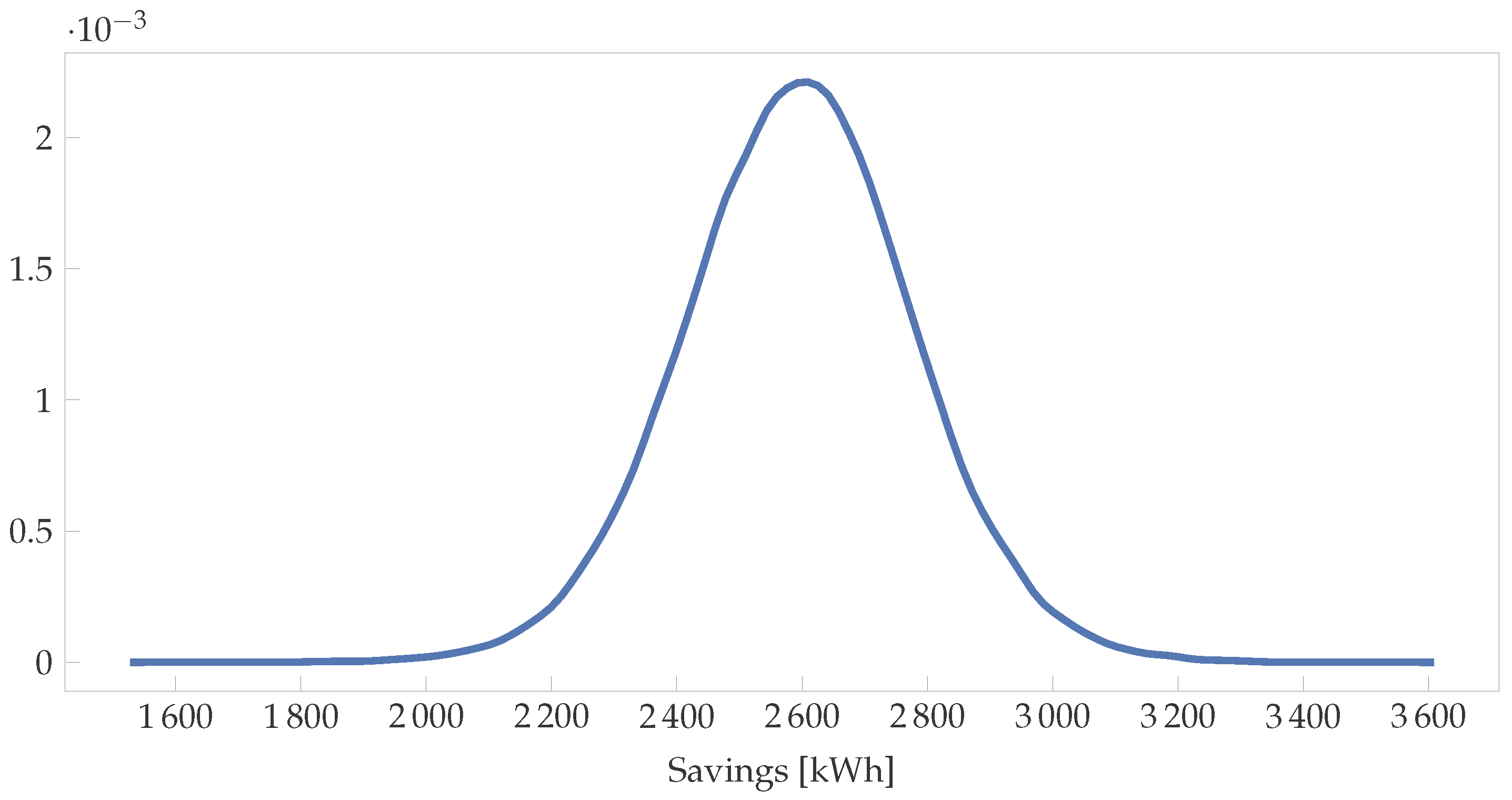
To calculate the savings distribution using the Bayesian method, one would do an MC simulation of:
where
and
are the distributions shown in
Figure 3. Note that they are correlated and so using the PPC method described above would be the correct approach. Running this simulation with 10,000 samples yields the distribution shown in
Figure 5. The 95% HDI is [2229, 2959], while the frequentist interval is [1810, 3430] for the same data—a much wider interval. Furthermore, the IPMVP then assumes averages and multiplies these figures to get annual savings and uncertainties. In the Bayesian paradigm, the HDIs can be different for every month (or time step) as shown in
Figure 4, yielding more accurate overall savings uncertainty values.
3.2.4. Robustness to Outliers
As alluded to above, using the Student’s
t-distribution rather than the normal distribution allows for Bayesian regression to be robust to outliers [
59]. The heavier tails more easily accommodate an outlying data point by automatically altering the degrees-of-freedom hyperparameter to adapt to the non-normally distributed data. Uncertainty in the estimates is increased, but this reflects the true state of knowledge about the system more realistically than alternative assumptions of light tails, and is therefore warranted. The robustness of such regression does not give the M&V practitioner carte blanche to ignore outliers. One should always seek to understand the reason for an outlier; if the operating conditions of the facility were significantly different, the analyst should consider neglecting (or ‘condoning’) the data point. However, it is not always possible to trace the reasons for all outliers, and inherently robust models are useful (Technical note: the treatment here is very basic, and for illustration. More advanced Bayesian approaches are also available. For example, if there are only a few outliers, a mixture model may be used [
60]. If there is a systematic problem such an unknown error variable, one can “marginalise” the offending variable out. The right-hand and top distributions of
Figure 3 are marginal distributions: e.g., the distribution on the slope, with the intercept marginalised out, and vice versa. For an M&V example of marginalisation where an unknown measurement error is marginalised out, see Carstens [
61] (Section 3.5.3). von der Linden et al. provides a thorough treatment of all the options for dealing with outliers [
3] (Ch. 22)).
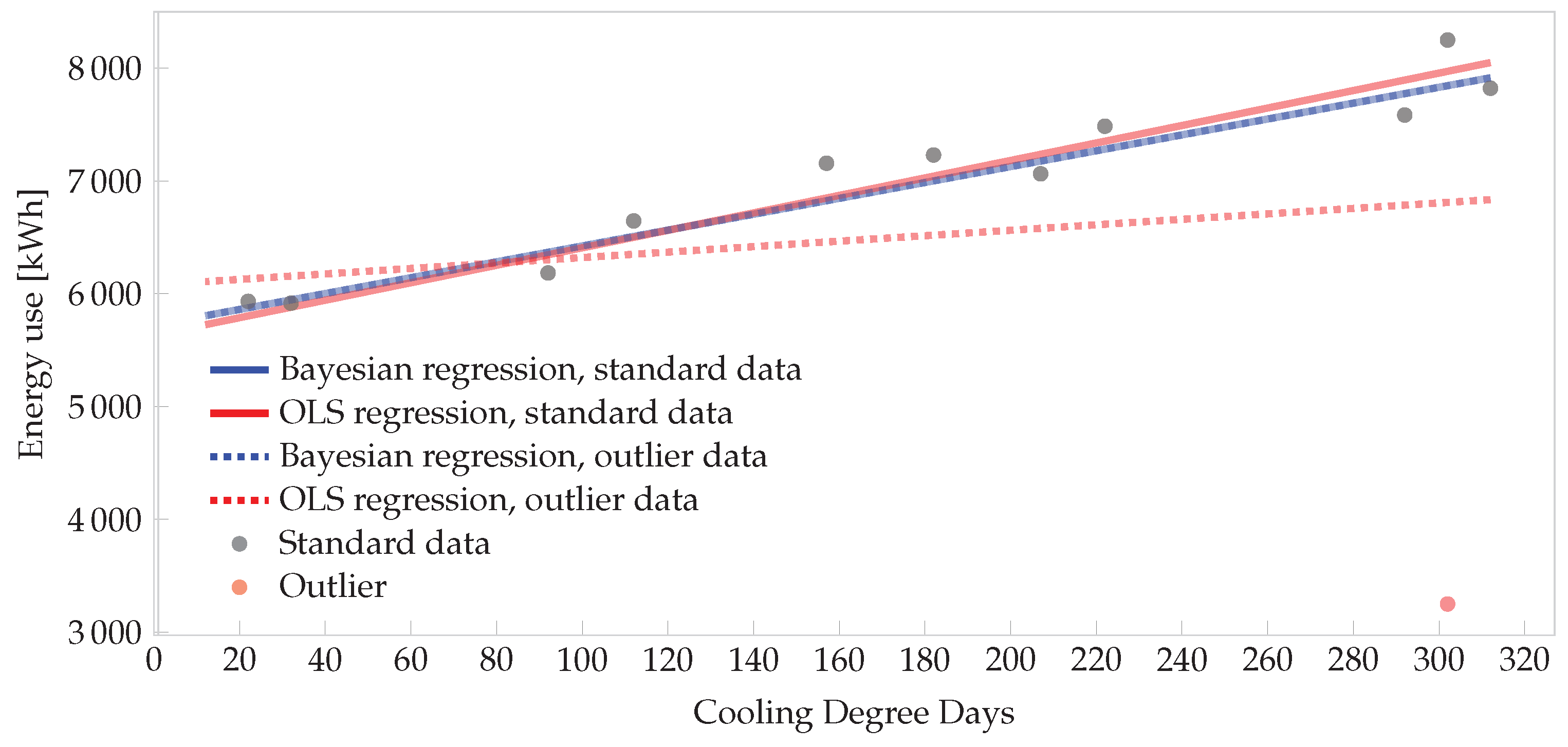
To demonstrate the robustness of such a Bayesian model, consider the regression case above. Suppose that for some reason the December cooling load was 3250 kWh and not 8250 kWh, indicated by the red point in the lower right-hand corner of
Figure 6. If OLS regression were used, and this point is not removed, it would skew the whole model. However, the
t-distributed likelihood in the Bayesian model is robust to the outlier. The effect is demonstrated in
Figure 6. Four lines are plotted: the solid lines are for the data set without the outlier. The dashed lines are for the data set with the outlier. In the Bayesian model, the two regression lines are almost identical and close to the OLS regression line for the standard set. However, the OLS regression on the outlier set is dramatically biased and would underestimate the energy use for hot months due to the outlier.


