3.1. Experimental Setup
Partial discharges are low-energy ionizations that occur inside the electrical insulation due to high electric field divergences within small volumes. The charge movement results in small current pulses with rise times as short as a few nanoseconds or even hundreds of picoseconds. The most common measuring techniques are designed to conduct these pulses through known paths where they can be acquired with high frequency current transformers or voltage dividers [
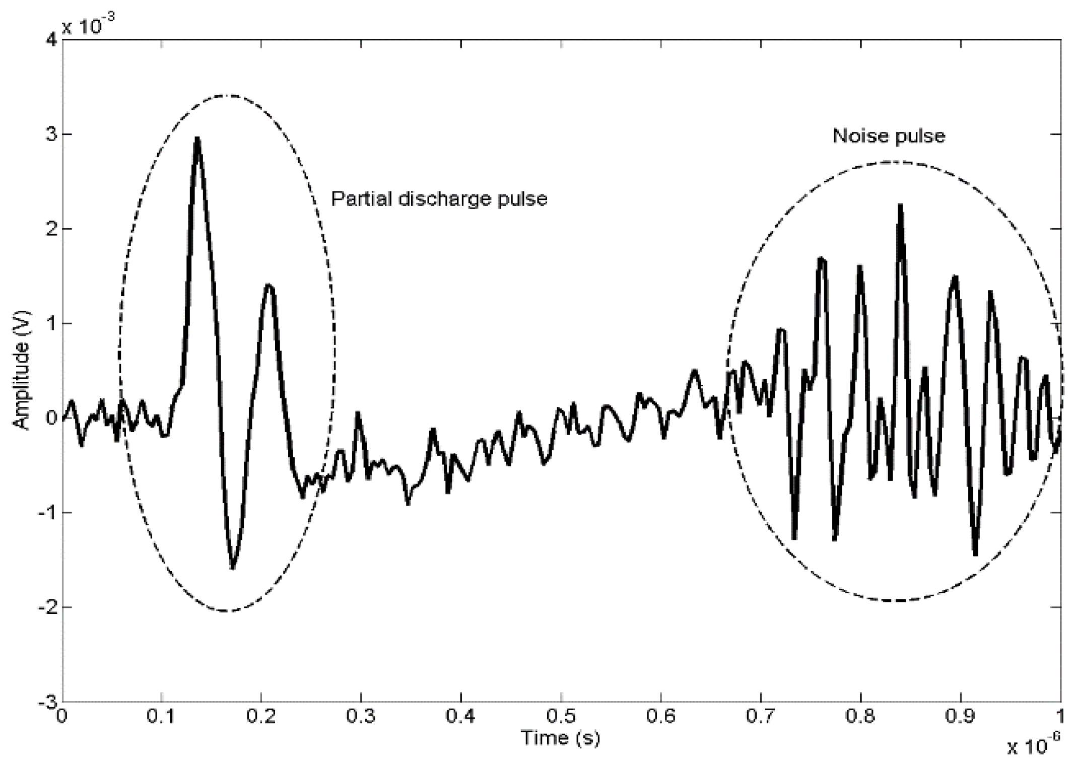
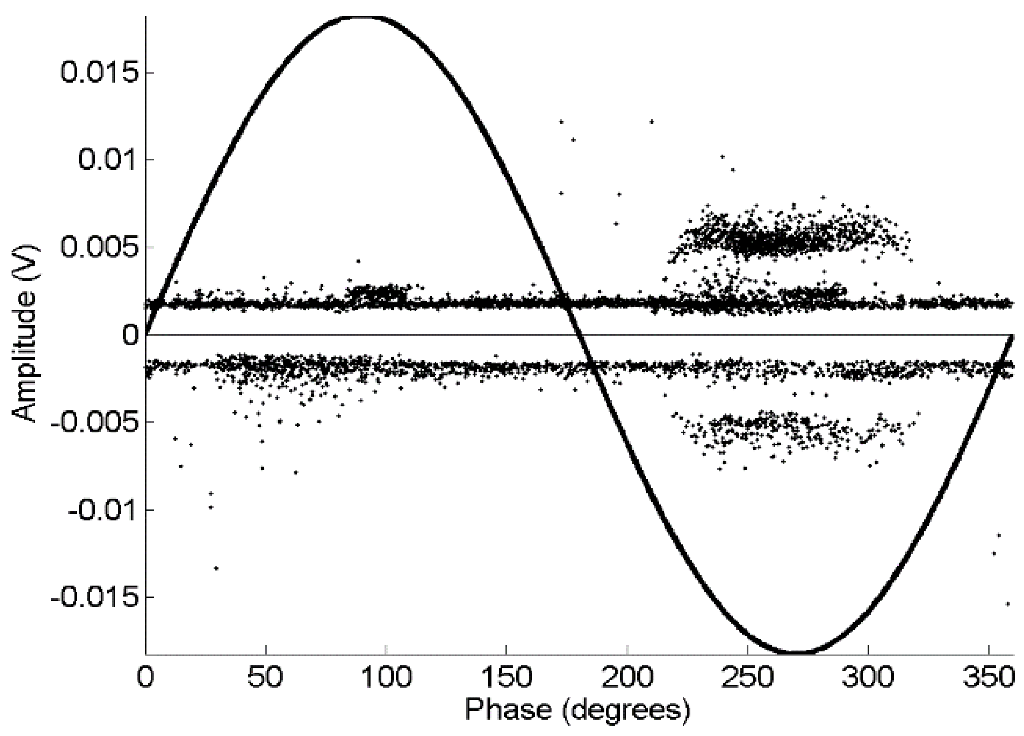
10]. The wires in the setup commonly filter higher frequencies limiting the band to some tens of megahertz resulting in signals such as that shown in
Figure 2. This figure shows a typical partial discharge pulse plus noise induced by the environment with similar energy as the PD.
Being partial discharges a stochastic process and the power spectral density strongly dependent on the layout of the measuring circuit [
8,
10,
27,
32], it is preferable and more realistic to create real events instead of using synthesized signals. Then, all data analyzed with the OCSVM, including partial discharges and noise have been collected experimentally with a detection circuit based on the standard IEC 60270 [
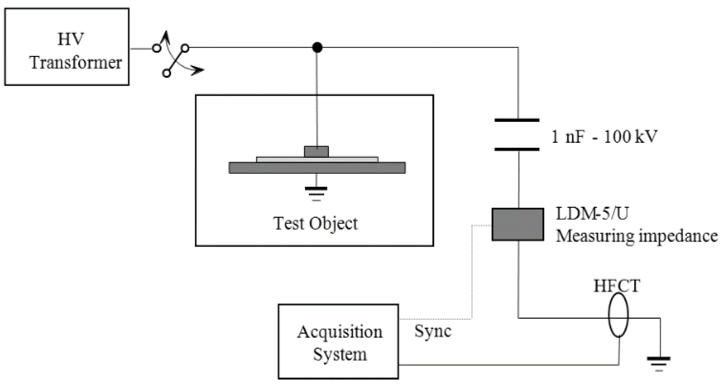
10]. This setup consists of a 750 VA transformer that applies high voltage to several test objects where partial discharges are created. A capacitive divider with a high-voltage capacitor connected in series with a measuring impedance provides a path for the high frequency currents generated by the PD pulses, see
Figure 3.
These transients are measured through a high frequency current transformer (HFCT) with a bandwidth up to 80 MHz. The measuring impedance gives synchronization to the grid frequency (50/60 Hz) so PD pulses can be plotted in conventional PRPD patterns. A NI-PXI-5124 digitizer (National Instrument, Madrid, Spain), with a sampling frequency of 200 MS/s, a resolution of 12-bit and a bandwidth of 150 MHz was programmed with Labview to automatize the acquisition of the pulses. The 50 Hz synchronizing voltage was connected to one of the channels and the other gets the waveforms of the high-frequency pulses. Every network cycle (20 ms), 4 × 10
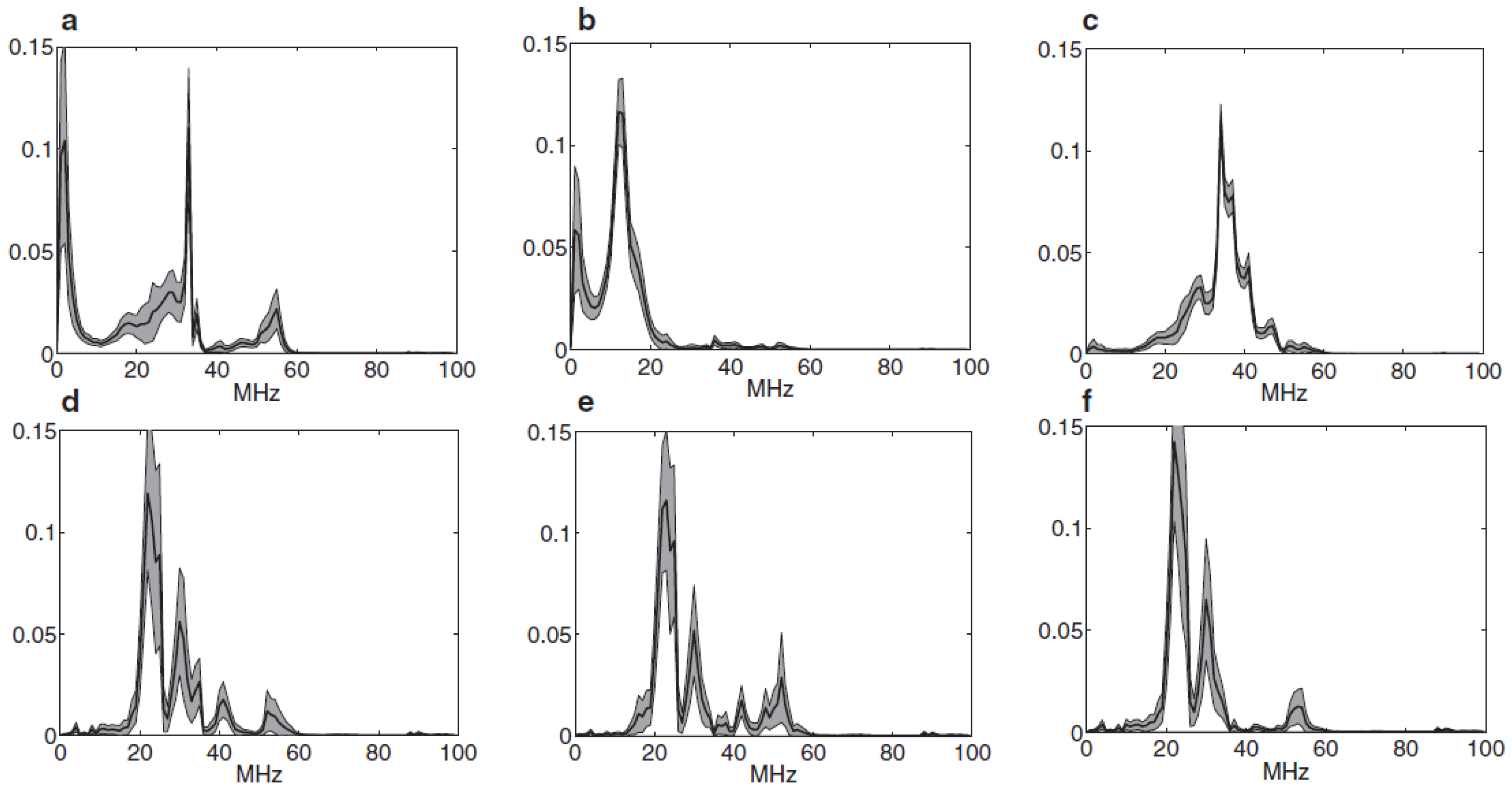
6 samples are acquired and split in time windows of 1 μs (sets of 200 samples) because it is not expected to have more than one PD pulse in this period. The maximum value of the signal and the time referred to the synchronizing signal are stored to plot the PRPD. Finally, the power spectral density of each signal is calculated and normalized to unit area before the analysis with the OCSVM (
Figure 4).
More details regarding the acquisition system can be found in [
11,
20,
33]. Five different test objects were used to generate the training and test sets for the OCSVM:
Point-plane experimental specimen: A 0.5 mm thick needle was placed above a metallic ground plane. The distance between the needle and the plane is set to 1 cm. In this test object, typical corona PD patterns are obtained once the ionization close to the needle tip is reached at 3 kV.
Insulating sheets immersed in mineral oil: This setup is designed to generate internal discharges and consists of three insulating sheets of NOMEX paper (polyimide 0.35 mm thick film). The central paper was pierced with a needle (1.05 mm in diameter) to create an air void inside this dielectric. The dielectric stack was inserted in a polyethylene envelope to create vacuum inside and the entire system was immersed in mineral oil to avoid surface discharges at low voltages [
11]. In this test object a stable internal discharges activity was found at 4.7 kV.
A joint test object: with the first two to create corona and internal discharges simultaneously at 4.7 kV. Notice, that placing two test objects in parallel gives a total capacitance which is the sum of the single capacitances; moreover, in this setup, three capacitive branches will be present for each high-frequency pulse, compared to the two of the previous experimental setups (measurement path and capacitance of the test object). All this makes the shape of the pulses different from the signals obtained with the test objects alone.
Contaminated ceramic bushing: A 15 kV ceramic bushing has been contaminated by spraying a solution of salt in water to create ionization paths along the surface. Clear surface partial discharges were detected above 14 kV.
A 12/20kV XLPE insulated power cable 12 m long: The cable was cut to have access to the main conductor and its insulation and shield was damaged to obtain a stable activity of partial discharges at its rated voltage.
The first four test objects are controlled insulation systems created specifically to obtain a certain type of PD and the corresponding background noise (or signals recorded in the default mode when the PD has not appeared yet). However, the fifth test object represents a faulted cable in which we expect to have partial discharges that will be classified accordingly to the results from the previous training sets.
Three measurement sets were done for every test object. One set at low applied voltages and low trigger levels to record noise only. Another set, increasing the voltage to a value above the partial discharge inception voltage, where PD activity was found to be stable; the trigger is set high so the data only contains partial discharges. Finally, another set at high-voltage and low trigger as in the first set to have PD and background noise simultaneously (an example of their PRPD is presented in
Figure 5, where it is shown the difficulty of making diagnosis from this classical representation).
After all the process there are three files: the first contains background noise pulses only, the second, partial discharges only, and the third, PD blended with noise 4). The first two are used to train the classifiers and the last one is used to test the separation capability of the system. The experimental setup is carefully maintained invariant so its equivalent capacitance does not change during all the process and all signals are acquired in the same conditions so we can do a reliable parametrization.
Table 1 summarizes the sizes of the datasets recorded from these experiments.
As explained before, plotting the pulses in a PRPD graph helps to know by simple visual inspection if the decisions made by the OCSVM are correct.
With respect to the training of the OCSVMs, we have followed a very standard approach. The OCSVMs are endowed with the KL-based kernel of
Section 2.2, whose width parameter
is selected in a logarithmic scale between 0.5 and 50. The regularization parameter
is also selected in a logarithmic scale between 0.005 and 0.2 (anyway we checked that the optimum never occurred in the extremes of the ranges). The tuning of these two parameters is carried out by tenfold cross validation in a grid search. The bias term of each OCSVM,
, was fixed so that all the samples of the target class in the training set scored a positive number.
3.2. Results
The first set of results illustrates how in fact noise models can be shared across different PD scenarios.
Table 2 displays the efficiency when detecting default mode when the OCSVM is trained using background noise signals (without PD) recorded in a particular experiment of PD (each row corresponds to a training set scenario) and tested using default mode signals recorded in a different PD experiment (diagonal terms are trivial since the training and testing sets are indeed the same set).
Nine out of the twelve non-diagonal accuracies in
Table 2 are above 90%, one is above 86% and only the cases involving test background noise signals of the experiment with simultaneous PD present really poor detection rates.
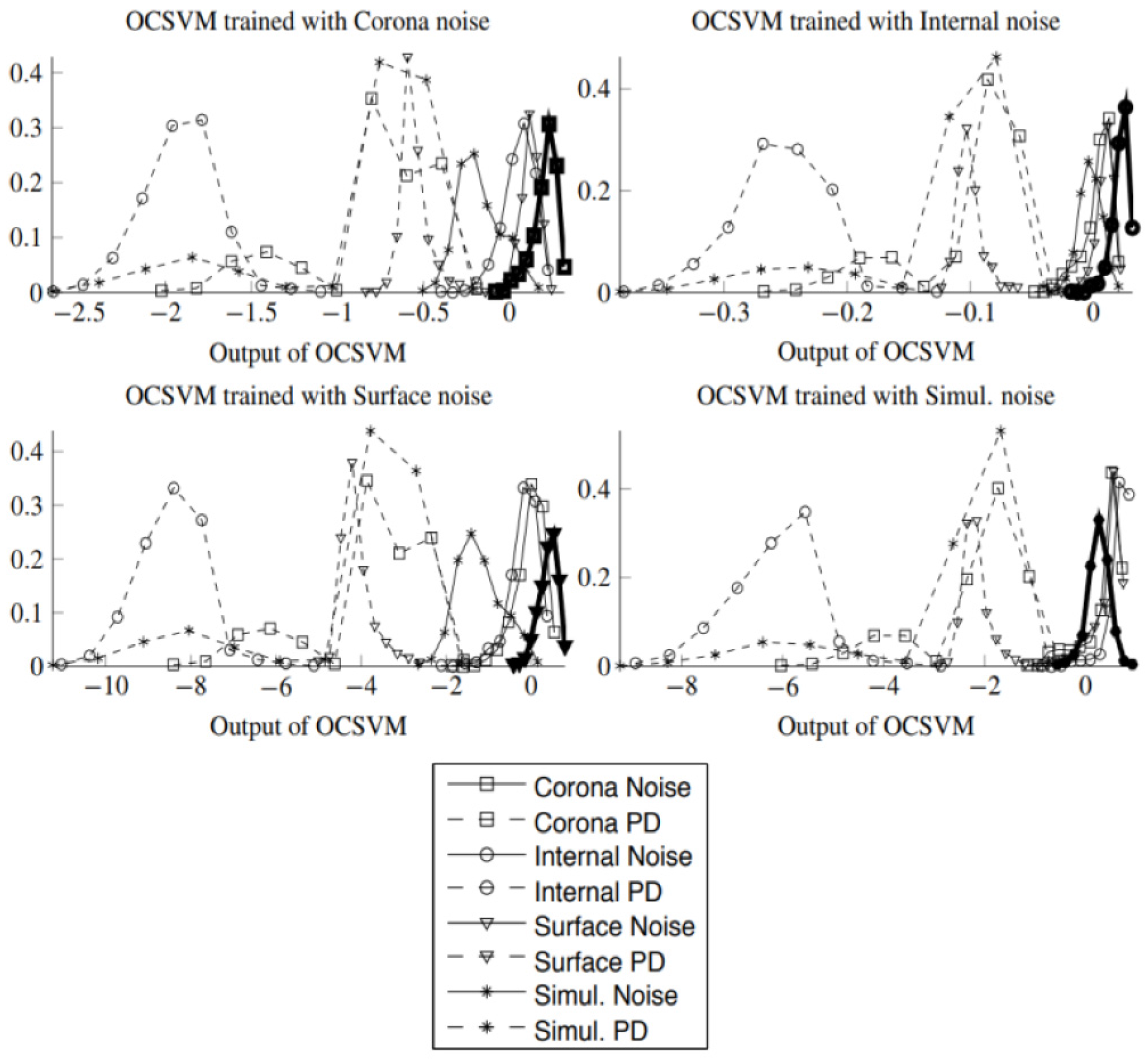
Figure 6 shows the normalized histograms (the normalized histogram is an approximation to the probability density of the output of the OCSVM. The range of values of the output of the OCSVM is divided into equally sized bins and the histogram value in each bin is the count of the number of test samples for which the output of the OCVSM falls in that bin. The values of the bins are then divided by the number of test samples so that they add up to one and thus this normalized histogram can be used as proxy for the probability density) of the scores of the OCSVM trained with the different background noise records and tested using files coming from different experiments that contained either pure background noise (solid lines) or pulses of a single type of PD (dashed lines). The OCSVM outputs for background noise appear highly overlapped independently of the particular noise used to train the model and the outputs for PD pulses appear well separated from the outputs corresponding to noise. In two cases (using the training data from corona and surface setups) the background noise from simultaneous PD (Simul.Noise in the plots) appears slightly shifted towards the negative part of the histogram, although clearly separated from the PD pulses. Notice that being noise, the plots should have entirely been in the positive range of the histogram. Nevertheless, these lines are clearly separated from the dashed plots corresponding to PD which supports the suitability of the OCSVM as core algorithm for a detector that is capable of being adapted to another PD scenario.
In order to justify the election of the default mode model for domain adaptation we have repeated the modeling in
Table 2, but now using only PD pulses without noise to train the OCSVM. The aim in this new set of results is to say if a certain pulse is a PD or not.
Table 3 presents these results. The structure of
Table 3 is very close to an identity matrix (excepting the tests results for corona and internal PD when training is made with the simultaneous source), pointing out the fact that each type of PD is consequence of a different physical process and therefore the shape of the PD pulses is different for each experiment, which significantly reduces the usability of a one class modeling when the target class is a particular type of PD source. A good illustration of this fact is the results of internal and corona when the OCSVM is trained with the Simul. training set: the OCSVM treats both types of PD as members of a same class. These results from
Table 3 are in agreement with previous works [
11], where it is proven that, for the same experimental setup, each PD source has a characteristic frequency response;
Figure 4 shows this situation too.
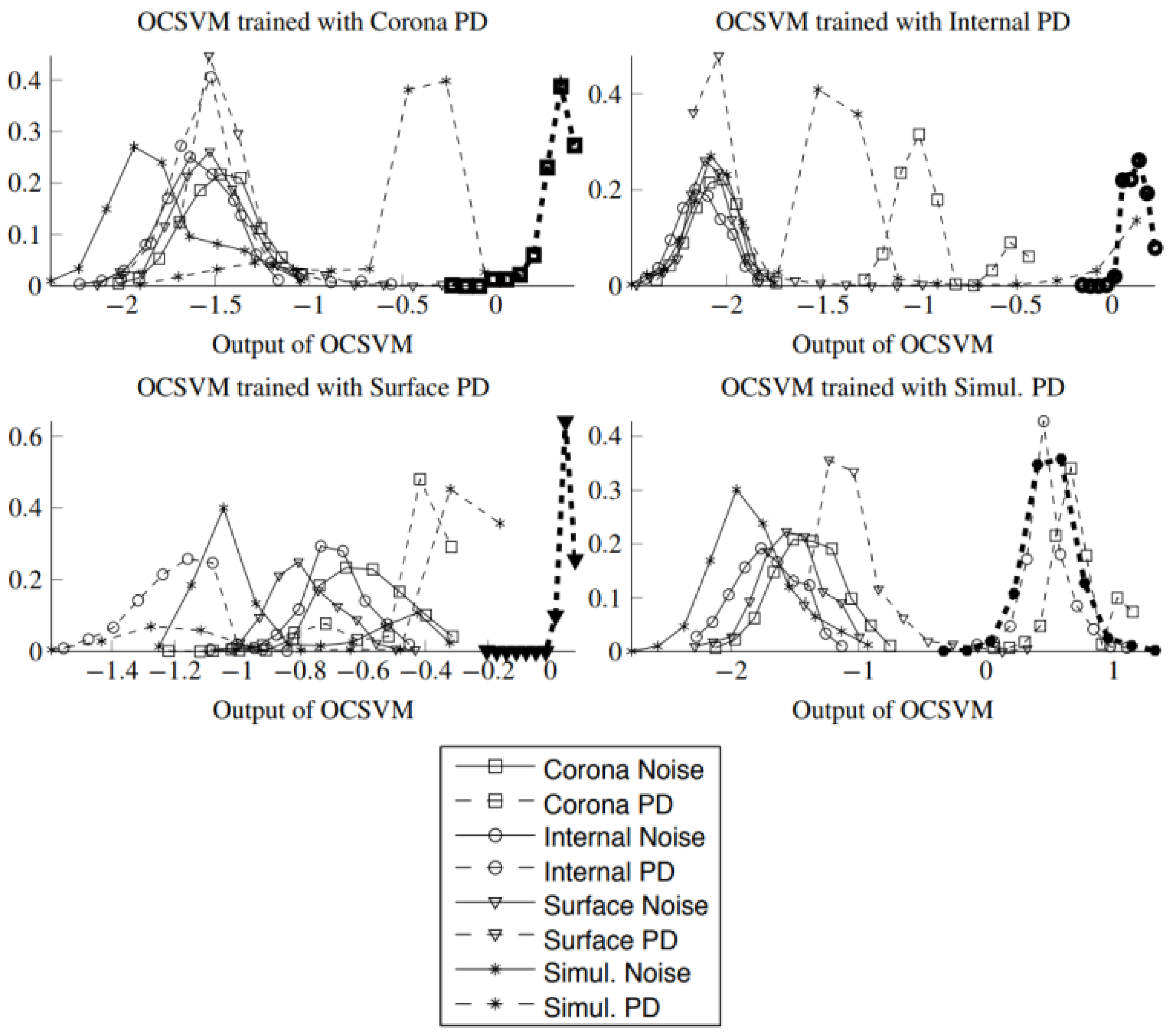
Figure 7 displays the histograms of the OCSVM trained with the different types of PD. In a few of these cases, the histograms of the outputs corresponding to PD test pulses (dashed lines) show that the
f(
x) score could potentially be used to discriminate PD, but in general the OCSVM based on learning the distributions of PD pulses are more difficult to adapt to other scenario than the models based on learning the background noise distribution. Moreover, the noise histograms (solid lines) appear again highly overlapped in the four cases, illustrating the fact that the noise is more homogeneous across experiments and that a model trained with default mode pulses from a given scenario could be easily adapted and achieve a good performance in a different scenario.
The next set of results, displayed in
Table 4, illustrate the detection capabilities of the OCSVM trained with a single type of background noise and tested with a set that includes both PD and noise pulses recorded simultaneously in different PD generation scenarios. The label assigned by the OCSVM to each pulse is compared with the label that would assign a binary Support Vector Machine (SVM) trained with a set of pure PD and pure background noise pulses recorded in the same scenario as the test set. The SVMs are endowed with the same kernel as the OCSVM. According to our past experience [
20] this binary classifier is able to almost perfectly discriminate between PD and noise, so its label assignments can be perfectly considered as ground truth.
Figure 8 shows the identification of pulses made with binary support vector machines.
Table 4 displays indeed two sets of results. For each training set, we have used two strategies to fix
in Equation (1):
Without domain adaptation (top row for each training set, labeled no d.a.): The value of is determined after the optimization of (2) subject to (3) and (4). This way all the noise samples in the training set produce a positive value in the output of OCSVM.
With domain adaptation (bottom row for each training set, labeled d.a.): The value of obtained from the optimization of (2) subject to (3) and (4) is refined using a second training set composed of noise pulses recorded from the same scenario in which the testing set was recorded. The value of is modified so that all the instances in this second training set produce a positive output in the OCSVM.
The domain adaptation is the simplest re-calibration that one could introduce in a realistic scenario in which the initial training set is not rich enough to represent the target class. The OCSVM score relies on the kernel functions centered on the support vectors and on the bias term . This re-calibration involves the use a second training set of background noise pulses to fine tune the value of . Notice that, like the initial set, this training set is not labelled at all, one just need to ensure that it was recorded under PD-free conditions, and this requirement is easy to fulfill in an industrial application. This way, the learning still falls into the one class paradigm as the recalibration does not demand a labelled data set.
Table 4 shows that the OCSVM with the first strategy makes good predictions in almost all the experimental setups, excepting some cases with simultaneous discharges (the same with lower identification capabilities shown in
Table 2), while the strategy with domain adaptation achieves a very good classification in all scenarios.
The final set of results involves the analysis of signals recorded in a very different experiment, closer to a real-world scenario. This is the case of a portion of an XLPE cable connected to high-voltage and inducing a source of PD by deteriorating the insulation in one site. The equivalent capacitance of this setup is remarkably higher than those of the other test objects because the length is 12 m so high-frequencies of the PD pulses are strongly attenuated.
Table 5 shows the agreement between the labels assigned by the OCSVM models learned in the previous experiments (using the noise signals termed as Corona, Internal, Surface and Simultaneous) and the labels assigned by an OCSVM trained using background noise pulses recorded at the cable experiment. As before, the top row in
Table 5 displays results without domain adaptation (the value of
is fixed using the same noise that was used to train the OCSVM), whilst the bottom row displays results with domain adaptation. This domain adaptation consists in using the same model but refining
for each OCSVM with the set of noise pulses recorded in the cable experiment.
The results in
Table 5 show again that the domain adaptation involving the tuning of
works really well independently of the default mode signals used to construct the OCSVM model. In this particular case, as the change in equivalent capacitance of the test object has been more pronounced than in the other cases, the tuning of the parameter
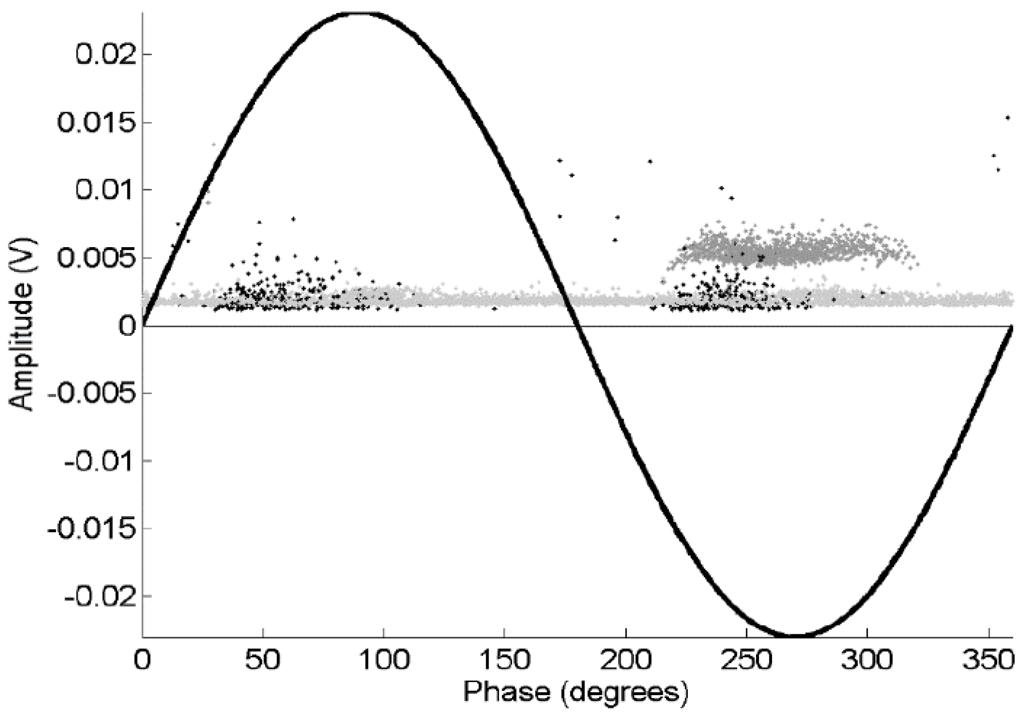
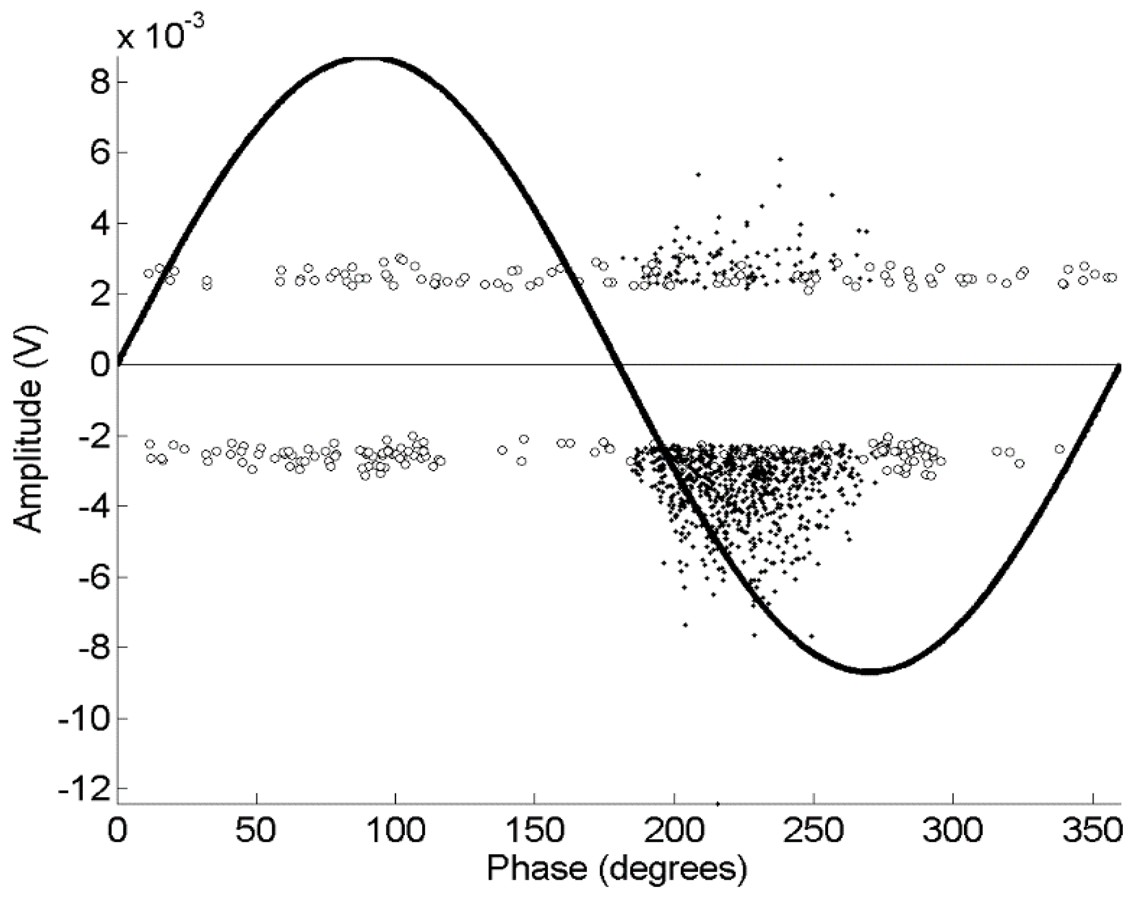
is more convenient than in the previous experiments to obtain a convenient identification. Moreover, the PRPD in
Figure 9 shows that the events classified as noise (with circles) do not have correlation with the phase of the 50 Hz sinusoid whereas black points, that are not-noise pulses, have a clear correlation appearing only on the negative semi-cycle, which means that they are PD. This means that the discrimination has been done correctly. It is interesting to note that some PD (not-noise) pulses have magnitudes similar to noise pulses, which means that this technique can be quite useful to detect PD signals in testing setups with low signal to noise ratio. This is very important, since these low-magnitude PDs (events whose probability of occurrence is higher than high magnitude PDs) could have been discarded if the trigger level had been raised to reject noise, leading to possible mistakes in the assessment of the status of the power cable.
Finally, it is worth discussing the capabilities of the OCSVM to deliver data models that are not difficult to interpret by human operators. The lack of interpretability is one of the main handicaps that face the introduction of machine learning techniques in industrial applications. In the problem under study, the OCSVM models are a linear combination of kernel functions centered on some of the training instances (the SVs). It turns out that the obtained models are very sparse in terms of the number of training examples that end up taking part in the OCSVM.
Table 6 displays the size of the models in terms of data examples. In most of the cases the size of the detector is quite small. Therefore, the analysis of the classification of a test signal
xt in terms of the linear combination in
f (
xt) would first bring out which SVs are more similar to
xt under the metric defined by the kernel. Then the human operator could approximate the outcome of the OCSVM as a combination of the expected output for each of these more similar SVs. Moreover, since the kernel captures similarities in the shapes of the PSDs, those frequency bands in which the shapes of the test signal and of the SVs PSDs are closer would become the key to the interpretation of the classifications.

 ,
, 


