3.1. Model Development
The model developed for the system analysis is based on an existing system model by Schimpe et al. [
7]. The model is developed for holistic energy efficiency evaluations of container-size to utility-scale battery storage systems. Separate component models are implemented and coupled to an overall system model.
The existing model is adapted to the specific system structure and parameters for all components of the specific system are implemented.
Table 1 shows the grouped components of the system, their respective component model type as well as the main parameters used for the model parameterization.
The battery-pack, part of the TU, is modeled based on a single-cell model. The cell is simulated through an equivalent circuit model featuring an open circuit voltage
as well as a resistance
, which accounts for the overvoltages within the cell. The resistance parameters are derived from pulse parameterization for both directions of current
, charge (positive) and discharge (negative). The battery packs are water-cooled and stored at approximately 20 °C ambient temperature, and operate at a low average load as will be discussed in
Section 3.2. The cell temperatures are thus expected to not increase in temperature strongly. As thermal parameters of the cell and pack are not available, the cell parameters, open circuit voltage and resistance values, are taken and implemented at a temperature of 25 °C versus the State of Charge
SOC. Mismatching losses in the series-connection and increases in battery cell resistances due to cell degradation are not implemented, as no information is available, but in general, are both expected to increase losses.
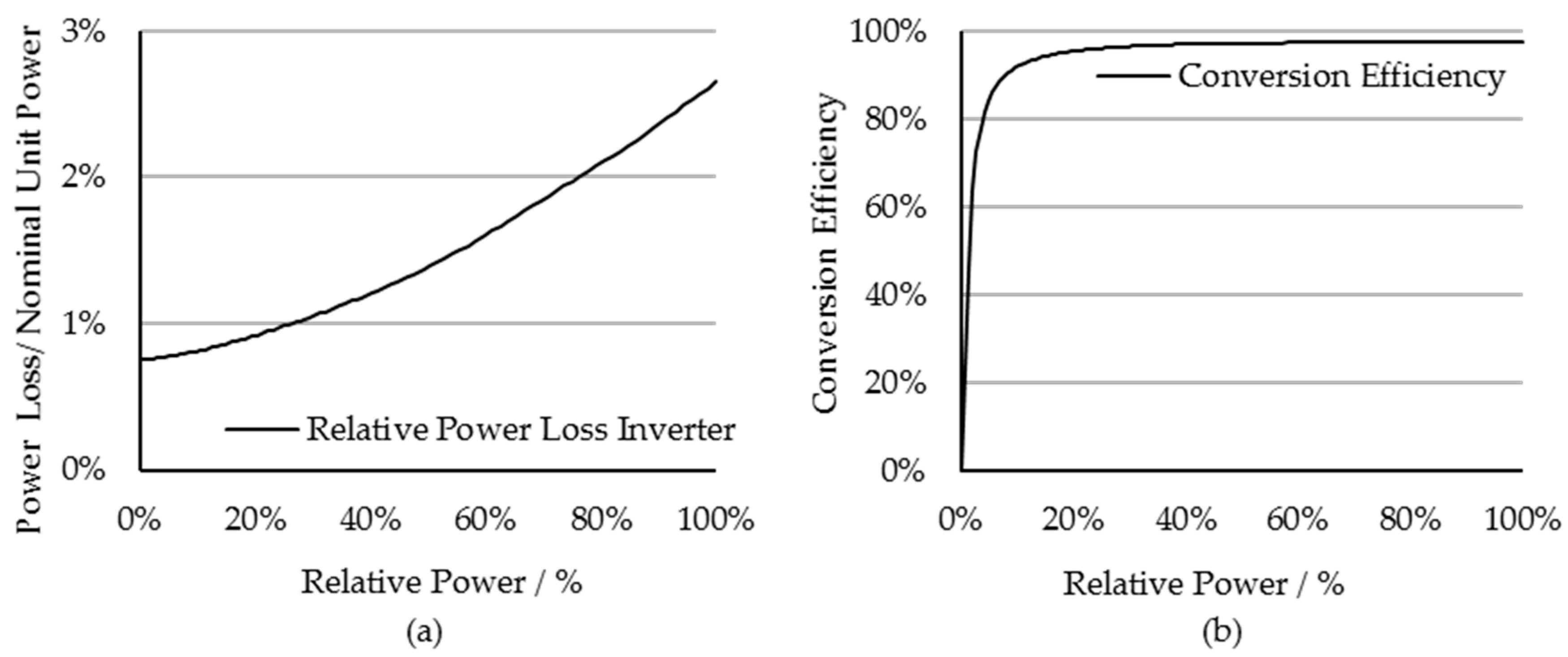
The second component model of the TU, the PE model, is implemented through look-up data of the power losses as function of the power, . The data, which is provided for each PE type by the PE manufacturer, is implemented with separate data for both power flow directions, charge, as well as discharge. Power factor is set to 1 for both system operation providing PCR as well as in the measurements of the power loss curves.
The transformer connecting the overall system to the grid is modeled based on measured data for the power loss at both no-load and full-load, which is provided by the transformer manufacturer. The transformer losses are then calculated with a square-power function for the load-dependent losses, which feature Ohmic loss behavior, as function of the secondary-side power .
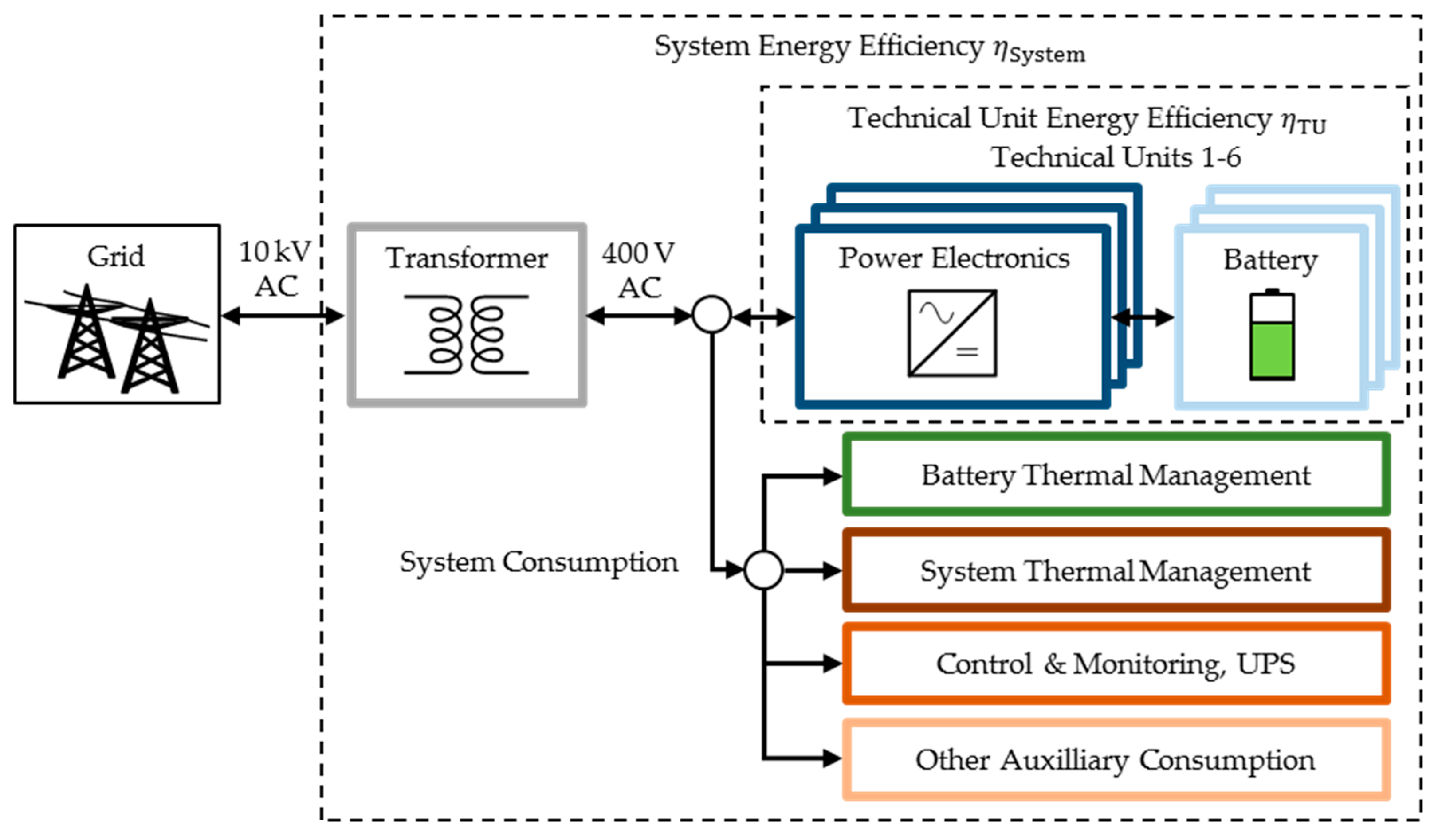
The auxiliary components are not modeled but implemented through measured data for their power consumption. Four groups are defined: (I) Battery Thermal Management System (B-TMS); (II) System Thermal Management System (S-TMS); (III) Control and Monitoring components that include the Uninterruptible Power Supply (C&M); and (IV) the remaining consumption for various components. Detailed measurements of the remaining various components are not available; however, a large share of consumption is assumed to be attributed to ambient air filter components. For each auxiliary component group, the measured power consumption is implemented as function of time .
The power control of the system is implemented as the load profile for each TU, based on the measured data over time, . The SOC measured in each TU (average SOC for a TU with two power strings), , is set as initial value for the simulation after every 24 h to remove SOC drift between the model and the system due to small deviations for the battery current, which add up over long simulation durations. The changes in SOC through the reset are included in the loss calculation.
3.2. Simulation Results
Before analyzing the energy losses of the complete system, the TU model is validated against measured data. The measured efficiency values here and in the following include the differences of stored energy through the changed battery SOC between the beginning and the end of the considered period.
Table 2 shows the charged/discharged energy of the TU, and the simulated/measured round-trip energy efficiency and their deviation for the month of March 2017.
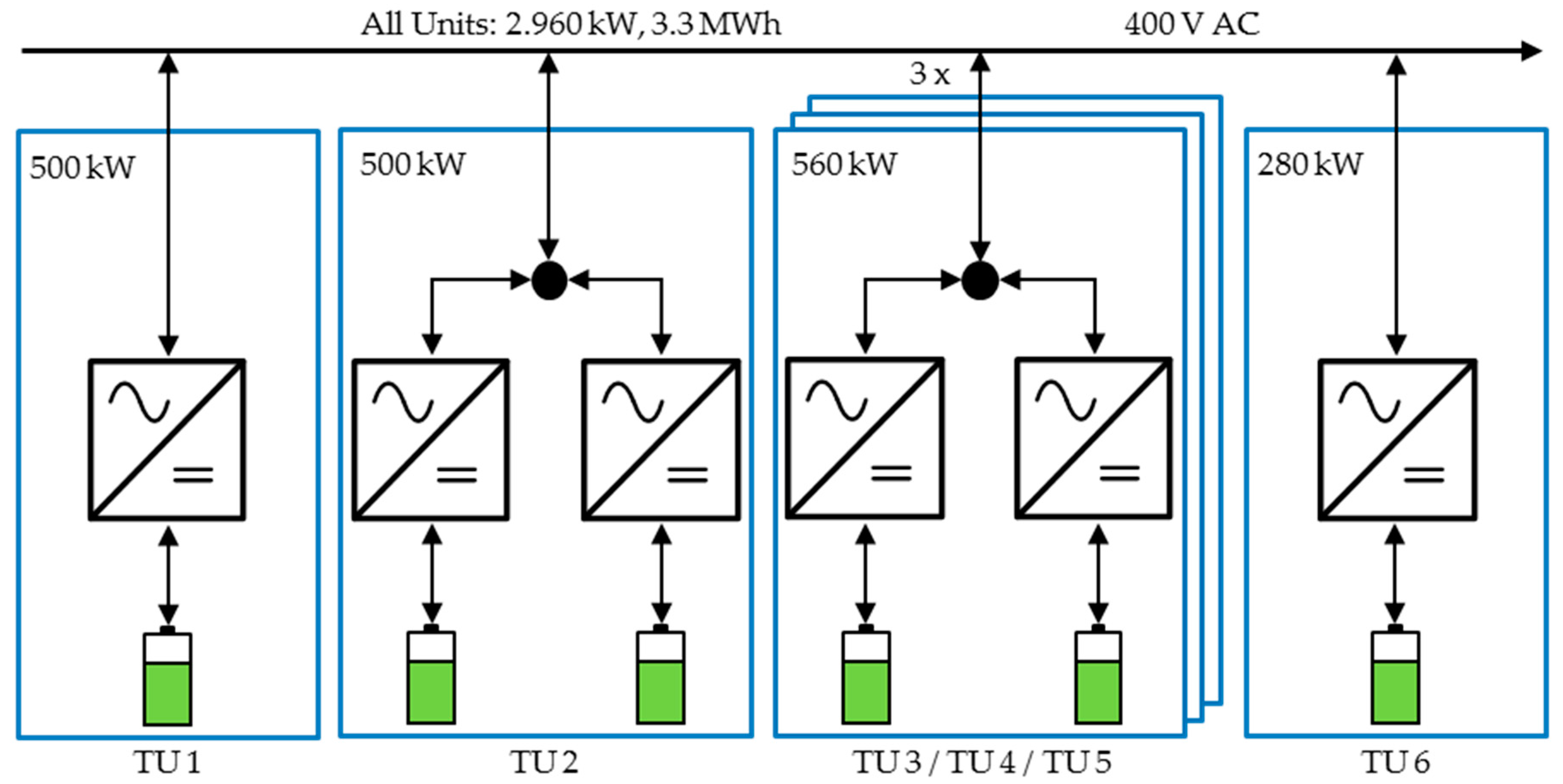
Energy throughput for TU 2–6 varies with the respective unit power. TU 1, the backup unit, is rarely active for inter-system balancing operation. TU 2–6 providing PCR show similarly measured efficiencies between 72.88% and 76.65%. The different efficiencies are caused by technical setup variations, such as varying battery types, which are each implemented with specific parameters, and different inverter sizes (see
Figure 3). TU 1, the backup unit, is active at only low relative power and thus has a relatively low efficiency.
The simulation results for the energy efficiency of the various TU are between 0.16% and 2.37% higher than the measured values. This trend in the deviation results possibly from the battery model. In the implemented type of equivalent circuit model, all battery overvoltages under load are calculated based on the single resistor in the model. Battery overvoltages are, however, dynamic, increasing with longer durations of load [
27]. A battery operating under fluctuating load thus operates with decreased overvoltages compared to a battery model using a non-dynamic resistor only. Finally, the accuracy of the power electronics parameters for the power loss curve can significantly influence the model result.
All units in total have a measured efficiency of 73.25% for which the simulation predicts an efficiency of 71.77%, equating to a deviation of −1.48%. Summarized, the model is in good agreement with the measured data for the system.
When considering the complete system, the round-trip energy efficiency is found significantly lower at 56.06%, again for March 2017. The reduction is due to the additional energy losses in the transformer (1.79 MWh) as well as due to the auxiliary energy consumption (B-TMS 1.47 MWh, S-TMS 2.57 MWh, C&M 7.88 MWh, Other 1.18 MWh).
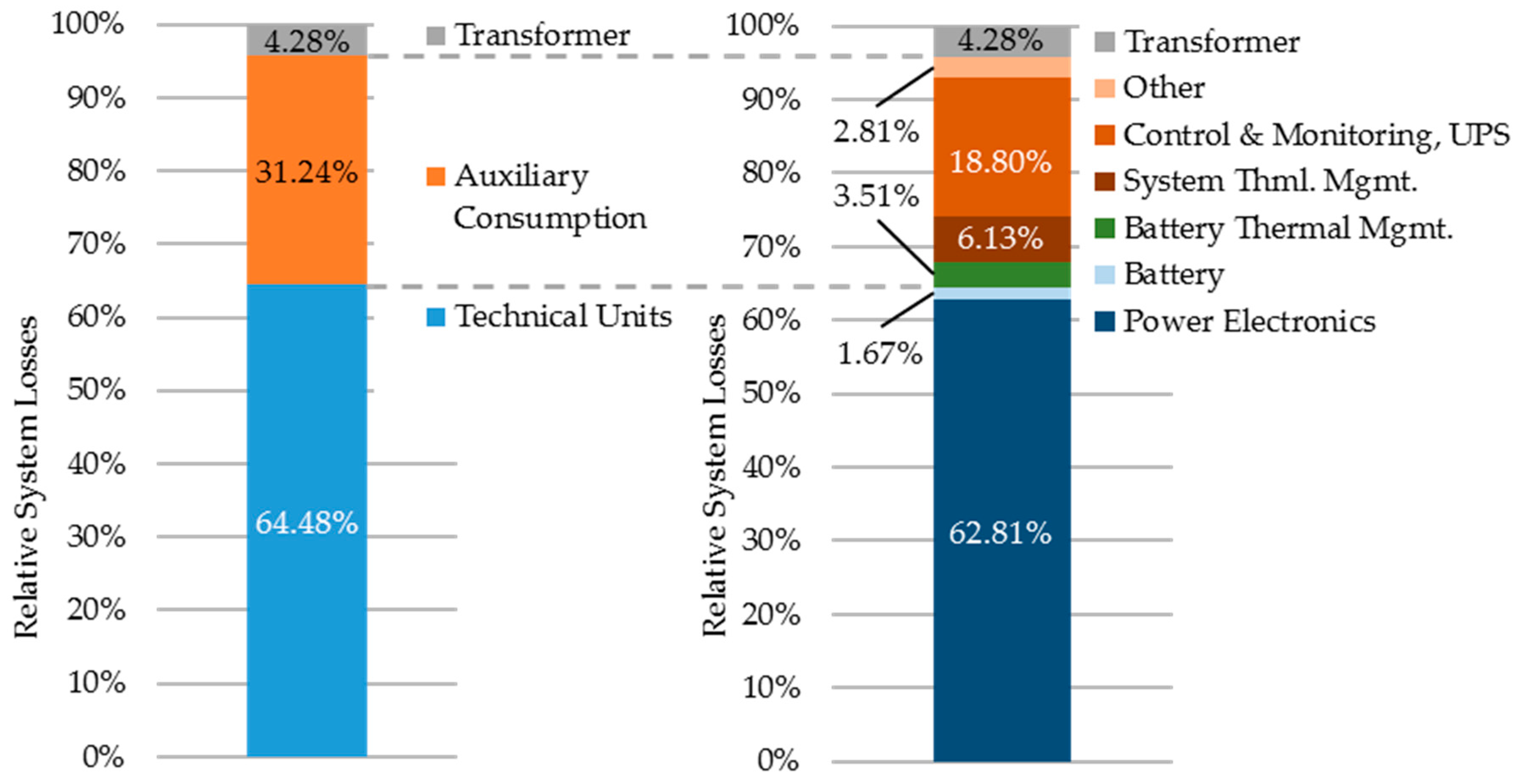
To identify the exact mechanism, the loss distribution analysis for the complete system is conducted and shown in
Figure 4 for the operation presented in
Table 2. The left side shows the distribution grouped by transformer losses, auxiliary consumption and the losses occurring in the TU.
With 64.48% of the overall losses, the TU are responsible for most losses. Second is the auxiliary consumption, which leads to 31.24% of all losses. The transformer’s share of losses at 4.28% is here the smallest contributor.
The right side shows the analysis with a more detailed breakdown. Within the TU, the PE is identified as the largest contributor, whereas the batteries are the smallest contributor of all loss mechanisms. The breakdown of the auxiliary consumption shows that all components are relevant contributors. The Control and Monitoring of the overall system, which also includes the power consumption of the uninterruptible power supply, is the biggest contributor to the auxiliary consumption and the second-largest in overall. It is noted that the energy consumption of the thermal management is subject to changes with varying outdoor temperatures and that this analysis specifically covers March 2017 only.
As the model represents the auxiliary consumption only as measured data, no improvement strategies for the auxiliary consumption of the given system through improved operation can be evaluated. The transformer is a passive component and thus also offers no improvement potential through operational strategies. Consequently, an improved operational strategy derived from the analysis in this work will focus on the TU operation, which is the largest contributor to the system losses as the previous analysis has shown.
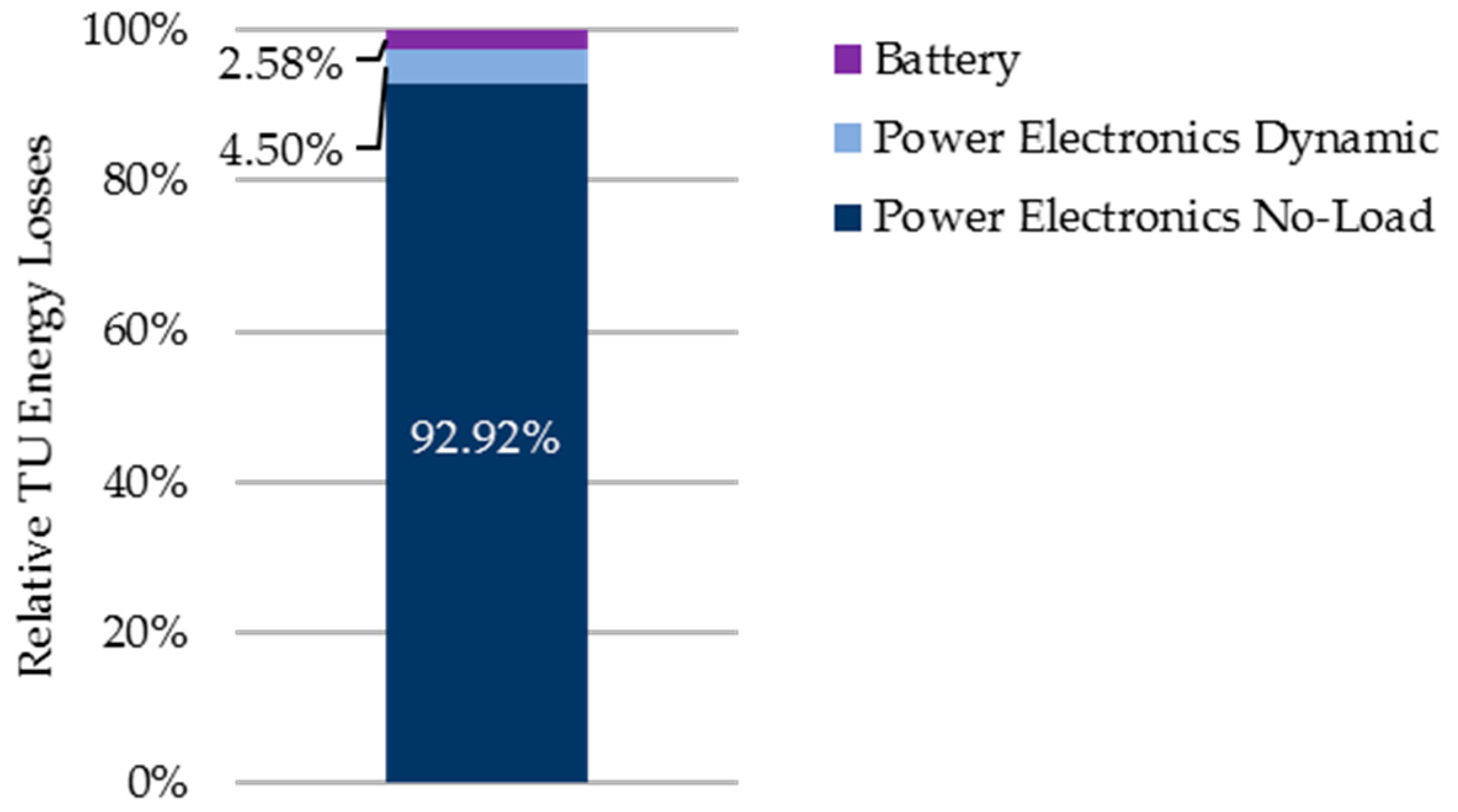
Figure 5 shows the loss distribution for all TU. Here the differentiation between
no-load losses and
dynamic losses for the PE is made. Losses within the PE are the sum of switching and conduction losses within the semiconductors, magnetic losses in filter components, and Ohmic losses in general. As no detailed PE model is available, the losses are grouped into no-load losses and dynamic losses. No-load losses are defined as the power losses occurring at no output power, but with the PE unit in operation, fully connected to its AC and DC sources, and with the switching control active. Dynamic losses are defined as the losses that occur additionally to the no-load loss value when the unit increases its output power.
The analysis shows that in total the no-load losses lead to 92.92% of the overall losses of the TU. The battery losses and the dynamic PE losses are in comparison much smaller.
For further evaluation of the origin of losses in the TU, the profile of the application is analyzed.
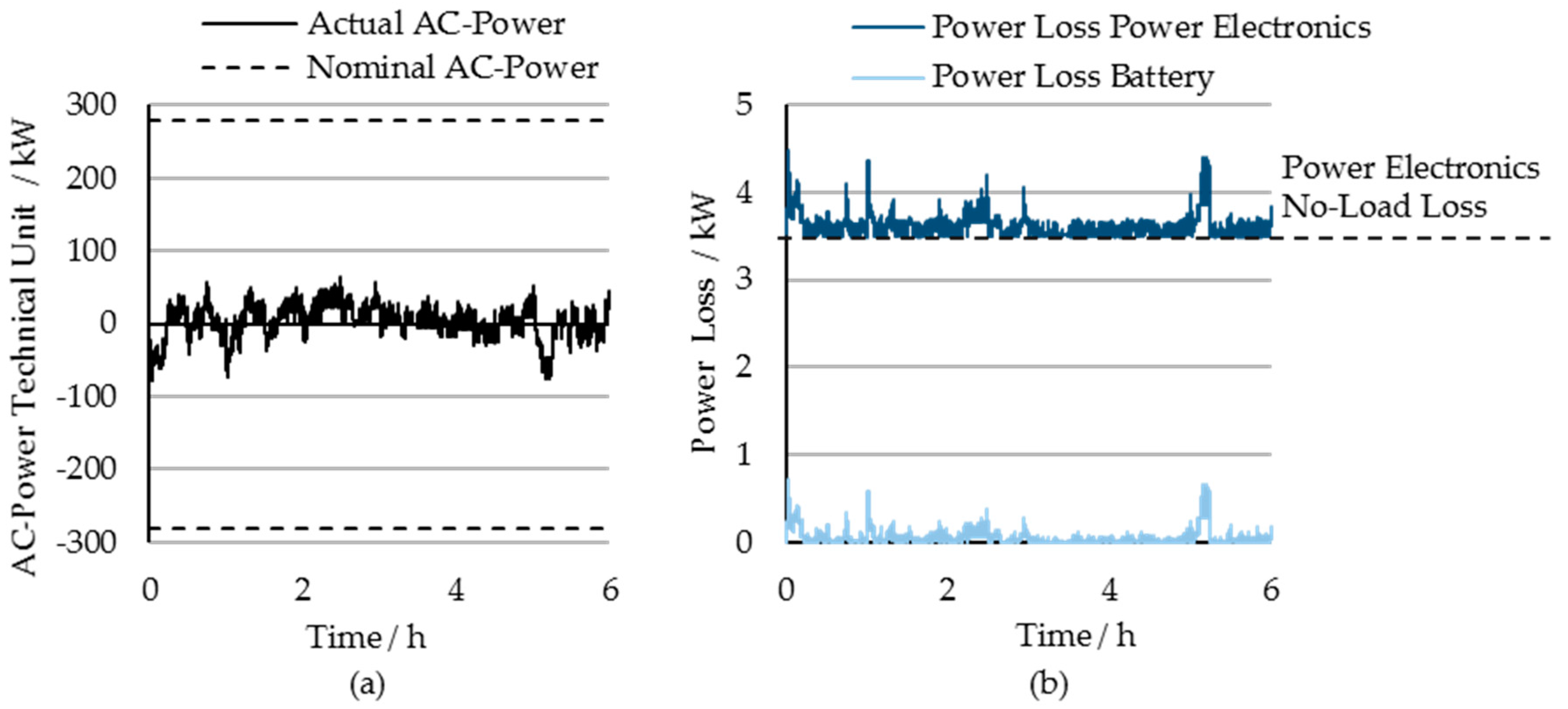
Figure 6a shows the measured AC-side power of TU 6 (
: Charge,
: Discharge) over time. Within the representative duration of six arbitrary hours, the maximum absolute power is 78.92 kW, and the average of the absolute power is only 16.52 kW. Both values are relatively small in comparison to the nominal PE power of 280 kW. The selected duration is representative of the available data in terms of two aspects: (I) grid frequency fluctuations constantly require the operation of the TU; and (II) TU power is on average low.
The resulting power losses (simulated data) are shown in
Figure 6b. The PE losses here constantly show a high offset value as the PE is in operation at all times. The offset value is also high in comparison to additional dynamic losses or to the battery losses, which confirms the previous findings of the TU loss analysis (see
Figure 5).
The conclusion from the loss analysis is that the PE no-load losses are the largest contributor to the system losses. As the losses can only be avoided when the PE unit is turned off, an analysis of the actual power demand is conducted to evaluate if this is an option considering the load profile.
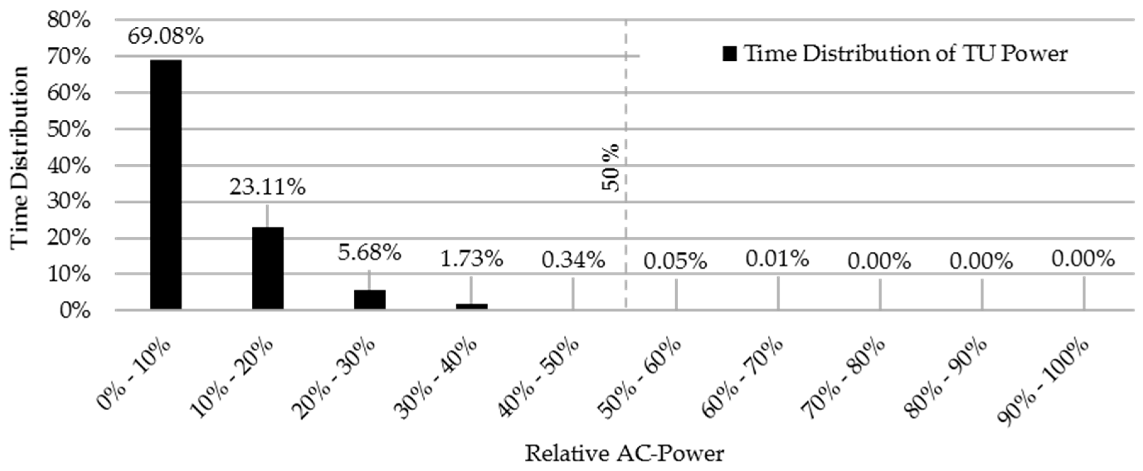
Figure 7 shows the temporal distribution of the relative power of TU 5 in March 2017.
Most of the time, the power is low: 99.95% of the time, the relative power is under 50%. As TU 3–5 consist of two power strings of identical setup, during this time, theoretically, only a single power string would be sufficient for providing the output power. This result motivates the development of an optimized PFDS that uses this optimization potential.

 ,
, 


