Optimization of a Coil System for Generating Uniform Magnetic Fields inside a Cubic Magnetic Shield

Abstract

Ultra-low magnetic fields have drawn lots of attention due to their important role in scientific and technological research. The combination of a magnetic shield and an active compensation coil is adopted in most high performance magnetically shielded rooms. Special consideration needs to be taken in the coil design since the magnetic shield significantly affects the uniformity of the magnetic field that is generated by the coil. An analytical model for the magnetic field calculation of the coil inside a cubic magnetic shield is proposed based on the generalized image method, which is validated by finite element analysis. A novel design method of the coil used in a cubic magnetic shield with a large homogeneous volume is proposed. The coil parameters are optimized to obtain a large cubic uniform volume with desired total deviation rate by discretizing the central volume in the coil. In the desired total deviation rate, the normalized usable volume of the new coil increases by 70% when compared with the Merritt coil. A coil system is developed according to the parameters obtained based on this method. The magnetic flux density and practical deviation rate of the coil are measured to validate the accuracy of this model and the feasibility of the design method. The experimental magnetic flux density agrees well with the analytical value. The maximum practical deviation rate of uniform volume of 0.8 × 0.8 × 0.8 m is in good agreement with the theoretical design value, taking into account the experiment errors.

1. Introduction

Ultra-low magnetic fields have important applications in the fields of particle physics, aerospace, magnetometry, geomagnetic navigation, and weak magnetism biology [1,2,3,4]. High performance magnetically shielded rooms (MSRs) are constructed to obtain ultra-low magnetic fields, which often adopt the combination of passive magnetic shielding and active magnetic shielding. The passive magnetic shield has been extensively used for high frequency ranges. To shield static and very low frequency magnetic fields, active compensation coils are widely used because of low costs when compared with the passive magnetic shield [5,6]. There are two main objectives for this combination in MSRs. One is to shield high frequency magnetic fields and the geomagnetic field. The combination reduces costs and improves the shielding performance. The other one is to obtain the desired uniform magnetic field inside the shield thanks to a dedicated coil. The magnetic shield, which is made of ferromagnetic material, causes a substantial reduction in the uniform volume of the coil, which needs to be considered when designing the coil [7,8,9,10,11].

The design of a coil inside a magnetic shield is generally limited to one of the following scenarios according to the shape of the shield. (1) The analytical model of the circular coil that is used inside a cylindrical magnetic shield is established for the coil design, whose premise is the cylindrical magnetic shield considered as an infinitely long shield [8,9,10]. Two pairs of solenoid coils that were designed for electric dipole moment (EDM) experiments at Tokyo Institute of Technology were used inside a cylindrical magnetic shield with a length to diameter ratio 1.7 [10]. A radial coil is proposed that produces highly uniform magnetic fields inside a cylindrical ferromagnetic shield [11]. (2) The currently best magnetically shielded rooms are the BMSR-II at Physikalisch Technische Bundesanstalt (PTB) in Berlin, using the square coils inside a cubic magnetic shield without a systematic design method [12].

Large magnetically shielded rooms cannot adopt cylindrical magnetic shield because of the limitation of manufacturer technology. The famous high performance MSRs such as the BMSR and BMSR-II of PTB, MSR of Athinoula A. Martinos Center in America, MSR of Technische Universität München in Germany, are all cubic magnetically shielded rooms [13,14]. In order to make full use of the space, the coils are placed so that they almost touch the inner surface of the shield, one has to take into account the coupling effect of the coil and the shield. For the design of the coil, it is necessary to establish an analytic model of coils inside the cubic shield to calculate the magnetic field. The analytical model of coils inside the cubic shield is different from that inside the cylindrical shield since the shield cannot be equivalent to an infinitely long shield. At present, there is no paper to propose a method of designing a coil inside a cubic shield.

The homogeneous volume of conventional coils is degraded when the coils used in a magnetic shield. This paper provides a novel design method of the coil used in a cubic magnetic shield with a large homogeneous volume. Firstly, the analytical model is established and verified by finite elements analysis. Secondly, a new design method of the coil used inside the cubic magnetic shield is put forward based on the analytical model in this paper. Finally, the performance of a coil system that is developed according to the new method is evaluated. It demonstrates the accuracy of the analytical model and the validity of the design method. The coil can be used for providing a large homogeneous volume for experiment in the MSRs. It can also be used for Earth field compensation and active shielding in high performance MSRs.

2. Influence of the Magnetic Shield

Coil systems are used to generate magnetic fields for physics and biology experiments, sensors calibration, and so on. Some conventional square coil designs are the square Helmholtz and Merritt coils. The square Helmholtz coil consists of two identical square coils that are placed symmetrically along a common axis. Two coils are separated by a distance of 0.5445 times the length of the coil. Each coil carries an equal electrical current flowing in the same direction. The Merritt coil consists of four identical square coils placed symmetrically along a common axis. The two outer coils have ∼2.361197 times the current to the inner coils. Inner coils are separated by ∼0.256212 times their length, whilst the outer coils are separated by ∼1.010984 times their length.

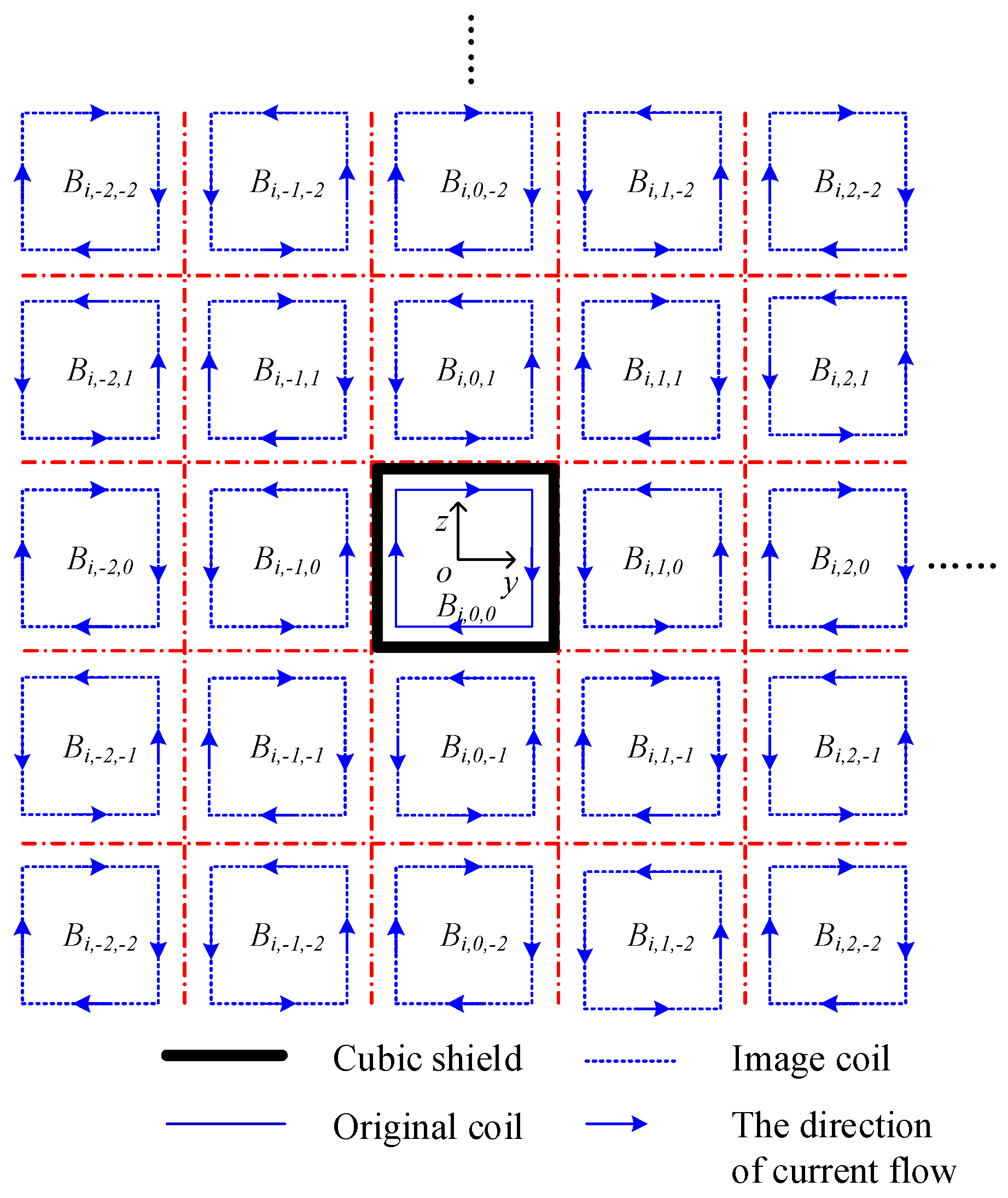
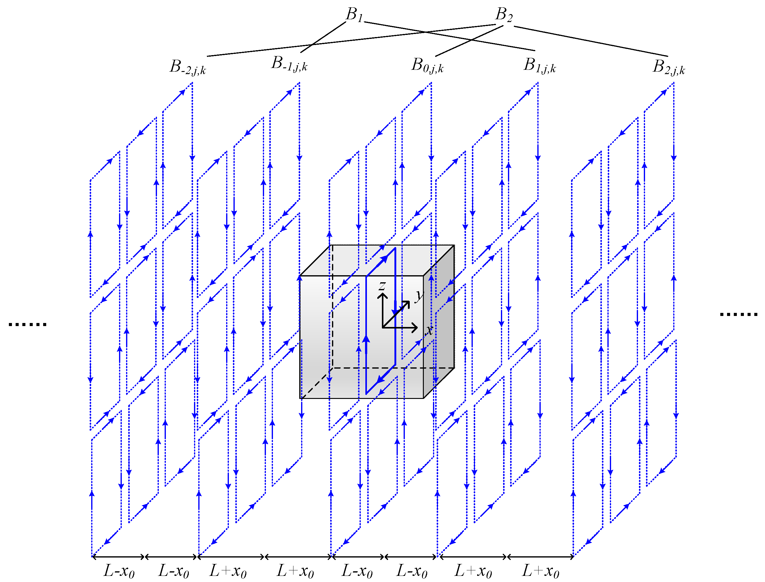
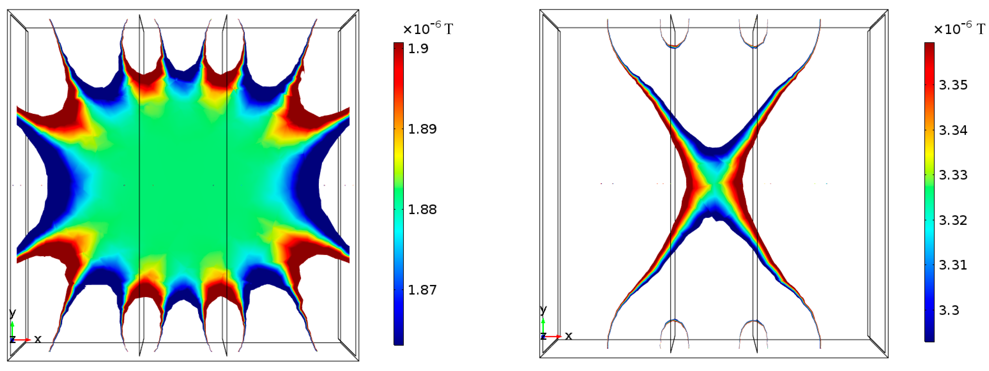
The magnetic field uniformity of the coil system used inside the magnetic shield is degraded by the magnetic shield. The magnetic shield imposes a ferromagnetic boundary condition that leads to a kind of mirror effect concerning the current loops [15]. It enhances the ability of the coil to generate large magnetic fields. In order to explore the effect of magnetic shield on the uniform volume that is generated by the coil, a one-axial Merritt coil is placed inside a cubic shield with 1.85 m side length [16,17]. The thickness of the shield layer is 1 cm and the relative permeability is 50,000. The axis of the coil is the x-axis. The center of the coil coincides with the center of the shield. Key parameters of Merritt coil are shown in

Table 1. Key parameters of Merritt coil.

Items	Value
Side length of the Merritt coil	1.8 m
Spacing of two inner coils	0.46 m
Spacing of two outer coils	1.82 m
Current value of two inner coils	0.85 A
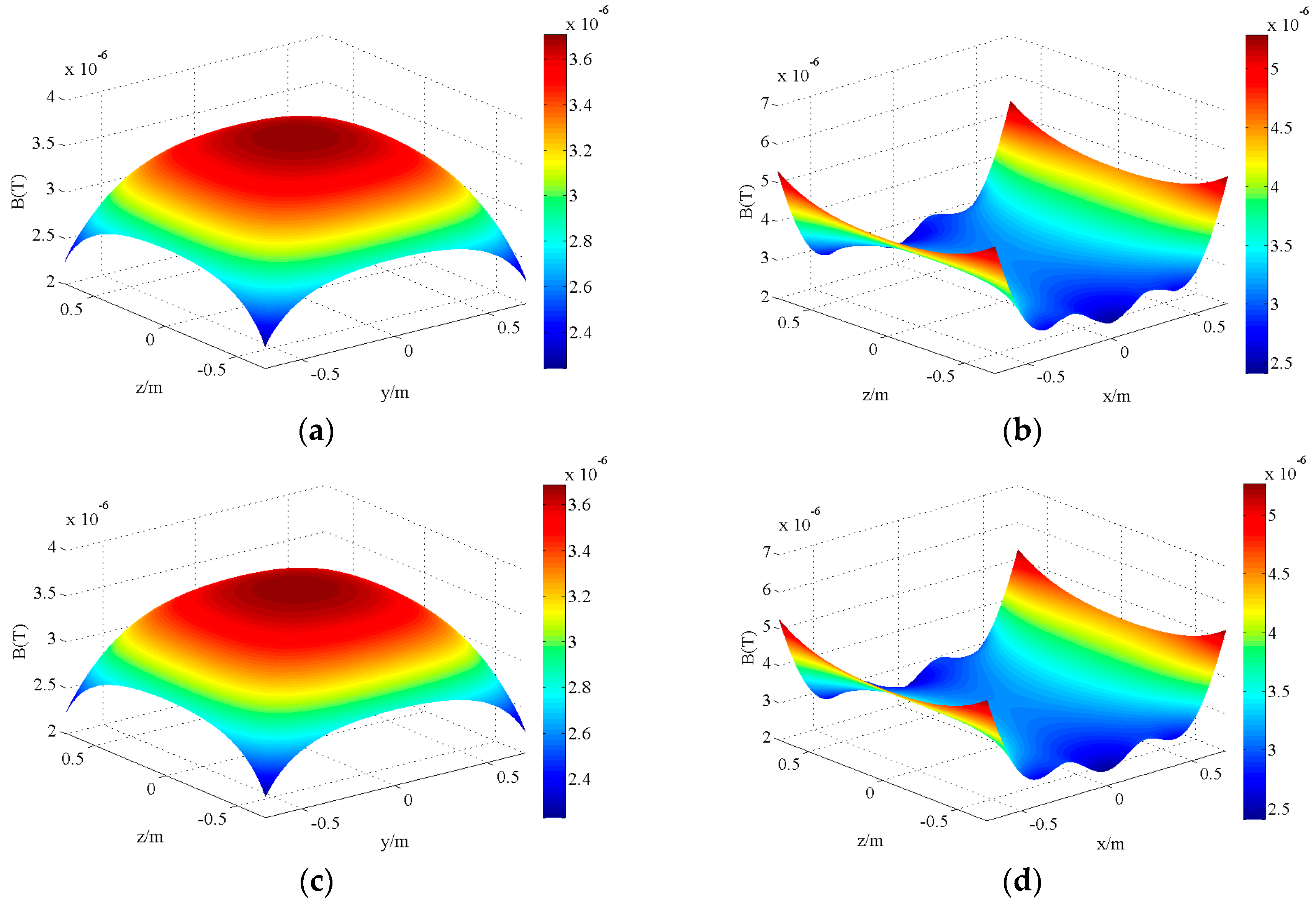
Current value of two outer coils	2 A

. The magnetic flux density that is generated by Merritt coil inside the cubic shield are simulated in COMSOL (COMSOL Multiphysics, Stockholm, Sweden), and compared with the flux density generated by Merritt coil without any shield, as shown in Figure 1. B^c is the flux density at the center, B(x, y, z) is the flux density at (x, y, z) point, the practical deviation rate of flux density between (x, y, z) and the center point is defined as Equation (1), which is a conventional index in practice [18].

$$\Delta B_{pr}=\frac{\left|B(x,y,z)-B^c\right|}{B^c}\times 100\%$$

(1)

It can be seen that the magnetic field uniformity generated by Merritt coil inside the cubic shield is very significantly degraded. Conventional coil systems, such as Merritt coil, Braunbeck coil, and square Helmholtz coil cannot be used directly in the cubic shield and a new coil needs to be designed to guarantee optimal performance inside the shield.

3. Analytical Model

3.1. Magnetic Field Calculation of Straight Line Segment

Designing the coil inside the cubic shield requires the establishment of an analytical model of magnetic fields. Firstly, the magnetic flux densities of a square coil are derived. A square coil consists of straight line segments current. The coil carries direct current generating static magnetic field. The flux density that is generated by the straight line segment current in space can be obtained thanks to the Biot-Savart law. The two ends of the straight line are a(x_a, y_a, z_a) and b(x_b, y_b, z_b). The magnetic flux density generated at any point p(x_p, y_p, z_p) is expressed as Equation (2), which contains three components. The total magnetic field at each point is obtained by considering the superposition law.

$$\begin{array}{l}{B}_x=\frac{\mu I}{4\pi }({\displaystyle {\int }_{y_a}^{y_b}\frac{(z_P-z)}{r^3}}dy-{\displaystyle {\int }_{z_a}^{z_b}\frac{(y_P-y)}{r^3}}dz)\\ B_y=\frac{\mu I}{4\pi }({\displaystyle {\int }_{z_a}^{z_b}\frac{(x_P-x)}{r^3}}dz-{\displaystyle {\int }_{x_a}^{x_b}\frac{(z_P-z)}{r^3}}dx)\\ B_z=\frac{\mu I}{4\pi }({\displaystyle {\int }_{x_a}^{x_b}\frac{(y_P-y)}{r^3}}dx-{\displaystyle {\int }_{y_a}^{y_b}\frac{(x_P-x)}{r^3}}dy)\end{array}$$

(2)

3.2. Analytical Model Based on the Generalized Image Method

An analytical model of a square coil inside the cubic shield is established based on the generalized image method. The center of the shield coincides with the center of the coil. Side length of the shield is 2L, side length of the coil is 2l. The shield has six planes, namely, two parallel xy planes, two parallel yz planes, and two parallel xz planes. In ambient geomagnetic field conditions, permalloy material is not saturated, so the thickness of the permalloy is of no concern for our problem.

3.2.1. Image Coils Created for Boundary Conditions in xy Planes and xz Planes

When two xy planes and two xz planes are considered, as shown in Figure 2, the images have periodicities of 2L in the y-direction and z-direction [19]. The image coils and the original coil have the same current value. The direction of current flow and position of the image coils follow the law of the image method as shown in Figure 2. The original coil is centered at (x₀, 0, 0) point, f_i,j,k(x_i, y_j, z_k) represents the flux density generated by the coil centered at (x_i, y_j, z_k) point, i, j, and k are the subscript for numbering in the x-, y- and z-directions. The flux density of the original coil can be expressed as

$$\begin{array}{l}{f}_{{}_{0,0,0}}(x_0,0,0)=B(a,b)+B(b,c)+B(c,d)+B(d,a)\\ \left(\begin{array}{cccc}a(x_0,l,l);& b(x_0,-l,l);& c(x_0,-l,-l);& d(x_0,l,-l)\end{array}\right)\end{array}$$

(3)

Here, for example, B(a, b) is calculated by Equation (2), which represents the magnetic field intensity of the straight current with a and b as the end points. The flux density that is generated by the original and image coils at plane x = x₀ can be expressed as

$$\begin{array}{l}{B}_{i,j,k}={\displaystyle \sum _j{\displaystyle \sum _k{f}_{{}_{0,j,k}}}}(x_0,2jL,2kL)\\ \left(\begin{array}{ccc}i=0;& j=0,\pm 1,\pm 2,\cdots ;& k=0,\pm 1,\pm 2,\cdots \end{array}\right)\end{array}$$

(4)

3.2.2. Image Coils Created for Boundary Conditions in xy, xz and yz Planes

When xy, xz, and yz planes are considered, the two-dimensional (2-D) pattern of the original coil and image coils will be extended into 3-D pattern, as shown in Figure 3. The image distribution is periodic in the x-, y-, and z-directions. There are an infinite number of image coils. The image coils can be divided into two groups to calculate according to their x coordinates, such as Equations (5) and (6). The flux density of the combined effect of the original coil and the boundary conditions on all the six planes can be expressed as Equation (7).

$$\begin{array}{l}{B}_1={\displaystyle \sum _i{\displaystyle \sum _j{\displaystyle \sum _k{f}_{{}_{i,j,k}}(2L-x_0+4iL,2jL,2kL)}}}\\ \left(\begin{array}{ccc}i=\pm 1,\pm 3,\cdots ;& j=0,\pm 1,\pm 2,\cdots ;& k=0,\pm 1,\pm 2,\cdots \end{array}\right)\end{array}$$

(5)

$$\begin{array}{l}{B}_2={\displaystyle \sum _i{\displaystyle \sum _j{\displaystyle \sum _k{f}_{{}_{i,j,k}}(x_0+4iL,2jL,2kL)}}}\\ \left(\begin{array}{ccc}i=0,\pm 2,\pm 4,\cdots ;& j=0,\pm 1,\pm 2,\cdots ;& k=0,\pm 1,\pm 2,\cdots \end{array}\right)\end{array}$$

(6)

$$B=B_1+B_2$$

(7)

3.3. Verification by Finite Element Analysis

The analytical model is verified by the finite element method (FEM) by using COMSOL. The finite elements simulations of the flux density generated by a Merritt coil inside the cubic shield were compared with the analytical solutions that were computed in Matlab. Parameters of the Merritt coil and the cubic shield are the same as previously mentioned. A model of the coil inside the shield was built in COMSOL. The boundary condition is set that the thickness of the magnetic shield is 1 cm with the relative permeability of 50,000. The mesh type of the model is tetrahedron mesh and the model is divided into 1,775,865 elements. The flux density of the coil has the same distribution in the y- and z-directions because of the coil symmetrical structure, so that just show the flux density distribution of planes perpendicular to x and y axes. Figure 4a shows that there is an approximately uniform flux density area around the center and the flux density away from the center gradually decreases. Figure 4b shows that the distribution of the flux density is saddle-shaped. Figure 4c,d show that the FEM results are in good agreement with the analytical results.

The relative errors between the analytical and the finite elements calculations of the generated flux density in several planes are shown in Figure 5. The relative error of less than 0.83% between the analytical value and the finite elements analysis value demonstrates the accuracy of the model. Due to the limited computational ability of the computer, there is a certain error of the model that is simulated in COMSOL. This is one of the sources of the relative error between analytical and finite element results.

4. Coil Design

Tri-axial coil systems widely used in MSR are a combination of well-designed one-axial coils. Therefore, the design of a coil will refer to the mono axial coil. There are two main criteria of a coil, the flux density deviation rate, and its corresponding uniform volume. Take the excitation of the x-axis coil for example: B^c is the magnetic flux density at the center which only has x component. The change in the magnetic flux density away from center is normalized relative to B^c. For a perfect field uniformity within the volume of the coil system, $B_y=B_z=0$ and $B_x=B_x^c$, this definition is equivalent to the definition of the flux density that is uniformity presented in Equation (8), the total deviation rate ΔB_T is defined as Equation (9) [20,21]. For a given magnetic field deviation, the larger the uniform volume of the coil system, the better for the application. However, a slender uniform area has a low utilization in most cases. So, we define uniform volume V_m, which is the maximum cubic volume that the uniform area can accommodate in a certain deviation.

$$\begin{array}{l}\Delta B_x(\%)=100\left|(\left|B_x\right|-\left|B_x^c\right|)/B_x^c\right|\\ \Delta B_y(\%)=100\left|B_y/B_x^c\right|\\ \Delta B_z(\%)=100\left|B_z/B_x^c\right|\end{array}$$

(8)

$$\Delta B_T(\%)=\sqrt{\Delta B_x^2+\Delta B_y^2+\Delta B_z^2}=100\sqrt{\left[{(\left|B_x\right|-\left|B_x^c\right|)}^2+{\left|B_y\right|}^2+{\left|B_z\right|}^2\right]/{\left|B_x^c\right|}^2}$$

(9)

The more coils per axis, the higher uniformity and larger uniform region achievable. However, since the alignment of many coils is difficult, large coil systems mostly use four coils for one axis [22]. So, we adopt the design of a four-coil system for one axis. The new coil consists of four identical square coils, which is similar to Merritt coil.

Setting the length of coils as l and the current value of the two inner coils as I₂, and when considering that the four coils have the same number of turns, the coil system can be described thanks to three variables: the spacing between the two outer coils 2a, the spacing between the two inner coils 2b, and the current of the two outer coils I₁.

The optimization of the coil used inside the cubic magnetic shield consists in finding the optimal value of the three variables so that the coil has the largest uniform area V_m in for a given deviation. The common deviation rate is 1% in application, we set a slightly higher theoretical target of 0.85% when considering the performance of practical coils will be worse. So, we focused on the uniform volume of 0.85% deviation rate. A cubic computational volume V is defined inside the coil whose center coincides with the center of the coil, which is the green volume in Figure 6. We discretize the volume V and divide it into n × n × n grid points. If ΔB_T of all the points in the volume is less than 0.85%, U equals one which means the total deviation rate of the region is less than 0.85%.

$$U=\frac{\mathrm{Number}\mathrm{of}\mathrm{points}\mathrm{which}\mathrm{satisfy}\Delta B_T<0.85\%}{\mathrm{Total}\mathrm{number}\mathrm{of}\mathrm{points}{n}^3}$$

(10)

The flow chart of the coil design method is shown in Figure 7. Firstly, the values of parameters V, l, I₂, and the ranges of three variables 2b, 2a, I₁ are chosen. Parameters of several sets of the coil are then generated according to the ranges of variables. Calculate U of the volume V, if more than one set of coils meet the condition that U equal to 1, expand the volume V, and repeat the above calculation until only one set of the coil meet the condition.

Practically, the side length of the magnetically shielded room is 1.85 m. Because of the space constraint, the largest side length of the coil that can be assembled in the room is 1.55 m. The values of parameters and the range of variables are given in

Table 2. The values parameters and the range of variables.

Symbols	Items	Value
V	Initial computational volume	0.1 × 0.1 × 0.1 m
l	Side length of coil	1.55 m
I2	Current value of the two inner coils	8 A
I1	Current value of the two outer coils	[0, 3I2]
2b	Spacing of the two inner coils	[0, 0.5l]
2a	Spacing of the two outer coils	[[0.5l, 1l]

.

With the small cubic computational volume, U takes the maximum value 1 for several, parameters corresponding to different coil designs are obtained. The volume is then progressively extended outwards, until only one coil design satisfies the homogeneity criterion. The uniform volume V_m of the new coil is 0.8 × 0.8 × 0.8 m. Key parameters of the coil have been tabulated in

Table 3. Key parameters of the coil.

l	I2	2b	2a	I1
1.55 m	8 A	0.258l	0.839l	1.25I2

.

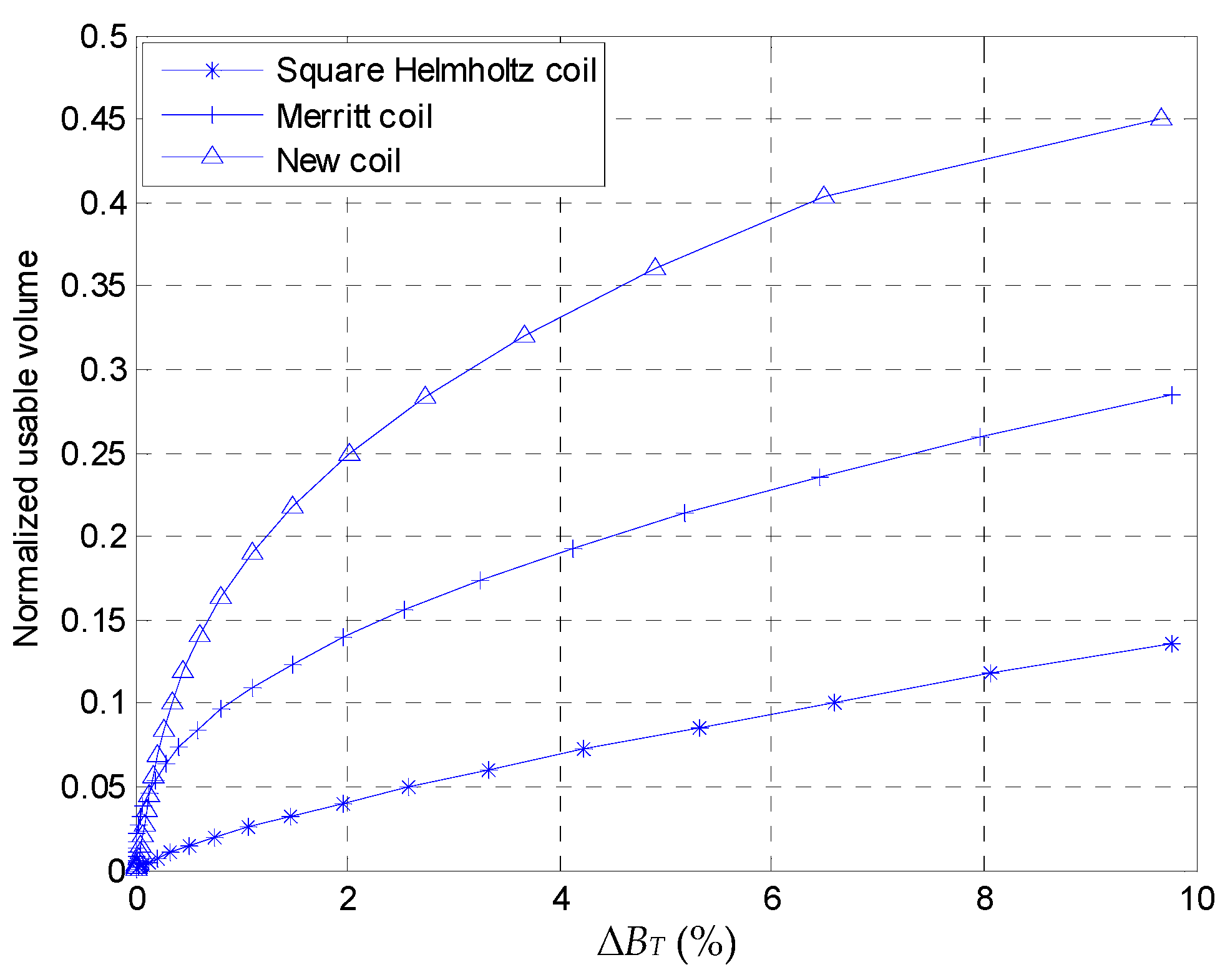
In order to compare the effectiveness of different coils, the ratios of the uniform volume to the total volume bounded by the coil (referred to as the normalized usable volume) are shown in Figure 8 for classical structures (Square Helmholtz and Merritt coils) and our proposed design.

Figure 8 shows that the Merritt coil and the new coil have larger normalized usable volumes than the square Helmholtz coil. It can be explained by the fact that they consist of more coils per axis resulting in an increased ability to produce a uniform volume. Both the Merritt coil and the new coil consist of four identical coils per axis. But, the new coil that is used in the shield provides a larger normalized usable volume than the Merritt coil. The reason is that the design method enhances the ability of the new coil to produce a large homogeneous volume. Besides, the design narrows distance between the outer two coils, thus the total volume of the coil is reduced. It also increases the normalized usable volume of the new coil. In the desired total deviation rate 0.85%, the normalized usable volume increases by 70% for the new coil relatively to the Merritt coil.

5. Experiment

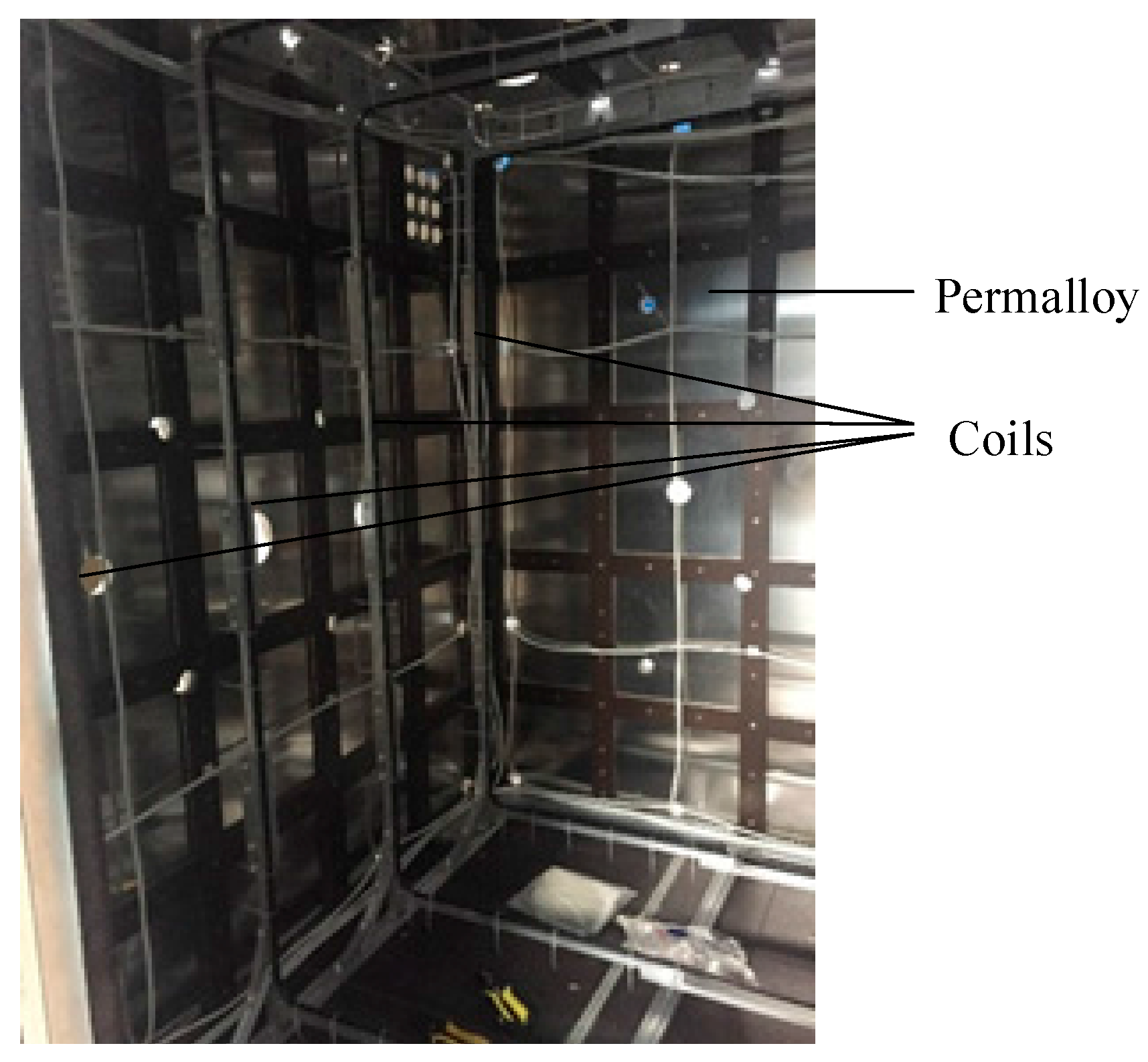
The aim of the experiment is to measure the magnetic field uniformity of 0.8 × 0.8 × 0.8 m size generated by the new coil system inside a magnetically shielded room to verify our model predictions. The MSR in Harbin Institute of Technology is a cubic magnetic shield with the 1.85 m side length. The MSR consists of one permalloy layer of 2 mm thickness.

The key to the development of the coil system is the selection of materials of the frame and the coil, and the calculation of the wire diameter. Since magnetic materials might distort the magnetic field, the frame and fastenings are made of non-magnetic aluminum alloy, bolts, and nuts are made of nylon. Cables are attached to the frame to make square coils. A prototype of the new coil system is illustrated in Figure 9. The cables consist of five 1 mm² section wires.

The coil performance test system consists of a constant current source, a magnetic field sensor, and a sensor stand. We use a three-axis magnetic field sensor Mag-03 of Bartington Company for measuring. The sensor is fixed on the stand that is also made of aluminum alloy and is movable and height adjustable. The sensor is moved to the center of the coil to measure the flux density firstly. Given the coil system and the MSR symmetry, flux density was measured within a volume of 0.4(−0.4 m $\le$ x $\le$ 0 m) × 0.4(−0.4 m $\le$ y $\le$ 0 m) × 0.4(0 m $\le$ z $\le$ 0.4 m) instead of the whole volume of the coil for the sake of experimental efficiency. Magnetic flux density is measured at grid points located every 10 cm along the x, y and z directions.

6. Results

The FEM, analytical, and experimental results at the center of the coil are compared in

Table 4. Magnetic flux density of the coil at the center.

Items	Bx (µT)	By (μT)	Bz (μT)	B (μT)
FEM	24.527	0	0	24.527
Analytical	24.508	0	0	24.508
Experimental	24.505	0.073	0.53	24.511

. It can be seen from the table that there is no y, z component of the magnetic flux density of the center point in theory. However, the experimental value have y, z component since we cannot make sure that the x, y, and z axes of the coil system coincide strictly with the x, y, and z axes of the sensor. In the uniform volume, x component of the flux density is large, and the y and z components are almost zero in theory. Due to the large x component of the flux density, the slight deviation of the sensor’s coordinate axes result in a large error in measuring the y and z components of the flux density. 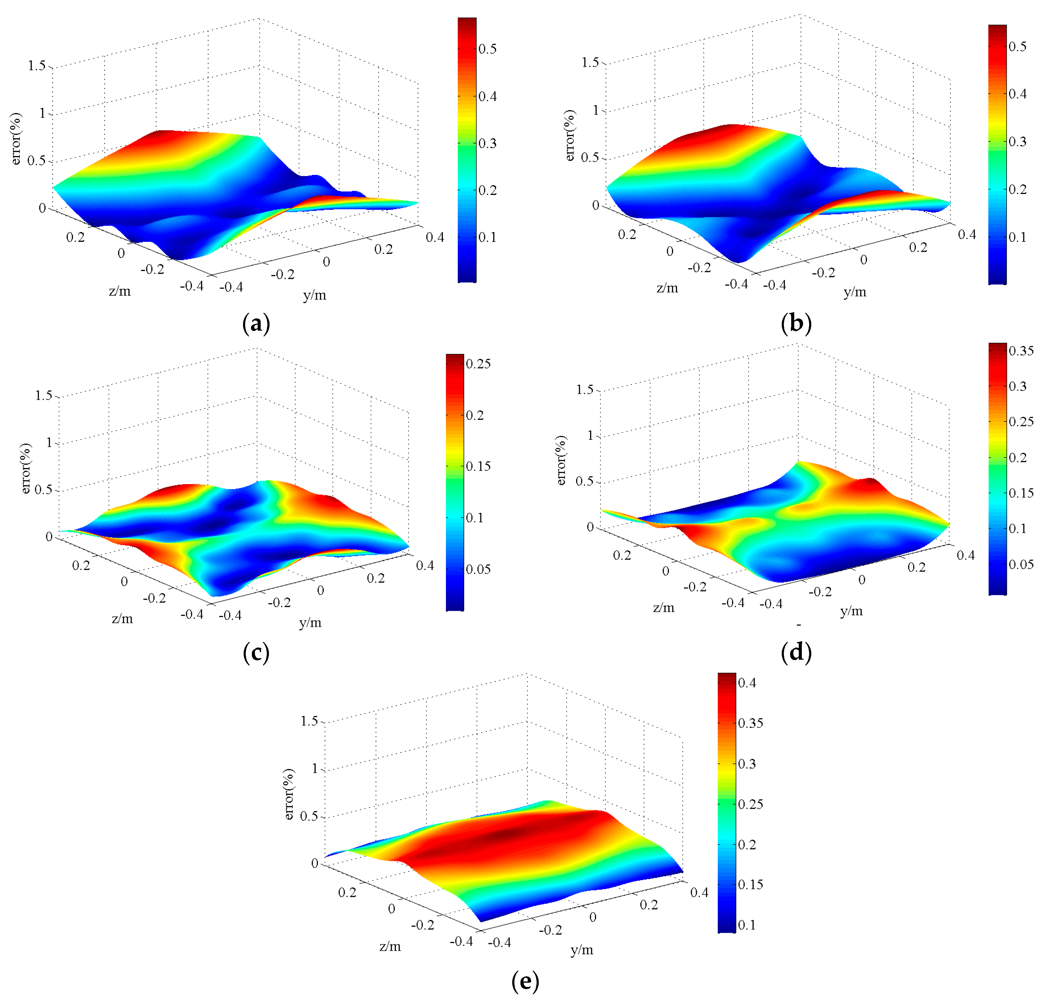So, we just focus on the x component of the flux density and flux density amplitude. Values of the measuring points are fitted and the relative errors between the analytical and experimental results are calculated, as shown in Figure 10 and Figure 11. There are small relative errors of below 0.566% between the analytical and experimental x component of the flux density and 0.570% between the analytical and experimental flux density amplitude.

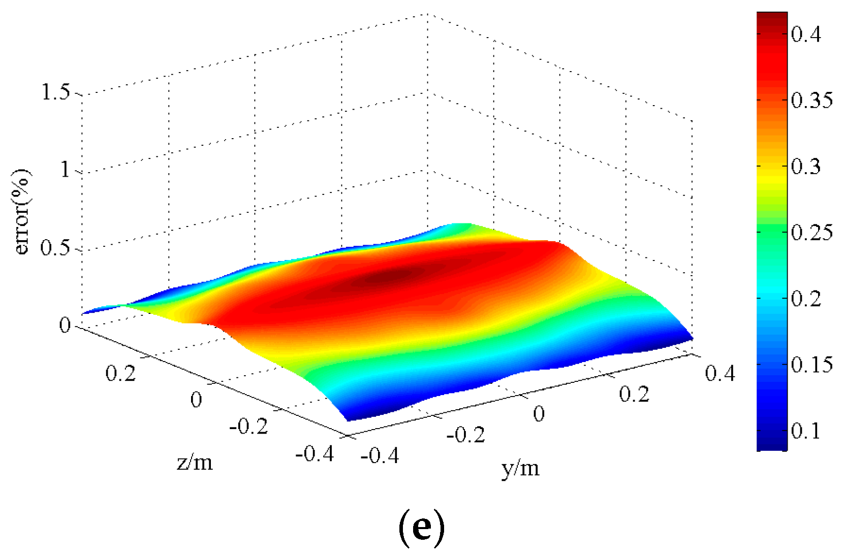
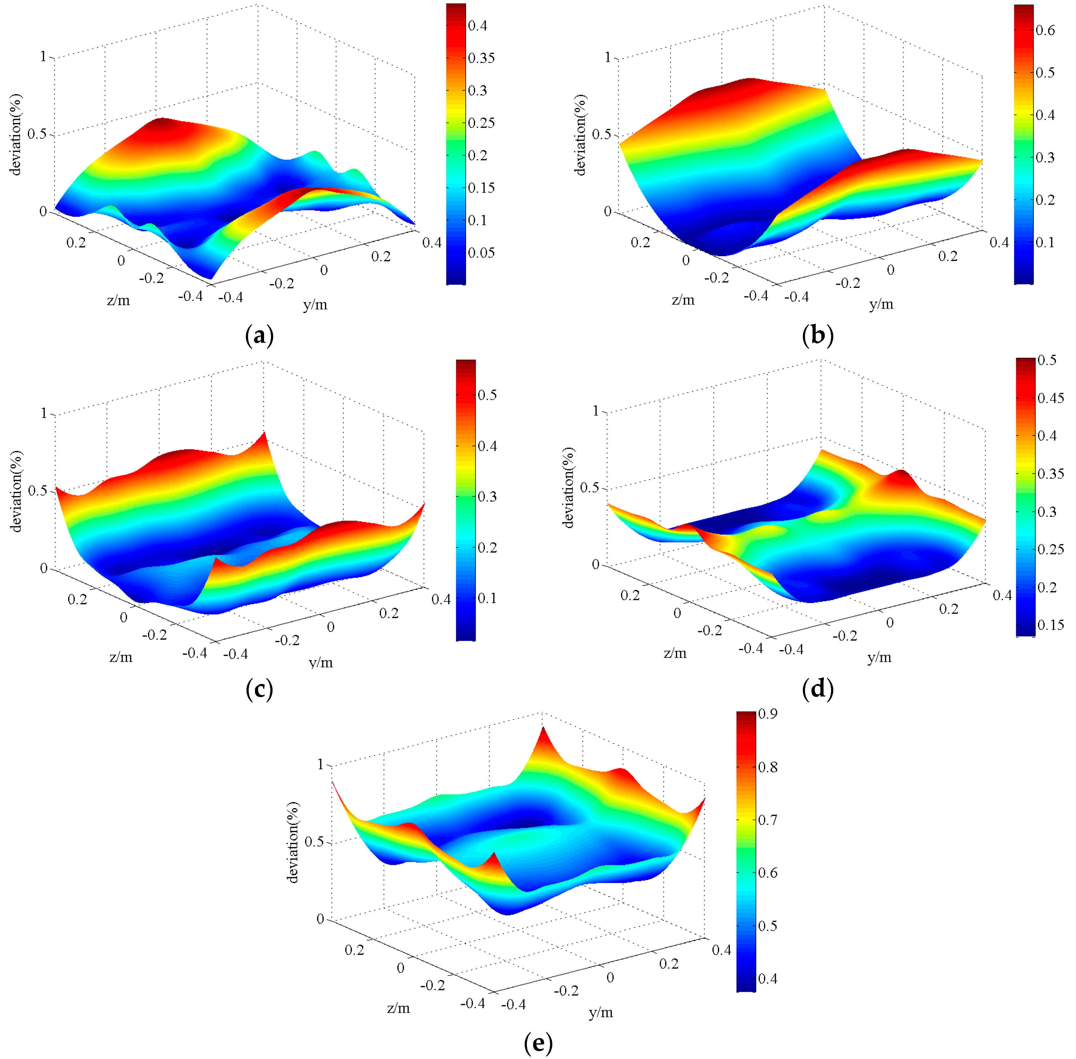
There are some reasons for relative errors. (1) The MSR is an ideal cubic layer in the analytical model. The actual MSR is made of pieces of permalloy plate. The room has a door and a number of holes for ventilation. (2) The coils deformation and alignment mismatch can cause the errors. Since there may be a little deviation between the axes of the coil and axes of the sensor, we use practical deviation rate ΔB_pr as the index that only contains the amplitude of flux density. The practical deviation rates of the measuring points are calculated and fitted, as shown in Figure 12. The maximum value of the practical deviation rates of the measuring points is 0.920%, which is in good agreement with the theoretical value 0.804%.

7. Conclusions

The aim of this paper is to propose a novel design method of the coil that is used inside a cubic magnetic shield with a large homogeneous volume. An analytical model for magnetic fields calculation of coils inside the cubic magnetic shield is established. The validity of the analytical model is verified by the finite elements analysis and experiments. Based on the analytical model, a new coil system is put forward by using the design method. In the desired total deviation rate, the normalized usable volume of the new coil increases by 70% when compared to the Merritt coil. The magnetic flux density and the practical deviation rate of the new coil are measured, which are in good agreement with the analytical results.

The new coil has a smaller spacing of two outer coils and current ratio of outer coils to the inner coils than the Merritt coil. The geometrical configuration of the new coil is adapted to the cubic magnetic shield since the shield enhances the ability of the coil to generate magnetic fields. The new coil design has a distinct advantage over conventional coil designs because it can provide a large homogeneous volume in the cubic magnetic shield. Harbin Institute of Technology is planning to build a high performance magnetically shielded room. This is a basic research for designing an active compensation coil of the geomagnetic field shielding and a coil with a large homogeneous volume for experiment in the MSR.